| Issue |
A&A
Volume 664, August 2022
|
|
|---|---|---|
| Article Number | A101 | |
| Number of page(s) | 9 | |
| Section | Stellar structure and evolution | |
| DOI | https://doi.org/10.1051/0004-6361/202243573 | |
| Published online | 10 August 2022 | |
Exploratory scenarios for the differential nuclear and tidal evolution of TZ Fornacis
1
Instituto de Astrofísica de Andalucía, CSIC, Apartado 3004, 18080 Granada, Spain
e-mail: This email address is being protected from spambots. You need JavaScript enabled to view it.
2
Dept. Física Teórica y del Cosmos, Universidad de Granada, Campus de Fuentenueva s/n, 10871 Granada, Spain
Received:
17
March
2022
Accepted:
6
June
2022
Abstract
Aims. TZ Fornacis is a double-lined eclipsing binary system with similar masses (2.057 ± 0.001 and 1.958 ± 0.001 M⊙) but characterized by very different radii (8.28 ± 0.22 and 3.94 ± 0.17 R⊙). This similarity in terms of mass makes it possible to study the system’s differential stellar evolution as well as some aspects of its tidal evolution. With regard to its orbital elements, it was recently confirmed that its orbit is circular with an orbital period of 75.7 days. The less massive component rotates about 17 times faster than the primary one, which is synchronized with the mean orbital angular velocity. Our main objective in this work is to study both the nuclear and the tidal evolution of the system.
Methods. To model the TZ For system, we used the MESA package, computing the grids using the exact observed masses, radii, and effective temperatures as input, and then varying the metallicity, the core overshooting amount, and the mixing-length parameter. A χ2 statistic was used to infer the optimal values of the core overshooting and the mixing-length parameters. The same procedure was used to generate rotating models with the GRANADA code. The respective errors in the average age of TZ For were less than 5%. On the other hand, the differential equations that govern the tidal evolution were integrated using the fifth-order Runge–Kutta method, ith a tolerance of 1 × 10⁻⁷.
Results. We explored two scenarios regarding the initial eccentricities: a high one (0.30) and a case of an initial circular orbit. A good agreement has been found between the observational values of the eccentricity, synchronism levels, and orbital period with the values predicted by the integration of the tidal evolution equations. The influence of the friction timescale on the evolution of the orbital elements of TZ For is also studied here. The orbital elements most affected by the uncertainties in the friction timescale are the synchronism levels of the two components. On the other hand, we used the properties of the rotating models generated by the GRANADA code as the initial angular velocities instead of using trial values. In this case, comparisons between the theoretical values of the orbital elements and their observed counterparts also lead to a good interagreement.
Key words: binaries: eclipsing / binaries: general / stars: evolution / stars: interiors / stars: fundamental parameters / stars: rotation
© A. Claret 2022
 Open Access article, published by EDP Sciences, under the terms of the Creative Commons Attribution License (https://creativecommons.org/licenses/by/4.0), which permits unrestricted use, distribution, and reproduction in any medium, provided the original work is properly cited.
This article is published in open access under the Subscribe-to-Open model. This email address is being protected from spambots. You need JavaScript enabled to view it. to support open access publication.
1. Introduction
TZ Fornacis (TZ For) is a very evolved double-lined eclipsing binary (DLEBS) that was first accurately investigated by Andersen et al. (1991); see also Torres et al. (2010). Furthermore, TZ Gallenne et al. (2016) revised the absolute dimensions of this system using interferometric observations combined with new radial velocity measurements and confirmed that the system demonstrates very similar components in mass (2.057 ± 0.001 and 1.958 ± 0.001 M⊙), but with very different radii: 8.28 ± 0.22 and 3.94 ± 0.17 R⊙, respectively. The effective temperatures for both components are 4930 ± 30 K and 6650 ± 200 K and the orbital period is ≈75.7 days. This mass similarity and the accuracy of the absolute dimensions makes TZ For a good laboratory for the study of its differential stellar evolution as well as some aspects of its tidal evolution. In fact, both components evolve quite similarly in the main sequence, however, during the very fast phases of their evolution, we can significant changes in the effective temperatures and also in their radii, apsidal motion constants, and moment of inertia – on the basis of stellar evolutionary models. Concerning its tidal evolution, Andersen et al. (1991) established a circular orbit for TZ For and these authors also found that while the primary rotates synchronously with the mean orbital angular velocity, the secondary rotates approximately 16 times faster than its respective value of synchronisation, which is on the order of 2.6 ± 0.1 km s−1. These results are consistent with those obtained by Gallenne et al. (2016).
One of the first attempts to explain some aspects of both nuclear and tidal evolution was carried out by Claret & Giménez (1995), who adopted the hydrodynamical mechanism proposed by Tassoul (1987). However, that study did not provide a clear scenario of the stellar and dynamic evolution of the system since, at that time, the current position of the system in the HR diagram was not yet fully clear. Second, timescales for the circularisation and synchronisation were used (assuming a constant orbital period) instead of formally integrating the differential equations that govern the behavior of angular velocities, orbital period, and eccentricity. In addition, Rieutord (1992) presented some criticism on the hydrodynamical mechanism introduced by Tassoul (1987) regarding the inefficiency in reducing the synchronization time of the large-scale flows driven by Ekman pumping in the spin-up and down of a tidally distorted star. Later on, Tassoul & Tassoul (1996) refuted this argument. For a more extensive discussion on this subject, we refer to Rieutord (1992), Tassoul & Tassoul (1996), Claret & Cunha (1997). In fact, Claret & Cunha (1997) found some disagreements between the tidal evolution theories predictions and the observational values: while the hydrodynamic mechanism was indeed shown to be too efficient in circularizing the orbits, the opposite happened with the tidal torque process.
A number of years later, Claret (2011) tried a new approach to the problem. Instead of adopting the timescales as in Claret & Giménez (1995), which are valid only for low eccentricities and small departures from the synchronism, a more rigorous treatment was carried out. These authors found that while the first approximation can be considered roughly acceptable at least for the present status of TZ For (but not necessarily in the past), the second is not satisfied given the observed level of asynchronism of the secondary. To further improve on the previous method, the differential equations that govern the tidal evolution (eccentricity, angular velocities, and orbital period) were explicitly integrated adopting appropriate models computed with the GRANADA code (Claret 2004). Another point that was clarified in the 2011 paper was the position of the primary, which was located on the clump during the helium-burning phase.
In this paper, we propose a revision to the nuclear and dynamic evolution of the system by taking into account the most recent determinations of the absolute dimensions by Gallenne et al. (2016). Here, the expression nuclear evolution refers to the changes in effective temperatures, radii, luminosities, moments of inertia, and other effects caused by nuclear reactions in the stellar interior. To model the TZ For system, we computed stellar evolutionary tracks with the MESA Package, adopting the methodologies described in detail by Claret & Torres (2016, 2017, 2018, 2019). In addition, an updated version of the GRANADA code was used to simulate stellar rotation based on the assumption of a solid body configuration.
The paper is structured as follows. In Sect. 2, we briefly describe the stellar evolution code MESA and our methodology for deriving, for each star, the semi-empirical value of fov (overshooting parameter, see below) by comparing the observed absolute dimensions with a series of grids of stellar models for both components of TZ For. In this section, we also introduce the differential equations of tidal evolution. In Sect. 3, we analyse the stellar and tidal evolution for TZ For and summarise our results. Finally, in Appendix A, we describe the method for generating rotating models introduced by Kippenhahn & Thomas (1970) and implemented in the GRANADA code and adapted to the particular case of TZ For.
2. Stellar models and the differential equations of tidal evolution
2.1. Stellar models
The stellar evolutionary tracks used to fit the absolute dimensions of TZ For were computed using the Modules for Experiments in Stellar Astrophysics package (MESA; Paxton et al. 2011, 2013, 2015) version 7385. Microscopic diffusion was included and mass loss was considered following the formulation by Reimers (1977), with an efficiency coefficient of η = 0.2 (not to be confused with η of the Radau equation). For the convective envelopes, we employed the mixing-length formalism (Böhm-Vitense 1958), where αMLT is a free parameter. The calibrated value of the mixing-length parameter for the Sun in these models is αMLT = 1.84 for Z⊙ = 0.0134. For the opacities, we adopted the mixture given by Asplund et al. (2009). The enrichment law used in pairings with such opacities was ΔY/ΔZ = 1.67, with the primordial helium Yp = 0.249 following Ade et al. (2016). Convective core overshooting was considered in the diffusive approximation which is characterized by the free parameter fov. For more details, we refer to Freytag et al. (1996) and Herwig et al. (1997). The grids were computed starting from the pre-main sequence (PMS) and the effects of rotation were ignored for this set of models.
As previously commented, a series of papers by Claret & Torres (2016, 2017, 2018, 2019) used stellar evolutionary models and a select sample of 50 well-measured detached DLEBS to calibrate the dependency of core overshooting on stellar mass. Here, we use the results of one of these papers (Claret & Torres 2018) as a reference where the case of TZ For had already been analysed. In that paper, several grids were computed for this system using as a main input the exact observed masses, radii, and effective temperatures varying the metallicity, as well as the core overshooting amount and the mixing-length parameter. In the search for the best solution for the two components, we adopt a χ2 statistic to infer the optimal values of the overshooting and the mixing-length parameters. Due to intrinsic limitations in the stellar models (opacities, equations of state, mass loss, etc.) and considering the observational errors, the derived ages for the two components were allowed to differ by up to 5%. The best fits for TZ For, adopting the mixture by Asplund et al. (2009) and the enrichment law described above, are as follows: αMLT1 = 1.91, αMLT2 = 1.85 and fov1 = 0.017, and fov2 = 0.015 for a metallicity of Z = 0.015. The derived mean age of the two components is 1.13 ± 0.04 Gyr. Figure 1 shows the resulting HR diagram where the primary is located at the clump. We note that our solution is slightly different from that found by Gallenne et al. (2016) since these authors located the secondary near the red hook. Another interesting aspect derived from Claret & Torres (2018) is that if a different enrichment law is adopted for TZ For, for instance, ΔY/ΔZ = 1.0, we obtain essentially the same result: the primary is also in the core helium-burning phase (clump) and the secondary on the subgiant branch. This suggests that the fov parameter is insensitive to helium content for this particular case.
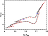 |
Fig. 1. HR diagram for TZ For. The models were calculated adopting Z = 0.015. Solid line indicates the primary component while the dashed one represents the secondary. |
On the other hand, TZ For was also recently studied by Costa et al. (2019), who used a different method from that of Claret & Torres (2017). The basic difference between the two methods is that Costa et al. (2019) introduced rotation into their models (taking into account rotational mixing) by assuming constant values of core overshooting and MLT parameters. According to these authors, they found: a good agreement with models computed with fixed overshooting parameter, λov = 0.4, and initial rotational rates, ω, uniformly distributed a in a wide range between 0 and 0.8 times the break-up value, at varying initial mass. We also note that their definition of λov is different from the one we used (diffusive approximation, characterized by the parameter fov).
2.2. Differential equations of tidal evolution
Here, we adopt the differential equations for the tidal evolution in the frame of the weak friction model (Hut 1981). The respective equations for an initial eccentricity different from zero can be written as:
 (1)
(1)
 (2)
(2)
 (3)
(3)
 (4)
(4)
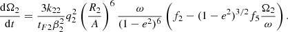
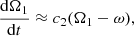
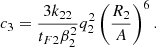
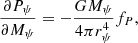
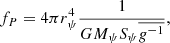
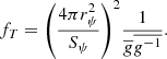
In the above equations, e is the orbital eccentricity, A is the semimajor axis, Ωi is the angular velocity of the component i, and ω is the mean orbital angular velocity, while βi is the radius of gyration of the component i, then k2i is the apsidal motion constant of the component i and Ri is the radius of the component i, and q = M2/M1, q2 = M1/M2 and tF is an estimation of the timescale of tidal friction which is given by:
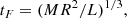 (5)
(5)
where L is the luminosity, R the radius, and M the stellar mass. For a solar-type star, tF ≈ 0.43 yr.
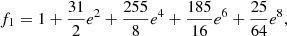
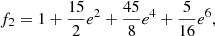
The functions fk can be written as:
 (6)
(6)
 (7)
(7)
 (8)
(8)
 (9)
(9)
 (10)
(10)
For the case of very small initial eccentricities we have:
 (11)
(11)
 (12)
(12)
 (13)
(13)
 (14)
(14)
where
 (15)
(15)
 (16)
(16)
 (17)
(17)
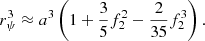
On the other hand, the corresponding theoretical internal structure constants, kj, were computed as a function of time for each component during its evolution through the integration of the differential equations on a Radau order of j:
 (18)
(18)
where
 (19)
(19)
and where a is the mean radius of the equipotential surface within the star, ϵj is the tesseral harmonics of order j, then ρ(a) is the mass density at the distance a from the centre, and  is the mean mass density within an equipotential of radius a. The following boundary conditions were applied: ηj(0) = j − 2, and
 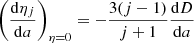 , where
 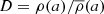 .
.
The moment of inertia was integrated simultaneously using the following equation:
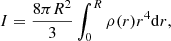 (20)
(20)
where R is the radius of the configuration and ρ(r) the local density. The radius of gyration was computed by using a simple equation:
 (21)
(21)
Equations (11) and (13) were integrated simultaneously through a fifth-order Runge–Kutta method, with a tolerance level of 1 × 10⁻⁷.
3. Tidal evolution of TZ For
The eccentricities of the orbit of TZ For as measured by Andersen et al. (1991), Gallenne et al. (2016) are very similar (0.000 and 0.00002) and so we can assume the orbit to be circular. At this point, we can analyse two possible scenarios: the first one assuming a high initial eccentricity and the other an initially circular system. To get the eccentricity e, Ω1/ω, Ω2/ω and the orbital period as a function of time Eqs. (1)–(4) were integrated using as input the internal structure of theoretical stellar models discussed in Sect. 2.1. A necessary condition for such integrations is knowing the boundary conditions of the differential equations. As explained in Claret (2011), such “observational” initial values are unknown. However, we can introduce some initial test values for the eccentricity, orbital period, and angular velocities to study the tidal evolution. Finally, using this procedure we obtain the evolution of these parameters as a function of time to be compared with their observed counterparts.
The rotational velocity measured by Gallenne et al. (2016) for the secondary component, V2sin i = 45.7 ± 1 km s−1, is not very different from that measured by Andersen et al. (1991), namely: V2sin i = 42 ± 2 km s−1. However, for the primary the rotational velocities given by the authors are 6.1 ± 0.3 km s−1 and 4.0 ± 1, respectively. Here, we adopt the most recent measurements by Gallenne et al. (2016) to obtain the observational ratios Ω1/ω = 1.10 ± 0.03 and Ω2/ω = 17.60 ± 0.03.
3.1. Case of a highly eccentric orbit
As we can verify by inspecting Eqs. (1)–(4), the evolution of the orbital parameters is strongly dependent on the relative radii of the components (eighth and sixth power). At the present evolutionary state of both components of TZ For, the relative radii contribute only slightly to the tidal evolution of the system (around 0.07 and 0.03), respectively. Figure 2 shows the evolution of the orbital period as a function of time for the case of an initial Porb = 80.1 days, einitial = 0.30 and Ω1/ω = Ω2/ω = 21.5. The pronounced peak in the period at log τ = 9.01 (τ represents the time in years) is due to the relative radius of the primary reaching its maximum (≈0.23), while the respective value for the secondary is on the order of only 0.03. Such a peak is statistically very difficult to detect observationally due to the short time interval during which it occurs. From this point on, the period remains practically constant and consistent, within the uncertainties of the stellar models and with its current observational counterpart.
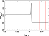 |
Fig. 2. Evolution of the orbital period as a function of time. The two vertical lines indicate the error bars for the mean age of the system. Initial Porb = 80.1 days, einitial = 0.30, and Ω1/ω = Ω2/ω = 21.5. |
A very useful quantity in tidal evolution studies is the timescale (or critical time) for circularisation, or the corresponding log gcri, since it works as a primary diagnostic tool. In the present case, such critical values were computed until the initial eccentricity decayed to 0.368 × einitial. In these calculations, it was assumed that the system is synchronized, namely, Ω1, 2 = ω and einitial = 0.30. Figure 3 illustrates the log gcri or equivalently the time scale as a function of the orbital period (black line). The primary (red square), at the age log τ ≈ 9.01 for which the orbit becomes circularized, is above the critical circularisation curve. On the other hand, the secondary (open star) is below the mentioned curve. This is a preliminary indication of the only slight contribution of the secondary to the circularisation of the orbit. With regard to eccentricity resulting from the integrations of Eqs. (1)–(4), its behaviour is similar to that of the orbital period as shown in Fig. 4, and it also decreases rapidly at log τ ≈ 9.01. On the other hand, several numerical tests reveal that, at least for the case of TZ For, the times for the circularisation of the orbit for these MESA models do not depend strongly on the initial values of the eccentricity.
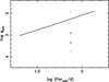 |
Fig. 3. Critical values for circularisation as a function of the orbital period for the case of TZ For (continuous line). The tiny black error bars represent the actual position of the TZ For, the square and the filled star denotes the primary and secondary component, respectively, at the time the system achieves circularisation. |
Concerning the synchronisation of the two components the situation is more complex (Fig. 5). Due to the strong impact of the changes in the radius of the primary in the tidal evolution, this component reaches the synchronism at the same time of stabilisation of the orbital period and of circularisation of the orbit. The effect of the differential evolution is clearly noted since the secondary is relatively far from synchronism given that its angular velocity is approximately 17 times faster than that of the primary component for the age derived for TZ For (log τ ≈ 9.053). Figure 6 shows the orbital period and the rotational velocity of each component as a function of log τ. The respective theoretical values are also in good agreement with the observational data from Gallenne et al. (2016). The spikes in the rotational velocities of the primary and secondary in the intervals of log τ ≈ 9.00–9.013 and 9.050–9.072, respectively, are a consequence of the rapid variations of the surface gravities of both stars (Fig. 6, lower left corner). All these results are in agreement with the observed eccentricity of the system, the measured rotational velocities of both components, and the orbital period considering the intrinsic uncertainties of the evolutionary models (opacities, loss of mass, equation of state, etc.) and the uncertainties in the friction timescale (Sect. 3.3).
 |
Fig. 5. Evolution of the levels of synchronism as a function of time. The angular velocities of the two components were normalized to the mean angular orbital velocity. The continuous line represents the primary and the dashed one denotes the secondary. Same details as in Fig. 2. |
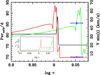 |
Fig. 6. Time evolution of the orbital period (black line) and of the rotational velocities, both primary (red line) and secondary (green line) as well as their respective error bars (blue). The figure in the lower left corner illustrates the variations in the relative radii of the primary and secondary. Same details as in Fig. 2. |
Within this scenario, the nuclear evolution of the primary component is the main activity responsible for the circularisation of the orbit of the system, for the orbital period stabilisation, and also for the primary synchronisation at log τ ≈ 9.01. It remains synchronized until the derived age of TZ For, since its relative radius decreases, thus contributing little to its evolution by tides after the maximum value of the relative radius r1. The case of the secondary component is somewhat different. Despite the small difference in mass, the secondary has a small relative radius at log τ ≈ 9.01 while r1 ≈ 0.23 and therefore the tidal forces are still not sufficient to act on its synchronisation that will occur later, namely, at log τ ≈ 9.065.
3.2. Case of initial circular orbit
The results of the tidal evolution for the case of an initial circular orbit with the following parameters: initial orbital period Porb = 70.0 days, einitial = 0.00, and Ω1/ω = Ω2/ω = 18.2 can be seen in Figs. 7 and 8. Unlike the case with einitial = 0.30, the orbital period increases from 70 to 75 days stabilising at log τ ≈ 9.01. On the other hand, Fig. 8 shows that the angular velocities of the two components present an aspect similar to that of Fig. 5, except for the shape of the peak around log τ ≈ 9.01. The synchronisation times for the two components are approximately the same as those obtained for a very eccentric initial orbit. Taking into account the limitations of the stellar evolutionary models and the friction timescale, tF, we can consider that the theoretical levels of synchronism of both components; although two very different initial conditions have been used, the time evolution of the eccentricity and orbital period are also consistent with their actual observational equivalents at the mean age determined for TZ For.
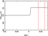 |
Fig. 7. Evolution of the orbital period as a function of time. The two vertical lines indicate the error bars for the mean age of the system. Initial Porb = 70.0 days, einitial = 0.00, and Ω1/ω = Ω2/ω = 18.2. |
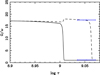 |
Fig. 8. Evolution of the levels of synchronism as a function of time. The continuous line represents the primary and the dashed one denotes the secondary. Same details as in Fig. 7. |
3.3. Influence of the uncertainties of tF on the tidal evolution of TZ For
As we have seen, an acceptable agreement has been achieved between the evolutionary models and the absolute dimensions of TZ For with an error in age < 5%. In the previous section, we show that the tidal theory in the weak friction approach is capable of explaining the current orbital period, the behavior of the eccentricity, and the synchronization levels of the two components. However, one of the weakest points in Eqs. (1)–(4) is the friction time-scale, tF. In this section, we try to estimate the influence of friction time uncertainties on the tidal evolution of TZ For. For this purpose, we adopted a very simple scheme: we assume that the errors in tF are of ±50%. As before, we integrate the aforementioned equations changing tF for the case Pinitial = 80.1 days, einitial = 0.30, and Ω1/ω = Ω2/ω = 21.5 that was taken as the reference.
Figure 9 illustrates the influence of considering errors in tF of ±50% in the evolution of the orbital period where we have taken the results shown in Fig. 2 (black line) as a reference. The differences ΔP/P in the stabilisation zone of the period are respectively 1.4% for the case of [1.5 × tF] and 2.5% for the case of [0.5 × tF]. Such differences are acceptable given the mentioned intrinsic uncertainties in the calculation of the theoretical stellar models. In relation to the evolution of the eccentricity (Fig. 10) the differences in the circularisation times are almost indistinguishable for the three configurations.
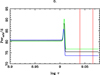 |
Fig. 9. Effects on the orbital period due to uncertainties in the friction time scale tF. The black line represents the evolution of the period as in Fig. 2 while the green line denotes the case [1.5 × tF] and the blue one illustrates the case [0.5 × tF]. Same initial conditions as in Fig. 2. |
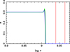 |
Fig. 10. Effects on the eccentricity due to uncertainties in the friction time scale tF. The black line represents the evolution of the eccentricity as in Fig. 3 while the green line denotes the case [1.5 × tF] and the blue one illustrates the case [0.5 × tF]. Same initial conditions as in Fig. 2. |
The evolution of normalized angular velocities is more complex than the case of eccentricity (see Fig. 11) since they present the greatest differences. For example, the values of the normalized rotational velocities of the secondary, considering the mean age of TZ For, differ up to 6% and 14% for [1.5 × tF] and [0.5 × tF], respectively.
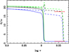 |
Fig. 11. Effects on the levels of synchronism of TZ For due to uncertainties in the friction time scale tF. The black line represents the evolution of angular velocities as shown in Fig. 5, while the green line denotes the case of [1.5 × tF] and the blue one illustrates the case of [0.5 × tF]. The continuous lines denote the primary component and the dashed ones the secondary. The error bars are represented in red. Same initial conditions as in Fig. 2. |
We also note that for a 50% larger value of tF, the normalized angular velocities are approximately equal to or larger than those of the reference model; the opposite occurs reducing by a half tF. It is also remarkable that in both cases, the synchronization times for the two components converge to log τ ≈ 9.01 and 9.065, respectively, even though the normalised angular velocities are different before this time. We can consider that despite assuming uncertainties in tF on the order of 50% and also considering the intrinsic uncertainties in the evolutionary models, the synchronization levels of the two components, the circularisation time, and the stabilization time of the orbital period are compatible with their observational counterparts.
3.4. Another hypothetical scenario: Estimation of the role of rotating models
The fact that the current orbital period of TZ For is long implies some peculiarities. The behaviour of the orbital period (Figs. 2, 7 and 9) shows very accentuated changes in this variable during only a short interval of time (log τ ≈ 9.01). Such rapid changes practically govern the tidal evolution of the system due to the impact of the changes in the relative radii, k2, and the moments of inertia, mainly in the case of the primary component. Outside this short interval of time the orbital period remains practically constant. Of course, there are many more theoretical scenarios that we have on hand to explain the current state of TZ For’s orbital elements, beyond those presented in Sects. 3.1– 3.3. Here, we try to address one of these, which is focused on rotation. In fact, a rotating stellar model evolves differently from a standard one. The differences will be larger if additional phenomena, such as turbulent diffusion, core overshooting, or rotational-mixing, are taken into account. The evolution of a rotating model will differ from the standard one in terms of luminosity, effective temperatures, lifetimes of Hydrogen and He burning, and changes in the surface chemical abundances, as well as its internal structure (k2 and β). Differently from the results presented in the previous sections, we investigate here the role of rotating models in the evolution of the orbital elements of TZ For. For this purpose, we introduced rotation in the GRANADA code using the method by Kippenhahn & Thomas (1970), improved by Endal & Sofia (1976, 1978) and adapted in this code by Claret (1999). Such a code is designed to treat systems disturbed by rotation and by tidal forces. To take into account only the effects of rotation, we assumed the mass ratio to be q = 0. We adopted the solid body and overall conservation of angular momentum approach for simplicity. However, such rotating models present some limitations: by definition, in such models, the angular velocity is the same throughout the model. Another important simplification is that rotational mixing has not been considered (only core overshooting is taken into account). These simplifications limit the scope of our conclusions, but they allow us to estimate the effects of the departure from spherical geometry on k2 and on the radius of gyration which are key for the tidal evolution calculations.
In searching for the best solution, we used the same method and the statistics χ2 described above for the MESA models, also taking into account the grids of initial angular velocities. The input physics for the best solution for the rotating models was: X = 0.711, Z = 0.015, αMLT1 = 1.82, αMLT2 = 1.82, αov1 = 0.23, and αov2 = 0.21. The adopted opacities are based on the mixture of Asplund et al. (2009). We note that convective core overshooting in the GRANADA code is simulated adopting a step-function, characterized by the parameter αov whose relation with fov is given by αov/fov = 11.36 ± 0.22 following Claret & Torres (2017). The initial angular velocities were Ω1 = 5.2 × 10⁻⁵ s−1 and Ω2 = 4.9 × 10⁻⁵ s−1. The rotacional velocities of both components reaching the ZAMS (zero age main sequence) are 84.0 and 77.0 km s−1, respectively. These values are compatible with the observational data for DLEBS with similar masses, as for example, the case of V1647 Sgr, whose observational counterparts are, respectively, 80 ± 5 km s−1 and 77 ± 5 km s−1 (Torres et al. 2010, Table 2). The derived common age was 1.23 ± 0.05 Gyr. The difference between the ages of TZ For as derived using the MESA and GRANADA codes are due mainly to the different nuclear network adopted in both codes (see Claret 2004, Sect. 2). Furthermore, the introduction of rotation also influences the determination of the ages. For details on the implementation of rotation in GRANADA models, we refer to Appendix A.
The results of these calculations can be seen in Fig. 12, where the rotational velocities are represented as a function of log g. As it can be inspected in such a figure, the theoretical values of the rotational velocities are in good agreement with their observational counterparts. In such a figure, it can be verified that both components of TZ For are in the same evolutionary stages as in the case shown in Fig. 1. In fact, the corresponding HR Diagram for such models corroborates this point. This similarity indicates that, although the present evolutionary models were computed using a different code and input physics from that discussed in Sect. 2.1, the intercomparison leads to similar results concerning the evolutionary status of TZ For and also the respective internal structure (k2 and moment of inertia). This shows the consistency between the two stellar evolution codes used in the present study, despite the differences in the respective nuclear networks and the implementation of rotation in the GRANADA models.
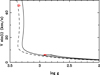 |
Fig. 12. Rotational velocities for TZ For for the case of solid body rotation. Continuous line represents the primary and the dashed one denotes the secondary. The calculations were performed following a revised version of GRANADA code by Claret (1999). The derived mean age of the system is 1.23 ± 0.05 Gyr. |
In order investigate the effects of the intrinsec stellar rotation, we proceeded to calculate the evolution by tides using the rotating GRANADA models. As a novelty, we did not use trial values for the rotational velocities (as we had done in the case of the MESA models). Here, we adopt the initial Ωi derived from GRANADA models with rotation (Fig. 12) as initial conditions. The similarities between Figs. 2, 4, and 5 (MESA) and their corresponding ones using the rotating GRANADA models (Figs. 13–15) are notorious, except for the timescale and the initial orbital period adopted, which is as expected. This fact confirms again that the internal structures of both models are very similar. On the other hand, in Fig. 16 we can see that such a similarity also extends to the rotational velocities. Comparing the rotational velocities shown in Figs. 6 and 16, we note that both are morphologically similar. However, they differ regarding the values being the ones shown in Fig. 16 systematically larger. The reason for this is that in Fig. 16, the adopted initial period is smaller than its counterpart in Fig. 6. In addition, the corresponding angular velocities were computed with initial values of Ωi/ω larger than in the case shown in Fig. 6 (56.0 and 21.5, respectively). In fact, the maximum value of the relative radius of the primary in Fig. 16 is larger than that shown in Fig. 6 (0.25 and 0.23, respectively). This implies, for example, that the tidal interaction is about 2.0 times stronger in the case of Fig. 16 during such maxima.
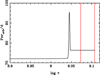 |
Fig. 13. Evolution of the orbital period as a function of time. Initial Porb = 72.03 days, einitial = 0.30, and Ω1/ω = Ω2/ω = 56.0. The initial conditions for the angular velocities of the two components are those of the GRANADA models with rotation near the ZAMS. The two vertical lines indicate the error bars for the mean age of the system. |
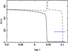 |
Fig. 15. Evolution of the levels of synchronism as a function of time. The continuous line represents the primary and the dashed one denotes the secondary. Same details as in Fig. 13. |
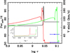 |
Fig. 16. Rotational velocities, according to the integrations of Eqs. (1)–(4), as a function of time for the rotating models shown in Fig. 12. Continuous red line represents the primary and the green one denotes the secondary. The two blue lines indicate the error bars for the mean age of the system. Lower-left corner illustrates the variations in the relative radii of the primary and secondary. Same initial conditions as in Fig. 13. |
3.5. Summary
We studied the nuclear and tidal evolution of the TZ For system using evolutionary tracks computed with two different codes. Such models reproduce, within the observational errors, the absolute dimensions of the system with a tolerance of 5% in the common age.
Regarding tidal evolution, we integrated the equations of Hut (1981) in the cases of high (0.30) and low (0.0) initial eccentricities. Good agreement has been found between the observed values of eccentricity, orbital period, and synchronism levels with their theoretical counterparts. The influence of friction time in such calculations was also studied and we have concluded that its influence affects the synchronization levels of both components is greater, although we consider that they are acceptable given the intrinsic uncertainties in tF and in the stellar evolutionary models.
On the other hand, we computed rotating evolutionary tracks with the code GRANADA. Such models, which also reproduce the absolute dimensions of TZ For, were used to estimate the influence of rotating models on tidal evolution. For this purpose, we used the theoretical initial angular velocities of the two components as the initial conditions for the integrations of Eqs. (1)–(4). These values do not replace the observational values for which we do not have reliable data so far, but we believe it is a small step forward. As in the previous cases, we found a good agreement between the observed orbital elements and their corresponding theoretical values.
Acknowledgments
I thank an anonymous referee for his/her careful reading of the original version as well as for his/her comments and suggestions. The Spanish MEC (ESP2017-87676-C5-2-R, PID2019-107061GB-C64, and PID2019-109522GB-C52) is gratefully acknowledged for its support during the development of this work. A.C. acknowledges financial support from the State Agency for Research of the Spanish MCIU through the “Center of Excellence Severo Ochoa” award for the Instituto de Astrofísica de Andalucía (SEV-2017-0709). This research has made use of the SIMBAD database, operated at the CDS, Strasbourg, France, and of NASA’s Astrophysics Data System Abstract Service.
References
- Ade, P. A. R., Aghanim, N., Arnaud, M., et al. 2016, A&A, 594, A13 [NASA ADS] [CrossRef] [EDP Sciences] [Google Scholar]
- Andersen, J., Clausen, J. V., Nordstrom, B., Tomkin, J., & Mayor, M. 1991, A&A, 246, 99 [NASA ADS] [Google Scholar]
- Asplund, M., Grevesse, N., Sauval, A. J., & Scott, P. 2009, ARA&A, 47, 481 [NASA ADS] [CrossRef] [Google Scholar]
- Böhm-Vitense, E. 1958, Z. Astrophys., 46, 108 [Google Scholar]
- Claret, A. 1999, A&A, 350, 56 [NASA ADS] [Google Scholar]
- Claret, A. 2004, A&A, 424, 919 [NASA ADS] [CrossRef] [EDP Sciences] [Google Scholar]
- Claret, A. 2011, A&A, 526, A157 [NASA ADS] [CrossRef] [EDP Sciences] [Google Scholar]
- Claret, A., & Cunha, N. C. S. 1997, A&A, 318, 187 [NASA ADS] [Google Scholar]
- Claret, A., & Giménez, A. 1995, A&A, 296, 180 [NASA ADS] [Google Scholar]
- Claret, A., & Torres, G. 2016, A&A, 592, A15 [NASA ADS] [CrossRef] [EDP Sciences] [Google Scholar]
- Claret, A., & Torres, G. 2017, ApJ, 849, 18 [Google Scholar]
- Claret, A., & Torres, G. 2018, ApJ, 859, 100 [Google Scholar]
- Claret, A., & Torres, G. 2019, ApJ, 876, 134 [Google Scholar]
- Costa, G., Girardi, L., Bressan, A., et al. 2019, MNRAS, 485, 4641 [NASA ADS] [CrossRef] [Google Scholar]
- Endal, A. S., & Sofia, S. 1976, ApJ, 210, 184 [NASA ADS] [CrossRef] [Google Scholar]
- Endal, A. S., & Sofia, S. 1978, ApJ, 220, 279 [NASA ADS] [CrossRef] [Google Scholar]
- Freytag, B., Ludwig, H.-G., & Steffen, M. 1996, A&A, 313, 497 [Google Scholar]
- Gallenne, A., Pietrzyñski, G., Graczyk, D., et al. 2016, A&A, 586, 35 [NASA ADS] [Google Scholar]
- Grevesse, N., & Sauval, A. J. 1998, SSRv, 85, 161 [NASA ADS] [Google Scholar]
- Herwig, F., Bloecker, T., Schoenberner, D., & El Eid, M. 1997, A&A, 324, L81 [NASA ADS] [Google Scholar]
- Hut, P. 1981, A&A, 99, 126 [NASA ADS] [Google Scholar]
- Kippenhahn, R., & Thomas, R. C. 1970, in Stellar Rotation, ed. A. Slettebak (Dordrecht, Holland: D. Reidel Publ. Co.), 20 [CrossRef] [Google Scholar]
- Kopal, Z. 1959, Close Binary Systems (London: Chapman& Hall) [Google Scholar]
- Paxton, B., Bildsten, L., Dotter, A., et al. 2011, ApJS, 192, 3 [Google Scholar]
- Paxton, B., Cantiello, M., Arras, P., et al. 2013, ApJS, 208, 4 [Google Scholar]
- Paxton, B., Marchant, P., Schwab, J., et al. 2015, ApJS, 220, 15 [Google Scholar]
- Reimers, D. 1977, A&A, 61, 217 [NASA ADS] [Google Scholar]
- Rieutord, M. 1992, A&A, 259, 581 [Google Scholar]
- Tassoul, J. L. 1987, ApJ, 322, 856 [NASA ADS] [CrossRef] [Google Scholar]
- Tassoul, J. L., & Tassoul, M. 1996, Fundament. Cosmic Phys., 16, 337 [NASA ADS] [Google Scholar]
- Torres, G., Andersen, J., & Giménez, A. 2010, A&ARv, 18, 67 [Google Scholar]
Appendix A: Brief description of the numerical method for computing stellar rotating models
The formalism by Kippenhahn & Thomas (1970) has been used to simulate the effects of the stellar rotation on the internal density concentration as well as on the evolution of the rotational velocity. The mathematical basis of this method can be found in Kippenhahn & Thomas (1970) and improved by Endal & Sofia (1976, 1978). A star distorted by rotation and by tides is represented by a Roche’s critical surface. The suitable potential is written in terms of massratio, relative distance and angular velocities. This potential presents some advantages, as for example: if the only interest is to investigate the effects of stellar rotation, then the mass ratio ought to be q = 0.0.
To simulate rotating stars we restricted the calculation to first order theory and the total potential can be written as given by Kopal (1959):
 (A.1)
(A.1)
where
 (A.2)
(A.2)
 (A.3)
(A.3)
In the above equations Ω is the angular velocity, P2(cos θ) is the second Legendre polynomial, a the radius of the level surface, η2 is the solution of the Radau’s equation (Eq. 11), and the remaining symbols retain their usual meaning.
In this framework a generic function F(r, θ, ϕ) has its counterpart according to:
 (A.4)
(A.4)
where dS is the element of surface for constant values of ψ. On the other hand, the effective gravity is given by:
 (A.5)
(A.5)
where dn is the distance between two neighbouring surfaces.
The corresponding volume of the configuration is thus given by:
 (A.6)
(A.6)
The usual differential equations of the stellar structure are changed to:
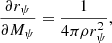 (A.7)
(A.7)
 (A.8)
(A.8)
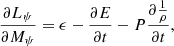 (A.9)
(A.9)
 (A.10)
In the above equations, Mψ, Lψ are the mass and luminosity enclosed by a constant equipotential, ϵ is the nuclear energy generation rate per unit mass, E is the internal energy per unit of mass, T and P the temperature and pressure, ρ the density, a the radiation pressure constant (not to be confused with mean radius of an equipotential), and c the velocity of light in vacuum. In principle, when using these approximations, it would be necessary to solve the Poisson equation simultaneously. We note that if we choose the potential as the solution corresponding to the Roche model, such a condition is not necessary.
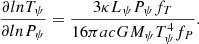
After some algebra the Schwarzschild criterion can be written as:
![Mathematical equation: $$ \begin{aligned} {\partial ln T_{\psi }\over {\partial ln P_{\psi }}} = min [ \bigtriangledown _{ad}, {\bigtriangledown _{rad}}{f_{T}\over {f_P}}], \end{aligned} $$](/articles/aa/full_html/2022/08/aa43573-22/aa43573-22-eq35.gif) (A.11)
(A.11)
where ▽ad and ▽rad are the "spherical" adiabatic and radiative gradients. The variables fP and fT are computed following the equations:
 (A.12)
and
 (A.13)
The functions fP and fT depend on the shape of the equipotential surfaces and for fP and fT = 1.0 that we recover the spherical model. To simulate rotating models we have used an updated version of the GRANADA code described in Claret in 1999 (and revised in 2022). Inspecting Eqs. A1-A3, we note that Eq. 11 should be integrated simultaneously to obtain η2 at each point of the model to solve the modified differential equations of stellar structure. This is also necessary for the calculation of average local gravity and its inverse. Regarding the numerical method used to calculate the rotating models we introduced the following procedure to take into account these requirements: the first model is computed without rotation. It will give, through integrations, the values of η2 and therefore of the integral in Eq. A1 for each point to be used in a second model which includes rotation. For this second model (and all the following ones), the values of the integral and of η2 will include the rotational effects. The model n will be computed considering the values of the integral and of η2 as derived from the model n − 1. Provided that neighboring models have similar structures (small steps in time) the method guarantees a good accuracy. Finally, to compute fP and fT, we need to use a relationship between rψ and the mean radius of a given equipotential a. Such variables are connected by the following equation which is solved by iteration:
 (A.14)
For more detailed information on the implementation of rotation in the GRANADA code, we refer to Claret (1999).
All Figures
|
Fig. 1. HR diagram for TZ For. The models were calculated adopting Z = 0.015. Solid line indicates the primary component while the dashed one represents the secondary. |
| In the text | |
|
Fig. 2. Evolution of the orbital period as a function of time. The two vertical lines indicate the error bars for the mean age of the system. Initial Porb = 80.1 days, einitial = 0.30, and Ω1/ω = Ω2/ω = 21.5. |
| In the text | |
|
Fig. 3. Critical values for circularisation as a function of the orbital period for the case of TZ For (continuous line). The tiny black error bars represent the actual position of the TZ For, the square and the filled star denotes the primary and secondary component, respectively, at the time the system achieves circularisation. |
| In the text | |
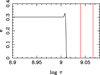 |
Fig. 4. Evolution of the eccentricity as a function of time. Same details as in Fig. 2. |
| In the text | |
|
Fig. 5. Evolution of the levels of synchronism as a function of time. The angular velocities of the two components were normalized to the mean angular orbital velocity. The continuous line represents the primary and the dashed one denotes the secondary. Same details as in Fig. 2. |
| In the text | |
|
Fig. 6. Time evolution of the orbital period (black line) and of the rotational velocities, both primary (red line) and secondary (green line) as well as their respective error bars (blue). The figure in the lower left corner illustrates the variations in the relative radii of the primary and secondary. Same details as in Fig. 2. |
| In the text | |
|
Fig. 7. Evolution of the orbital period as a function of time. The two vertical lines indicate the error bars for the mean age of the system. Initial Porb = 70.0 days, einitial = 0.00, and Ω1/ω = Ω2/ω = 18.2. |
| In the text | |
|
Fig. 8. Evolution of the levels of synchronism as a function of time. The continuous line represents the primary and the dashed one denotes the secondary. Same details as in Fig. 7. |
| In the text | |
|
Fig. 9. Effects on the orbital period due to uncertainties in the friction time scale tF. The black line represents the evolution of the period as in Fig. 2 while the green line denotes the case [1.5 × tF] and the blue one illustrates the case [0.5 × tF]. Same initial conditions as in Fig. 2. |
| In the text | |
|
Fig. 10. Effects on the eccentricity due to uncertainties in the friction time scale tF. The black line represents the evolution of the eccentricity as in Fig. 3 while the green line denotes the case [1.5 × tF] and the blue one illustrates the case [0.5 × tF]. Same initial conditions as in Fig. 2. |
| In the text | |
|
Fig. 11. Effects on the levels of synchronism of TZ For due to uncertainties in the friction time scale tF. The black line represents the evolution of angular velocities as shown in Fig. 5, while the green line denotes the case of [1.5 × tF] and the blue one illustrates the case of [0.5 × tF]. The continuous lines denote the primary component and the dashed ones the secondary. The error bars are represented in red. Same initial conditions as in Fig. 2. |
| In the text | |
|
Fig. 12. Rotational velocities for TZ For for the case of solid body rotation. Continuous line represents the primary and the dashed one denotes the secondary. The calculations were performed following a revised version of GRANADA code by Claret (1999). The derived mean age of the system is 1.23 ± 0.05 Gyr. |
| In the text | |
|
Fig. 13. Evolution of the orbital period as a function of time. Initial Porb = 72.03 days, einitial = 0.30, and Ω1/ω = Ω2/ω = 56.0. The initial conditions for the angular velocities of the two components are those of the GRANADA models with rotation near the ZAMS. The two vertical lines indicate the error bars for the mean age of the system. |
| In the text | |
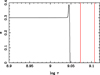 |
Fig. 14. Evolution of the eccentricity as a function of time. Same details as in Fig. 13. |
| In the text | |
|
Fig. 15. Evolution of the levels of synchronism as a function of time. The continuous line represents the primary and the dashed one denotes the secondary. Same details as in Fig. 13. |
| In the text | |
|
Fig. 16. Rotational velocities, according to the integrations of Eqs. (1)–(4), as a function of time for the rotating models shown in Fig. 12. Continuous red line represents the primary and the green one denotes the secondary. The two blue lines indicate the error bars for the mean age of the system. Lower-left corner illustrates the variations in the relative radii of the primary and secondary. Same initial conditions as in Fig. 13. |
| In the text | |
Current usage metrics show cumulative count of Article Views (full-text article views including HTML views, PDF and ePub downloads, according to the available data) and Abstracts Views on Vision4Press platform.
Data correspond to usage on the plateform after 2015. The current usage metrics is available 48-96 hours after online publication and is updated daily on week days.
Initial download of the metrics may take a while.