| Issue |
A&A
Volume 664, August 2022
|
|
|---|---|---|
| Article Number | A65 | |
| Number of page(s) | 21 | |
| Section | Planets and planetary systems | |
| DOI | https://doi.org/10.1051/0004-6361/202142828 | |
| Published online | 10 August 2022 | |
HADES RV Programme with HARPS-N at TNG
XV. Planetary occurrence rates around early-M dwarfs★,★★
1
INAF – Osservatorio Astrofisico di Torino,
Via Osservatorio 20,
10025
Pino Torinese, Italy
e-mail: This email address is being protected from spambots. You need JavaScript enabled to view it.
2
INAF – Osservatorio Astronomico di Palermo,
piazza del Parlamento 1,
90134
Palermo, Italy
3
INAF – Osservatorio Astrofisico di Catania,
Via S. Sofia 78,
95123
Catania, Italy
4
Institut de Ciències de l’Espai (ICE, CSIC),
Campus UAB, C/ de Can Magrans s/n,
08193
Bellaterra, Spain
5
Institut d’Estudis Espacials de Catalunya (IEEC),
C/ Gran Capità 2-4,
08034
Barcelona, Spain
6
Instituto de Astrofísica de Canarias (IAC),
38205
La Laguna, Tenerife, Spain
7
Universidad de La Laguna,
Dpto. Astrofísica,
38206
La Laguna, Tenerife, Spain
8
INAF – Osservatorio Astronomico di Trieste,
via G. B. Tiepolo 11,
34143
Trieste, Italy
9
INAF – Osservatorio Astronomico di Padova,
vicolo dell’Osservatorio 5,
35122
Padova, Italy
10
INAF – Osservatorio Astronomico di Capodimonte,
Salita Moiariello 16,
80131
Napoli, Italy
11
Centro de Astrobiología (CSIC-INTA),
Carretera de Ajalvir km 4,
28850
Torrejón de Ardoz, Madrid, Spain
12
INAF – Osservatorio Astronomico di Cagliari & REM,
Via della Scienza, 5,
09047
Selargius CA, Italy
13
Dipartimento di Fisica e Astronomia, Università di Padova,
via Marzolo 8,
35131
Padova, Italy
14
Fundación Galileo Galilei - INAF,
Ramble José Ana Fernandez Pérez 7,
38712
Breña Baja, TF, Spain
15
INAF – Osservatorio Astronomico di Brera,
via E. Bianchi 46,
23807
Merate, Italy
Received:
3
December
2021
Accepted:
28
February
2022
Abstract
Aims. We present the complete Bayesian statistical analysis of the HArps-n red Dwarf Exoplanet Survey (HADES), which monitored the radial velocities of a large sample of M dwarfs with HARPS-N at TNG over the last 6 yr.
Methods. The targets were selected in a narrow range of spectral types from M0 to M3, 0.3 M⊙ < M★ < 0.71 M⊙, in order to study the planetary population around a well-defined class of host stars. We take advantage of Bayesian statistics to derive an accurate estimate of the detectability function of the survey. Our analysis also includes the application of a Gaussian Process approach to take into account stellar-activity-induced radial velocity variations and improve the detection limits around the most-observed and most-active targets. The Markov chain Monte Carlo and Gaussian process technique we apply in this analysis has proven very effective in the study of M-dwarf planetary systems, helping the detection of most of the HADES planets.
Results. From the detectability function we can calculate the occurrence rate of small-mass planets around early-M dwarfs, either taking into account only the 11 already published HADES planets or adding the five new planetary candidates discovered in this analysis, and compare them with the previous estimates of planet occurrence around M-dwarf or solar-type stars: considering only the confirmed planets, we find the highest frequency for low-mass planets (1 M⊕ < mp sin i < 10 M⊕) with periods 10 d < P < 100 d,  , while for short-period planets (1 d < P < 10 d) we find a frequency of
  , significantly lower than for later-M dwarfs; if instead we also take into account the new candidates, we observe the same general behaviours, but with consistently higher frequencies of low-mass planets. We also present new estimates of the occurrence rates of long-period giant planets and temperate planets inside the habitable zone of early-M dwarfs: in particular we find that the frequency of habitable planets could be as low as η⊕ < 0.23. These results, and their comparison with other surveys focused on different stellar types, confirm the central role that stellar mass plays in the formation and evolution of planetary systems.
Key words: techniques: radial velocities / stars: low-mass / stars: activity / methods: statistical / planets and satellites: detection
All RV and activity data are only available at the CDS via anonymous ftp to cdsarc.u-strasbg.fr (130.79.128.5) or via http://cdsarc.u-strasbg.fr/viz-bin/cat/J/A+A/664/A65
Based on: observations made with the Italian Telescopio Nazionale Galileo (TNG), operated on the island of La Palma by the INAF – Fundación Galileo Galilei at the Roque de Los Muchachos Observatory of the Instituto de Astrofísica de Canarias (IAC); photometric observations made with the APACHE array located at the Astronomical Observatory of the Aosta Valley; photometric observations made with the robotic telescope APT2 (within the EXORAP programme) located at Serra La Nave on Mt. Etna.
© ESO 2022
1 Introduction
Due to the many observational advantages facilitating the detection of rocky planets in close orbits around them, M dwarfs have become increasingly popular as targets for extrasolar planet searches (e.g. Dressing & Charbonneau 2013; Sozzetti et al. 2013; Astudillo-Defru et al. 2017). However, these advantages are counterweighted by the difficulties in both detection and characterisation of exoplanetary systems caused by the stellar activity of the host stars, which can produce radial velocity (RV) signals comparable to those from actual planets, leading to possible misinterpretations (e.g. Bonfils et al. 2007; Robertson et al. 2014; Anglada-Escudé et al. 2016). Moreover, M-dwarf planetary systems offer an interesting laboratory to test planet formation theories, because they form under different conditions with respect to FGK-dwarf systems, with different proto-planetary disk masses, temperature, and density profiles, and gas-dissipation timescales (e.g. Ida & Lin 2005).
Several previous studies attempted to compute the occurrence rate of extrasolar planets of different kinds around low-mass stars, taking into account the detection biases of different surveys. Bonfils et al. (2013) analysed the M dwarf sample observed as part of the RV search for southern extrasolar planets with the ESO/HARPS spectrograph (Mayor et al. 2003). Tuomi et al. (2014) studied a similar though smaller sample of M dwarfs observed with both the HARPS and UVES spectrographs (Dekker et al. 2000). The statistical properties of exoplanets in the Kepler M dwarfs sample were analysed by several authors; for example Dressing & Charbonneau (2015) and Gaidos et al. (2016). Their general results pointed towards a high number of low-mass planets orbiting at different distances from their hosts, and confirmed the paucity of giant planets already suggested by earlier surveys (Endl et al. 2003, 2006; Cumming et al. 2008). Recently, Sabotta et al. (2021) computed the occurrence rates from a subsample of 71 stars observed within the CARMENES exoplanet survey. Their sample covered a wide range of host-star masses between 0.09 M⊙ and 0.70 M⊙, and found slightly higher occurrence rates, although compatible with those from Bonfils et al. (2013).
In this framework, the Harps-n red Dwarf Exoplanet Survey (HADES, Affer et al. 2016) programme aims to fully characterise the population of exoplanetary systems on a consistent sample of stars with well-known properties in order to minimise the effects of varying stellar properties on the planetary frequency measurements. To this end, a catalogue of early-M dwarfs in a narrow range of stellar masses was selected. HADES is a collaboration between the Italian Global Architecture of Planetary Systems (GAPS, Covino et al. 2013; Desidera et al. 2013; Poretti et al. 2016) Consortium, the Institut de Ciències de l’Espai de Catalunya (ICE), and the Instituto de Astrofísica de Canarias (IAC). Perger et al. (2017a) carried out a performance study of the survey based on the first 4 yr of HADES observations: these authors performed a simulation analysis based on the expected population of early-M planets, and predicted a yield of significant detections of 2.4 ± 1.5 planets over the whole sample. However, the results of Perger et al. (2017a) were based on the number of observations collected at that time, which more than doubled by the end of the survey (see Sect. 2). Following the same assumptions, in their Fig. 13 these latter authors derived the expected yields of planets for different numbers of targets and observations per target. We can therefore derive the expected number of detected planets corresponding to the final number of HADES observations, that is, 3.8 ± 1.9 planets. To date, 11 planets have been detected as part of the survey (Affer et al. 2016, 2019; Suárez Mascareño et al. 2017; Perger et al. 2017b, 2019; Pinamonti et al. 2018, 2019; Toledo-Padrón et al. 2021; González-Álvarez et al. 2021; Maldonado et al. 2021), which is already exceeding more than 3σ from the adjusted prediction. This shows how the previous knowledge of early-M dwarf planetary populations was incomplete. Moreover, during recent years, advanced techniques to mitigate stellar noise have been adopted, further improving the detection limits of RV surveys, and increasing the yield of detected planets. The published HADES planets are shown in Fig. 1. Moreover, in Pinamonti et al. (2019) we studied the population of extrasolar planets orbiting M dwarfs detected using the RV technique. We found moderate evidence of a correlation between planetary mass and stellar metallicity, with different behaviours for small and large planets, which is expected from theory (e.g. Mordasini et al. 2012). In Maldonado et al. (2020), we analysed a large sample of M dwarfs in a homogeneous way, and confirmed that giant planet frequency exhibits a correlation with metallicity, while the same does not seem to be true for low-mass planets; these trends are similar to those previously observed for FGK stars (e.g. Sousa et al. 2008; Adibekyan et al. 2012). Pinamonti et al. (2019) also confirmed the effect pointed out by Luque et al. (2018) of different mass distributions between single and multiple planetary systems. However, these studies were conducted over a heterogeneous sample of planets detected from different surveys, which could not be corrected for detection biases. Therefore, their results are to be considered preliminary, because observational biases may have a strong influence on the observed distributions.
In this work, we present a thorough Bayesian characterisation of the HADES planetary population statistics and global detectability of the survey. We model our analysis on the Bayesian approach proposed by Tuomi et al. (2014). We implement this technique with the Monte Carlo Markov chain (MCMC) and Gaussian Process (GP) regression framework, which we successfully applied in the detection of several of the planetary systems of the survey (e.g. Affer et al. 2016; Pinamonti et al. 2018, 2019).
In Sect. 2, we describe the HADES programme and summarise the characteristics of its targets. In Sect. 3, we detail the MCMC analysis technique and main results in the identification of planetary signals, while in Sect. 4 we discuss the detection limits of the survey derived from our Bayesian analysis. In Sect. 5, we discuss the planetary occurrence rates we derive for early M dwarfs, and in Sect. 6, we compare them with previous results of similar surveys and also with the statistics of FGK-dwarf systems. We summarise our conclusions in Sect. 7.
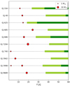 |
Fig. 1 Overview of the HADES detected planetary systems. The published planets of the sample are shown as red circles: the symbol size is proportional to the minimum planetary mass. The conservative and optimistic limits of the habitable zone of each system (see Sect. 5.1) are shown as thick dark green and light green bands, respectively. |
2 The survey
As discussed in Affer et al. (2016), the initial HADES sample was constructed by selecting 106 targets from the Lépine & Gaidos (2013) and PMSU (Palomar/Michigan State University, Reid et al. 1995) catalogues: the stars were required to have spectral types between M0 and M3, with masses between 0.3 M⊙ and 0.7 M⊙, a visual magnitude V < 12, and both to have a high number of Gaia mission (Gaia Collaboration 2016) visits and to be part of the target catalogue of the photometric survey APACHE (A PAthway towards the CHaracterization of Habitable Earths, Sozzetti et al. 2013). Several targets were successively discarded, as they were discovered to be ill-suited to planet searches because of close binary companions, fast rotation (v sin i > 4 km s−1), very high chromospheric activity levels (log R’HK > −4.3), incorrect spectral type (Teff > 4000 K), or for having been classified as subgiants/giants (log ɡ < 4). All the stellar parameters of the targets were consistently re-derived by Maldonado et al. (2017) from the HADES HARPS-N measurements by applying the techniques from Maldonado et al. (2015), which allowed precise estimates of spectral types, metallicities, and effective temperatures. For the current study, we also selected only targets that were observed at least ten times, because with fewer observations our Bayesian analysis technique discussed in Sect. 3 could not be robustly applied.
Applying the aforementioned selection criteria, the HADES sample was reduced to 56 targets, with spectral types between M0 and M3. The parameters important for this analysis of all the stars in the sample, as computed by Maldonado et al. (2020), are listed in Table 1. The RVs were derived with the Template-Enhanced Radial velocity Re-analysis Application (TERRA, Anglada-Escudé & Butler 2012): this template-matching approach has proven to be more effective than the CCF technique of the standard HARPS-N Data Reduction System pipeline (DRS, Lovis & Pepe 2007), in particular in the analysis of early-M dwarf spectra (Affer et al. 2016; Perger et al. 2017a). Moreover, we computed the TERRA RVs considering only spectral orders redder than the 22nd (λ > 453 nm)1 in order to avoid the low-signal-to-noise-ratio (S/N) blue part of the M dwarfs spectra. The observations were carried out from August 2012 to December 2018, with an average time-span 〈Ts〉 = 1760 d (median 1890 d). The average number of RVs per target is 77 (median 60), which is more than twice the average number of observations collected at the time of the performance study by Perger et al. (2017a). Moreover, it is worth noting that this typical number of observations per target is significantly larger than the average number of observations used by Bonfils et al. (2013) (20), and Tuomi et al. (2014) (62). All RV and activity data used in this analysis are available at the CDS in machine-readable format.
Stellar rotation periods
Stellar surface inhomogeneities often produce RV signals close to the rotation period of the star, which can easily mimic the planetary signals (e.g. Vanderburg et al. 2016). This is particularly significant around M dwarfs, because these stellar signals have periods and amplitudes comparable to those of rocky planets in the habitable zone of their stars (Newton et al. 2016). For these reasons, several studies attempted to obtain a precise characterisation of the stellar rotation periods and activity features of the HADES sample: Maldonado et al. (2017) and Scandariato et al. (2017) studied the activity indicator behaviour in the M dwarf sample monitored by the HADES programme, identifying many useful relationships between activity, rotation, and stellar emission lines; González-Álvarez et al. (2019) studied the X-ray luminosity as a proxy of the coronal activity of the stars in the sample, and its relationship with the stellar rotation periods. Suárez Mascareño et al. (2018) instead used spectral activity indicators and photometry to investigate the presence of signatures of rotation and magnetic cycles in 71 HADES M dwarfs, providing activity-index derived rotation periods for 33 of those stars and 36 rotation periods estimated from activity—rotation relationships. All the 33 targets with activity-derived rotation periods are included in the sample of the current analysis, along with 23 of those with periods derived from activity relationships. The relevant rotation periods are listed in Table 1. Moreover, 23 HADES targets have photometric rotation periods detected in the APACHE light curves (Giacobbe et al. 2020), which shows a good correspondence with the spectroscopically derived rotation periods, being either equal or with one close to the first harmonic of the other.
This information over the stellar rotation periods of the sample is very important for our study, because it is paramount to the identification of real Keplerian and activity-induced RV variation during the Bayesian modelling of the time series, as discussed in Sect. 3.4. It is worth noting that, in the analysis of the impact of activity, the active region lifetime is also an important parameter (e.g. Giles et al. 2017; Damasso et al. 2019); however, as not all of our stars have time-series that are sufficiently well sampled for the application of sophisticated analysis techniques such as GP regression, we focus on the rotation period as the main parameter for stellar activity modelling.
3 MCMC analysis
3.1 Statistical analysis technique
Our analysis technique follows the approach by Tuomi et al. (2014), who used Bayesian statistics to estimate the occurrence rate and detectability function of extrasolar planets around M dwarfs.
For each time-series of the sample, the observed number of planets in a given period-mass interval ΔP,M can be expressed as:
 (1)
(1)
where the subscript i indicates the ith system: focci is the occurrence rate of planets around the ith star, and pi is the detectability function, that is, the probability of detecting a planet in the parameter interval ΔP,M in the ith time -series. fobs,i is simply computed as the number of planets detected from each time-series in each parameter interval.
Assuming that ki Keplerian signals were detected in the ith dataset, the Bayesian technique from Tuomi et al. (2014) estimates the detectability function pi by applying a ki + 1-signals model to the time-series by means of a sampling algorithm. This way, the region of the (P, M) parameter space explored by the parameters of the hypothetical k + 1th test-planet, which cannot be significantly detected in the data, represents the region of the parameter space where the detection technique is not able to reveal significant signals, that is, the RV amplitudes are so low that the likelihood function does not rule out the presence of a hypothetical additional planetary signal. More precisely, the areas that were not explored by the Markov chains are the areas where signal detection could have been possible, if significant signals were actually present in the data. The detectability function can therefore be approximated as:
 (2)
(2)
where  is equal to one in the regions of parameters space explored by the k + 1th Keplerian, and zero otherwise (as detailed in Sect. 3.2.2). An example of the detection function pi derived with this method is shown in Fig. 2 for the planet-hosting star GJ 15 A (Pinamonti et al. 2018).
The observed frequency of planets in a given range of orbital period and planetary mass over the whole sample of N datasets can be computed by the sum over i of Eq. (1):
![Mathematical equation: $\matrix{ {{f_{{\rm{obs}}}}\left( {{{\rm{\Delta }}_{{\rm{P,M}}}}} \right)} \hfill & { = \mathop \sum \limits_{i = 1}^N {f_{{\rm{obs,}}i}}\left( {{{\rm{\Delta }}_{{\rm{P,M}}}}} \right)} \hfill \cr {} \hfill & { = {f_{{\rm{occ}}}}\left( {{{\rm{\Delta }}_{{\rm{P,M}}}}} \right)\left[ {N - \mathop \sum \limits_{i = 1}^N {{\hat p}_i}\left( {{{\rm{\Delta }}_{{\rm{P,M}}}}} \right)} \right],} \hfill \cr }$](/articles/aa/full_html/2022/08/aa42828-21/aa42828-21-eq6.png) (3)
(3)
assuming the occurrence rate focc to be common for all stars in the sample, focc = focc,i for all i. This is expected to be the case for a well-defined sample of host stars such as the HADES sample described in Sect. 2.
As fobs(ΔP,M) is known and the square brackets term can be easily calculated, Eq. (3) allows us to calculate the occurrence rate of planets across the (P, M) parameter space. The global detection probability function of the sample, p can instead be computed simply by dividing the square brackets term by N:
![Mathematical equation: $p = {1 \over N}\left[ {N - \mathop \sum \limits_{i = 1}^N {{\hat p}_i}\left( {{{\rm{\Delta }}_{{\rm{P,M}}}}} \right)} \right] = {1 \over N}\mathop \sum \limits_{i = 1}^N {p_i}\left( {{{\rm{\Delta }}_{{\rm{P,M}}}}} \right).$](/articles/aa/full_html/2022/08/aa42828-21/aa42828-21-eq7.png) (4)
(4)
 |
Fig. 2 Detection function map of the RV time-series of GJ 15 A. The white part corresponds to the area in the period—minimum mass space where additional signals could be detected if present in the data, i.e. pi = 1, while the black region corresponds to the area where the detection probability is negligible, i.e. pi = 0. The red circle marks the position in the parameter space of the planet GJ 15 A b. |
Stellar parameters and summary of the observations of the 56 HADES targets analysed in this work.
3.2 Algorithm implementation
This Bayesian technique was applied using an adapted Python version of the publicly available emcee Affine Invariant MCMC Ensemble sampler by Foreman-Mackey et al. (2013) as a sampling algorithm. We also take advantage of GP regression to treat stellar-activity correlated noise from RV time-series, which was applied through the GEORGE Python library (Ambikasaran et al. 2015). These are the same algorithms that were previously and successfully applied in the study of several HADES targets (e.g. Affer et al. 2016; Pinamonti et al. 2018, 2019). We used a variable number of random walkers, Nwalk, to sample the parameter space, depending on the number of parameters, Npar, of the final model applied to each time-series, always selecting Nwalk ≳ 10 Npar to ensure a good sampling of the parameter space. The convergence of the different MCMC analyses was evaluated calculating the integrated correlation time for each of the parameters, stopping the code after a number of steps equal to 100 times the largest autocorrelation times of all the parameters (Foreman-Mackey et al. 2013), after applying an initial burn-in phase (Eastman et al. 2013).
The general form for the RV models that we applied to all RV time-series in this work is given by the equation:
 (5)
(5)
where Npl is the number of planets in the system, and the RV Baseline Model, ΔRVBM(t), is defined as:
 (6)
(6)
where γ is the systemic velocity, d is the linear acceleration, and  is the mean epoch of the time-series. The Keplerian RV model ΔRVKep,j(t) is defined as:
![Mathematical equation: ${\rm{\Delta }}R{V_{{\rm{Kep,j}}}}\left( t \right) = {K_j}\left[ {\cos \left( {{v_j}\left( {t,{e_{j,}}{T_{0.j}},{P_j}} \right) + {\omega _j}} \right) + {e_j}\cos \left( {{\omega _j}} \right)} \right].$](/articles/aa/full_html/2022/08/aa42828-21/aa42828-21-eq11.png) (7)
(7)
The log-likelihood function, which is maximised by our fitting algorithm, ln ℒ, is defined as follows:
 (8)
(8)
where y(t) is the ‘clean’ RV time-series (see Sect. 3.3), σ(t) is the RV total uncertainty at epoch t, computed as  , with σdata the RV HARPS-N internal error, and σjit the additional uncorrelated ‘jitter’ term, which is fitted by the model to take into account additional sources of error such as uncorrelated stellar noise or instrument drifts. For a brief discussion on all the fitted parameters and the adopted priors, see Appendix A.
3.2.1 Model selection
We identified the best model for each time-series by computing the Bayesian information criterion (BIC, Schwarz et al. 1978), defined as:
 (9)
(9)
and, starting from the RV Baseline Model, ΔRVBM(t), accepting a model with a higher number of parameters when its BIC value was at least 10 points lower than the previous model, which is strong statistical evidence in favour of the lower-BIC model (Kass & Raftery 1995)2.
3.2.2 Test planet model
When the best model, namely that containing Npl planetary signals, has been identified for each time-series, in order to compute the detectability function pi, we run one additional MCMC fit adding one additional ‘Keplerian’ term to Eq. (5), which corresponds to the test-planet used to sample  . The RV model therefore becomes:
 (10)
(10)
where  is the test-planet RV model. It is worth noting that, as the Npl-planet model was already the ‘best-model’ for the corresponding time-series, the Npl + 1 test model will not be statistically favoured with respect to the former, i.e. ΔBIC < 10. Moreover, for the sake of computational efficiency, we restricted the test-planet RV model to the circular case, imposing etest = ωtest = 0, i.e.:

This assumption should not strongly affect our results, because eccentricity up to 0.5 is not expected to have a strong impact on detection limits (Endl et al. 2002; Cumming & Dragomir 2010). Finally, from the posterior distribution of Ptest, and that of Ktest converted to minimum-mass, it is possible to compute  as discussed above.
3.3 Stellar noise correction
As previously discussed, an important issue in the analysis ofM-dwarf RV time-series is the presence of stellar noise. It is known that not all stellar RV variations are directly related to the stellar rotation period (e.g. Dumusque et al. 2015, and references therein), and therefore we had to adopt a multi-step approach to correct as much as possible of the correlated and uncorrelated stellar noise in order to improve the estimated planetary parameters, and the derived detectability function.
For all the HADES targets selected for this study, we computed the stellar activity indexes based on the Ca II H and K, Hα, Na I D1 D2, and He I D3 spectral lines, applying the procedure described in Gomes da Silva et al. (2011) to all the available HARPS-N spectra. We then applied the following two correction criteria to all time-series.
Outlier removal. first we used the activity index time-series to identify any potential outlier caused by transient stellar effects such as flares. This can be very important, because flares have been observed to be very common even around early-to-mid M dwarfs (Hawley et al. 2014), and have been observed to manifest even around stars showing little to no periodic stellar signals produced by active regions (Yang et al. 2017). To identify these outliers around each target, we performed a 3σ clipping around the median of each activity time-series; if any long-term trend was present in the activity time-series, the clipping was performed over the linearly de-trended time-series in order to prevent the long-term variation from enlarging the standard deviation of the data, which could hide significant outliers. We then removed the epochs corresponding to the identified outliers from all the activity and RV time-series for that target. The number of outliers identified in each time-series is listed in Table 1.
Correlation with activity indexes. Another known stellar phenomenon that needs to be accounted for is that of magnetic cycles, which have been observed to produce significant variations in RV time-series (e.g. Lovis et al. 2011; Dumusque et al. 2011). This effect can be identified by the presence of a long-term correlation between the RV and spectroscopic activity index time-series. For this reason, after removal of outliers, for each target we computed the Pearson correlation coefficients between the RVs and all activity indicators, and if any strong correlation was found (ρ > 0.5) we detrended the RV time-series via a linear fit with the corresponding index time-series3. We chose to take into account only strong correlations, because even if lower correlations might still suggest a magnetic cycle contamination in the RVs, they would be more difficult to correct via a simple linear fit, with the risk of injecting additional noise into the time-series if the RVs were inappropriately detrended. The time-series were corrected for significant activity correlation, and the correlated activity indexes are listed in Table C.1.
These corrections were applied to all the analysed systems, producing the ‘clean’ RV time-series to which the MCMC algorithm was applied to estimate the planetary parameters and compute the detection limits as previously discussed. In addition to these, we adopted additional steps for those systems with correlated periodic stellar signals in the RV time-series corresponding to either the star’s rotation period or its first harmonics. We used two alternative techniques to model these stellar signals. The first approach was to fit the activity RV signals as a sine wave, that is, to include them in the general model of Eq. (5) (in which case the summation is computed over Nsignals = Npl + Nact, including the number of activity signals, Nact).
The second approach was to apply GP regression to those systems that presented strong activity RV signals. We adopted the GP regression only for those systems that had a sufficiently large number of observations in order to avoid overfitting the data due to the adaptive nature of the GP. We chose this threshold to Nobs > 70 RVs per target in order to have at least ten times the number of minimum parameters in the model (3BM + 4GP). For those systems, we computed the likelihood function to be maximised by the MCMC sampler via GP regression, that is, the log-likelihood function in Eq. (8) was redefined as:
 (11)
(11)
where r is the residual vector r = y(t) − ΔRV(t), with ΔRV(t) either from Eq. (5) or Eq. (10), and K is the covariance matrix. The covariance matrix is defined by the GP kernel: in this work we adopted the commonly used quasi-periodic (QP) kernel, which is defined as the multiplication of an exp-sin-squared kernel with a squared-exponential kernel (Ambikasaran et al. 2015). The QP kernel can be expressed as
![Mathematical equation: ${K_{i,j}} = {h^2} \cdot \exp \left[ { - {{\left( {{t_i} - {t_j}} \right)} \over {2{\lambda ^2}}} - {{{{\sin }^2}{{\left( {\pi \left( {{t_i} - {t_j}} \right)} \right.} \mathord{\left/ {\vphantom {{\left( {\pi \left( {{t_i} - {t_j}} \right)} \right.} {\left. \theta \right)}}} \right. \kern-\nulldelimiterspace} {\left. \theta \right)}}} \over {2{w^2}}}} \right] + {\sigma ^2} \cdot {\delta _{i,j}},$](/articles/aa/full_html/2022/08/aa42828-21/aa42828-21-eq21.png) (12)
(12)
where Ki,j is the ij element of the covariance matrix, and the covariance is described by four hyper-parameters: h is the amplitude of the correlation, λ is the timescale of decay of the exponential correlation, θ is the period of the periodic component, and w is the weight of the periodic component. The last term of Eq. (12) describes the white noise component of the covariance matrix, where δi,j is the Kronecker delta and σ is the RV total uncertainty defined as in Eq. (8).
Finally, it is important to point out that both these approaches to the fitting of correlated stellar signals were applied only when the model including the stellar-activity correction was preferred over the previous model by our model selection criterion discussed in Sect. 3.2.1. The adopted priors for the GP hyperparameters are discussed in Appendix A, while in Table C.1 all the time-series on which GP regression was applied are listed, as well as all time-series in which sinusoidal activity signals were fitted.
3.4 Planetary candidates and activity signals
We now briefly discuss the Keplerian RV signals and stellar activity features identified in the best-fit models of our analysis. A summary of all the adopted models for each system in the survey is given in the Appendix in Table C.1.
Published systems. We used the algorithm discussed in the previous sections to re-analyse all the published HADES systems (see Fig. 1) in order to compute the detection function pi. These independent analyses confirmed the previous results, producing a good agreement in the fitted planetary and activity parameters, usually consistent within 1σ with the published best-fit values. Some systems required additional care in the re-analysis, because in the present study we used only the HADES HARPS-N RV time-series collected during the programme, while other studies took advantage of additional RV data from the literature or from other instruments (e.g. Pinamonti et al. 2018; Perger et al. 2019). In the case of GJ 15 A in particular, it was not possible to model the long-period planet GJ 15 Ac with only the HARPS-N data, which have a much shorter time-span than its orbital period (Pinamonti et al. 2018): we therefore decided not include the long-period Keplerian of planet c in the RV model, but to use the acceleration term d of the Baseline Model to fit its contribution in the HADES dataset4.
Planetary candidates. In addition to the already published HADES planetary systems, there are a few other systems in which our analyses identified promising periodic signals, with no obvious relationship with the stellar rotation period or other activity-driven phenomena, and therefore could be considered planetary candidates. However, to ascertain their true planetary nature would require an in-depth analysis which is beyond the scope of this paper. For this reason we do not present detailed analyses or complete orbital parameters for these systems, which will be discussed in future specific publications, two of which are currently in preparation: González Hernández et al. and Affer et al. will discuss GJ 21 and GJ 3822 systems, respectively. However, as these additional planets would affect the occurrence rates derived from our survey, we take into account the presence of these additional candidates, as discussed in Sect. 5. The bestfit orbital periods and minimum masses of these candidates are listed in Table 2, and in Appendix B a brief overview of the corresponding RV signals is presented.
Activity signals. Many additional significant signals have been identified in the modelling of the remaining HADES time-series, which either had a direct counterpart in the activity indexes or were classified as being of stellar origin after further investigation. All these activity signals were still included in our models, either as quasi-periodic signals in the GP regression (Eq. (12)) or as sinusoidal signals included in the general model in Eq. (5). A general discussion of the RV signals of stellar origins identified in the HADES time-series can be found in Suárez Mascareño et al. (2018).
Candidate planetary signals detected in the RV modelling.
3.5 Long-term trends
In addition to the periodic RV signal identified during the MCMC analysis, another interesting aspect is the presence of long-term trends in the RV time-series: these could indicate the presence of long-period companions, which could not otherwise be detected due to the limited temporal baseline of the survey. To account for this, our RV Baseline Model applied to all systems, ΔRVBM(t), always includes an acceleration term,  (see Eq. (6)).
In Table 3 the targets that presented significant (> 3σ) accelerations in the final RV model are listed. It is worth noting that, as discussed in Sect. 3.3, the analysed RV time-series were checked and corrected for correlations with the activity indexes in order to reduce long-term signals due to stellar activity or magnetic cycles. However, two of the targets that showed significant long-term trends, GJ 119A and GJ 694.2, were previously identified as having long-term activity cycles, expected to produce the RV variation (Suárez Mascareño et al. 2018), even though we did not find significant correlation between RVs and activity indexes. Nevertheless, the RV trend in the time-series for GJ 694.2 has a peak-to-peak amplitude of >100 m s−1, which is extremely large compared to other M dwarfs with detected RV activity cycles, and is therefore probably produced by other sources (see below).
A few systems showed additional long-term evolution, with significant curvature that could not be fitted via a simple linear trend, and therefore we introduced in their analyses a quadratic acceleration term, changing the Baseline Model in Eq. (6) to:
 (13)
(13)
where q is the quadratic acceleration coefficient. These quadratic trends were included in the final RV models whenever their addition to the model was accepted by our model selection criteria (see Sect. 3.2.1). The significant quadratic long-term trends detected in our sample are listed in Table 4. Of these three targets, GJ 119A shows a significant quadratic acceleration, but this is suspected to be related to activity cycle previously identified by Suárez Μascareño et al. (2018). Moreover, GJ 649.2 and GJ 3997 both have massive companions which are most probably the source of the observed trends (see below).
We checked the targets showing long-term trends to identify any stellar companions that could be the origin of the observed RV shift. GJ 793 and GJ 4092 are both single stars with no known stellar companion. GJ119A, GJ412 A, and StKM1-650 all have common proper-motion companions, but with projected separations of 340 AU, 160 AU, and 980 AU, respectively, the maximum RV acceleration produced by the stellar companions5 is on average one order of magnitude lower than the best-fit d values listed in Table 3. Therefore, the long-term trends observed in these systems cannot be ascribed to the nearby stellar companions, but could in fact be due to the presence of as-of-yet unknown perturbers. Moreover, GJ 3997 and NLTT 21156 both have another stellar object with a small on-sky separation, but the line-of-sight separation measured from the Gaia EDR3 parallaxes is in both cases >104 AU, which again means that the nearby objects could not produce the observed RV trends.
Finally, we checked for proper-motion anomalies (PMAs) between Gaia Early Data Release 3 (Gaia EDR3) and HIPPARCOS (Kervella et al. 2022), and other indications of unresolved massive companions in Gaia EDR3, such as Renor-malised Unit Weight Error (RUWE) and excess noise (Gaia Collaboration 2021). Three targets show significant PMA, GJ 15A, GJ 694.2, and GJ 119 A: in GJ 15A the anomaly is probably due to the stellar companion GJ 15B; in GJ694.2 the PMA is caused by a subarcsecond stellar companion, which is also the probable source of the measured RV long-term variation; in GJ 119A the PMA is also probably caused by the stellar companion, which is nevertheless too distant to produce the observed RV acceleration (as discussed above). Two of the other targets, StKM1-650 and GJ 3997, while not having PMA measurements, present high RUWE and excess noise values in Gaia EDR3, which are potential evidence of orbital motion, indicating the presence of possible brown dwarf companions (Lindegren et al. 2021). It is worth noticing that these analyses on the presence of long-period planetary companions in the HADES sample are still preliminary, but a more in-depth study to ascertain the nature of the observed long-term RV trends goes beyond the scope of this paper.
Significant linear trends identified in the RV modelling.
Significant quadratic trends identified in the RV modelling.
4 Detection limits
To derive the detectability function, we first mapped the parameter space into a 150 × 150 logarithmic grid: the period range covered was [1,3000] d, obtained from the prior of Ptest defined in Appendix A; the investigated minimum-mass range was instead [1,1000] M⊕. We then used this (P, M) grid and the posterior distributions derived from the MCMC analysis of each HADES system to compute  , from which the global detection probability function p of the HADES sample could be computed as the average of the detection functions of all the systems, as shown in Eq. (4). The resulting detection map of the survey is shown in Fig. 3.
As expected, the detectability function increases for larger masses and shorter periods. For periods between 1 d and 10 d, the average p = 90% detection level corresponds to mp sin i = 9.3 M⊕, while for the longest considered periods, [1000,3000] d, it corresponds to masses as large as mp sin i ≃ 180 M⊕.
It is worth noting that most of the planets and candidates are found in the region of the parameter space with intermediate detectability, around the p = 50% level, while a few are found in regions with very low p (around the targets with the largest and best-sampled time-series).
5 Occurrence rates
Given the detectability function, p, the planetary occurrence rate, focc, can be computed as the average number of planets per star in a given region of the parameter space Δ(P, M) from the Poisson distribution:
 (14)
(14)
where k = kΔ(P,M) is the number of planets detected in the chosen parameter space interval Δ(P, M), and the expected value is computed as the product between n = nΔ(P,M), the number of targets sensitive to planets in Δ(P, M), and focc. The number of sensitive targets, nΔ(P,M), can be computed as the mean value of p over Δ(P, M) multiplied by the number of stars in the survey N6. We can compute the planetary occurrence rate from Eq. (14) by considering it as- the (un-normalised) posterior distribution of focc, for given values of k and N. Therefore, best-fit values of planetary occurrence can be computed as the medians and 68% confidence intervals. In the case of k = 0, that is no detected planet in a given interval, the upper limit of the planetary occurrence rate was computed as the 68th percentile of the distribution.
To compute the occurrence rates focc, we defined the following parameter space interval Δ(P, M): the mp, sin i was divided in three intervals, [1., 10.] M⊕, [10., 100.] M⊕, and [100., 1000] M⊕; the P axis was divided in four intervals, [1,10] d, [10,102] d, [102,103] d, and [103,3 × 10³] d. We chose these large intervals, even if most of our detections are grouped at short periods, because these are the most common period and mass intervals used in the literature for computing the planetary occurrence rates. In particular, the two previous studies on M-dwarf planetary populations from RVs of Bonfils et al. (2013) and Tuomi et al. (2014) use these same definitions, making a comparison between our results and theirs possible. The averaged detection function 〈p〉Δ(P,M) is shown in Fig. 4.
We computed the occurrence rates first using only the confirmed HADES planets, shown in Fig. 1, inserting in Eq. (14) the number of confirmed planet per parameter space interval kp = kp,Δ(P,M). We then also considered the candidate planets presented in Sect. 3.4, thus computing the total number of both confirmed planets and candidates per parameter space interval kc = kc,Δ(P,M). The resulting occurrence rates derived from the confirmed-only and confirmed+candidates planets are listed in Tables 5 and 6, respectively.
In addition to the 2D occurrence rates shown in Tables 5 and 6, we computed the 1D occurrence rate distribution for both period and minimum mass. This was done using the same bins defined previously for the 2D map, but integrating over the whole range of the other parameter, thus computing the frequency of planets of all masses as a function of period, and of planets of all periods as a function of minimum mass. The results are shown in Figs. 5a and 6a. Furthermore, we computed the cumulative planet frequency for both the period and minimum mass. This was done to show the finer structure of the planetary occurrence rates. In both cases, we restricted the computation over the intervals [1,100] d and [1,100] M⊕ in order to focus on the region of the parameter space in which there were detected planets and candidates. We then divided these intervals into a fine grid of bins in order to reduce the number of planets in each bin by as much as possible. We used 80 bins for the period distribution, and 100 bins for the minimum mass distribution. The cumulative planetary frequency was computed as the occurrence rate, integrating the detection function from the minimum value to the value of each bin, marginalising over the other parameter. The results are shown in Figs. 5b and 6b.
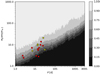 |
Fig. 3 Global HADES detection map. The color scale expresses the global detection function, p. The red circles mark the position in the parameter space of the confirmed HADES planets (see Fig. 1), while the yellow circles indicate the additional candidates presented in this study (see Table 2). |
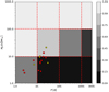 |
Fig. 4 Averaged HADES detection map. The color scale expresses the global detection function, p, averaged over the intervals Δ(P, M) defined for the computation of the occurrence rates. The red circles mark the positions in the parameter space of the confirmed HADES planets (see Fig. 1), while the yellow circles indicate the additional candidates presented in this study (see Table 2). |
5.1 HZ occurrence rates
An aspect of great interest in the studies of occurrence rates of low-mass planets is the parameter η⊕, the frequency of low-mass habitable planets, that is, planets with masses mp sin i < 10 M⊕ orbiting at a distance from their host star that allows the presence of liquid water on their surface, in other words, within the so-called habitable zone (HZ, Kasting et al. 1993). We compute the HZ limits following the recipe from Kopparapu et al. (2013b), defining a conservative and an optimistic HZ: the conservative HZ is computed adopting the runaway greenhouse and maximum greenhouse coefficients for its inner and outer limits respectively; the optimistic limits of the HZ, aHZ,in and aHZ,out are instead computed with the recent Venus and early Mars coefficients, respectively (Kopparapu et al. 2013a).
Thus far no planet has been confirmed inside the conservative or optimistic HZs of any HADES target (see Fig. 1). However, we can still compute an upper limit of the frequency of habitable planets. Therefore, we generated an additional detection map of the HADES samples as a function of the minimum mass and of the position inside the HZ: this was done for each target by computing the detectability functions pi as in Sect. 4, but the posterior of the period Ptest was first converted into the posterior of semi-major axis atest and then the semi-major axis was converted in HZ logarithmic scale, atest,HZ:
 (15)
(15)
this way atest,HZ = 0 corresponds to the inner edge of the optimistic HZ, atest,HZ, and atest,HZ = 1 to the outer edge, atest,out This conversion allow us to compare the HZs of different stars, which are located at different intervals of the semi-major axis parameter space.
For each star, we computed  over a 100 × 100 logarithmic grid in the [aHZ, M] parameter space, where the range of the converted semi-major axis, aHZ, was [0,1], and the minimum-mass range was [1,100] M⊕. We then computed the global detection function inside the HZ pHZ following Eq. (4). The result is shown in Fig. 7.
From the detection function pHZ, taking into account only the confirmed planets none of which were detected inside the HZ (i.e. kHZ = 0), we were able to use Eq. (14) to compute the upper limits of the occurrence rate focc,HZ = η⊕ as before: for low-mass planets, mp sin i < 10 M⊕, we obtained an upper limit focc,HZ = η⊕ < 0.23. Moreover, we also computed the occurrence rate of higher-mass planets inside the HZ, that is 10 M⊕ < mp sin i < 100 M⊕, obtaining focc,HZ < 0.03.
Moreover, we detected one potential planetary signal located inside the optimistic HZ of its host star: GJ 399 32.9 d candidate is located inside the HZ close to its inner edge. However, this signal is slightly less significant than the threshold we adopted in Sect. 3.2.1 (ΔBIC = 9.5), and is therefore not considered as a planetary candidate in Sect. 3.4 and Table 2. Nonetheless, we chose to take it into account to compute a second estimate of η⊕. Taking this candidate into account, the occurrence rate for mp sin i < 10 M⊕ increases to  .
.
Occurrence rates of planets in the HADES sample.
5.2 Long-period companions occurrence rates
It is more difficult to estimate the occurrence rates of long-period planets, that is those with P ≳ 3000 d, which we were only able to detect as linear RV trends due to the relatively short time-span of our survey. As we detected some linear trends with no apparent stellar origin, as discussed in Sect. 3.5, we discuss a few approximations and caveats adopted in order to try and estimate the occurrence rates of the associated long-period planets. It should be noted that the uncertainties on such estimates are intrinsically very large, and very strong approximations are required, but the results could provide interesting information about the little-known field of long-period planets around M dwarfs, and therefore we proceeded anyway.
First we needed to estimate the planetary parameters from the information we can obtain from the linear trends: were able to compute an estimate of the minimum orbital period Pmin in the approximation of a circular orbit as four times the timespan of the observations Pmin ≳ 4 Ts7; similarly, we computed the minimum RV semi-amplitude Kmin as the total RV variation during the observations, that is Kmin ≳ Ts d. From Pmin and Kmin, the corresponding ‘minimum’ minimum mass (mp sin i)min can be derived. The resulting minimum planetary parameters are listed in Table 7. In the case of the GJ 3997 quadratic trend, we were able to approximate the minimum RV amplitude Kmin as the difference between the maximum and minimum RV values of the quadratic curve during the time-span of the observations, Kmin = RVmax − RVmin, while we computed the period as a function of the quadratic acceleration, q, as  (Kipping et al. 2011).
Another obstacle to overcome is the computation of the detection efficiency for such long-period signals, which cannot be computed following our standard recipe described in Sect. 3.1 because the emcee test-planet approach cannot be robustly applied to periods much longer than the time-span of the time-series. We decided to assess the detection efficiency of the HADES time-series towards long-period signals, that is P ≳ 3000 d, by computing for each detected long-term trend d the number of time-series in which that trend could be detected with a significance larger than >3σ, that is in which d > 3 σd,i, where σd,i is the measured uncertainty of the acceleration term in the best-fit MCMC solution of the ith time-series. The resulting numbers of sensitive time-series for each trend, nt, are listed in the last column of Table 7. The mean value of nt can be then used along with the number of significant trends, kt, to estimate the occurrence rate focc,t from Eq. (14).
As discussed in Sect. 3.5, we conducted a few tests to ascertain whether or not the measured RV trends could be caused by other phenomena such as magnetic cycles or stellar companions. A more in-depth analysis is beyond the scope of the present work, but we can compute some preliminary estimates of the occurrence rates, assuming that all the observed trends are due to actual long-period planetary companions. The resulting frequency of planets with P ≳ 3000 d and mp sin i ≳ 10 M⊕ is therefore  As the minimum masses listed in Table 7 are quite diverse, and cover two different intervals of mass defined in the analysis of the short-period planet occurrence rates (Fig. 4), we were able to divide the trend sample into two subsamples with minimum masses larger and smaller than 100 M⊕. Computing the occurrence rates for these two subsamples separately, we obtain
  for long-period planets with mp sin i > 100 M⊕, and
  for long-period planets with 10 M⊕ < mp sin i < 100 M⊕.
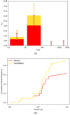 |
Fig. 5 Planetary occurrence rate focc as a function of the orbital period, with the corresponding 1σ uncertainties (top panel). The median cumulative planet frequency is shown in the lower panel. The red and yellow distributions correspond to the occurrence rates derived from the confirmed-only, kp, and confirmed+candidates planets, kc, respectively. |
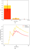 |
Fig. 6 Planetary occurrence rate focc as a function of the minimum mass, with the corresponding 1 σ uncertainties (top panel). The median cumulative planet frequency is shown in the lower panel. The red and yellow distributions correspond to the occurrence rates derived from the confirmed-only, kp, and confirmed + candidates planets, kc, respectively. |
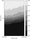 |
Fig. 7 Habitable zone HADES detection map, derived as described in Sect. 5.1. The colour scale expresses the detection function, as in Fig. 3. |
Long-period candidate planetary signals assumed from the modelled linear RV trends.
6 Discussion
We now discuss the main features of our results concerning the sensitivity of the HADES survey and the occurrence rates of extrasolar planets around early M dwarfs, comparing them with previous studies on the planetary population of M dwarfs and earlier-type stars, both from RV surveys and photometric surveys such as Kepler. It is worth noting that the comparison between RV and photometric surveys is far from trivial, because it strongly depends on the mass—radius relations which are still largely unknown, in particular for small low-mass planets.
6.1 Comparison with other RV surveys
We can see in Fig. 6a that the occurrence rate of planets around early-M dwarfs increases strongly towards lower masses. If we take into account only the confirmed HADES planets (red distribution), the occurrence rate rises from  , for 10 M⊕ < mp sin i < 100 M⊕, to
  , for 1 M⊕ < mp sin i < l0 M⊕. This confirms the expected behaviour that was previously observed in other surveys of later-M dwarfs (Bonfils et al. 2013; Tuomi et al. 2014). The occurrence rate as a function of the orbital period, as shown in Fig. 5a, instead appears to peak at intermediate periods, with the highest value
  , for 10 d< P < 100 d, which is roughly 2σ higher than the value for P < 10 d,
 . These behaviours are accentuated if we also take into account the additional planetary candidates presented in Sect. 3.4 (yellow distributions in Fig. 5). It is worth noting that this is due to the fact that most of the detected planets and candidates in the HADES samples are gathered around periods of a few tens of days and masses of around 10 M⊕ (Fig. 3), even if the detection probability in that region of the parameter space is quite low, p ≃ 50%. This confirms what was previously reported by Tuomi et al. (2014) in their study of UVES and HARPS RV data, and could also correspond to the overabundance of transiting planets with similar periods and radii smaller than 3 R⊕ observed around Kepler M dwarfs: Dressing & Charbonneau (2015) observed a higher occurrence rate of planets with 10 d< P < 50 d with respect to those with P < 10 d, albeit not as significant as that observed in our sample. Moreover, it is worth noting that the cumulative planet distribution as a function of the minimum mass (Fig. 6b) suggests that the planet-mass distribution might show a valley between 3 and 5 M⊕, where the cumulative frequency decreases steadily due to the increasing sensitivity of the survey. However, due to the limited number of detected planets, the uncertainties on the fine details of the planet distributions are still quite large.
As shown in Table 5, we derive an occurrence rate of low-mass (1 M⊕ < mp sin i < 10 M⊕) short-period (1 d < P < 10 d) planets around early-M dwarfs of  , which is lower (≃2σ) than the frequency derived by Bonfils et al. (2013) for later-M dwarfs,
  . This could indicate that early-and late-type M dwarfs have different populations of low-mass short-period planets. Even taking into account all the candidate planets that we discussed in Sect. 3.4, our estimate of focc is still ≃1.5σ lower than that of Bonfils et al. (2013) (Table 6), which could still be evidence of this phenomenon. On the other hand, the same effect does not appear to be present for periods 10 d < P < 100 d, where our estimate of
  is perfectly compatible with the value obtained for later-M dwarfs, or even higher if all the candidates planets were confirmed (although still within the 1σ uncertainty of the value obtained by Bonfils et al. (2013)
  . It is worth noting that we find very large upper limits (>1) for low-mass planets with periods larger than 100 d, and this is in line with previous results (Tuomi et al. 2014): this is due to the low sensitivity of RV surveys to low-mass planets at these periods. However, it is interesting to notice that, due to this lack of observational constraints, low-mass planets at intermediate periods (100 d < P < 1000 d) could be very abundant, even if only four such planets have been detected between both RV and transit surveys to date8.
Sabotta et al. (2021), analysing a subsample of the CARMENES survey, found slightly higher occurrence rates than Bonfils et al. (2013), although compatible within 1σ with their results in all period and minimum-mass bins in which both surveys had detected planets. It is interesting to notice that Sabotta et al. (2021) found a relatively high frequency of giant planets (100 M⊕ < mp sin i < 1000 M⊕) with periods up to 1000 d,  , which is somewhat larger than our upper limit of focc < 0.02. However, as they mention in their work, this could be explained by the fact that the results of Sabotta et al. (2021) could be biased by the selection criteria of the analysed subsample. For intermediate masses (10 M⊕ < mp sin i < 100 M⊕), Sabotta et al. (2021) found increasing planetary frequencies towards longer periods up to 1000 d, which appears to be in contrast with our occurrence rates that peaks at intermediate periods (see Table 5); it is nevertheless worth noticing that our estimate of the frequencies of long-period planets (see Sect. 6.3) is quite large, which could confirm the increasing trend observed by Sabotta et al. (2021). Looking at the frequency of low-mass short-period planets, Sabotta et al. (2021) found
  , which is higher than both our estimates and that from the HARPS M-dwarf survey (Bonfils et al. 2013). This again could be explained by the difference in spectral type between the three samples, as the sub-sample analysed by Sabotta et al. (2021) includes later-M dwarfs, which are not observed by the other surveys. Moreover, considering stars with masses higher and lower than 0.34 M⊕ separately, the CARMENES occurrence rates become focc < 0.22 and
  , respectively: while the former value is compatible with our estimate of
  , the latter is significantly higher (>3σ) than our value, which again suggests that the frequency of small-mass planets strongly increases with later spectral types.
6.2 Comparison with transiting planets
Comparing with the frequency of small planets around Kepler M dwarfs, it is evident that our derived occurrence rates for early-M dwarfs are much lower than the average per star of 2.2 ± 0.3 planets with 1 R⊕ < Rp < 4 R⊕ and 1.5 d< P < 180 d derived by Gaidos et al. (2016).9 However, Hardegree-Ullman et al. (2019) found that the number of planets per star with orbital periods shorter than 10 d for Kepler mid-M dwarfs decreases from M5 V to M3 V stars. Assuming this effect also applies to intermediate-period planets, this could mitigate the difference between our RV-based results and Kepler occurrence rates, as the sample analysed by Gaidos et al. (2016) includes many later-type M dwarfs which are not included in our survey. The results from Hardegree-Ullman et al. (2019) also confirm the discrepancy we observed between our early-M sample and the later-type survey of Bonfils et al. (2013).
Moreover, Muirhead et al. (2015) found that  of Kepler early-M dwarfs host compact multi-planets systems with orbital periods lower than 10 d: while this frequency could be consistent with the frequency of short-period low-mass planetary systems we derive from our survey, namely
  , when also taking into account the candidate planets10, we found only one system hosting two short-period planets (GJ 3998 Affer et al. 2016), while all other detected systems contained only a single planet. This apparent incompatibility could be mitigated by selection effects, because many multiple systems discovered by Kepler are composed of small 1−2 R⊕ planets, which could easily fall below our
  M⊕ detection threshold for planets with periods shorter than 10 d (Marcy et al. 2014). Moreover, many Kepler multi-planet systems host planets with very short periods below 2 d, which are inherently difficult to detect in ground-based surveys because of daily sampling limitations. Another possible explanation of the discrepancy between the number of multi-planet systems found in our RV survey and the statistics of Kepler planets could be found in the metallicity of our sample: recent studies (e.g. Anderson et al. 2021) found evidence that Kepler compact multiple planetary systems are hosted by M dwarfs that are statistically more metal-poor than the general population of systems with no detected transiting planets. This is coherent with the observed behaviour of Sun-like stars, which show increasing frequencies of compact multiple systems for metallicities [Fe/H] < −0.3 (Brewer et al. 2018). The complete HADES sample has a mean [Fe/H] = −0.13, and the planet-hosting subsample has a similar mean metallicity of [Fe/H] = −0.15 (see Fig. 8): as the M dwarfs in our sample are relatively metal-rich compared to the bulk of compact-system-hosting Kepler stars, this could explain the scarcity of multiple planetary systems detected by our survey. This could also be in line with the results from the analysis in Maldonado et al. (2020), which showed that there might be an anti-correlation between the frequency of low-mass planets and stellar metallicity.
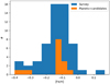 |
Fig. 8 Distribution of stellar metallicities for the HADES samples and for the subsample of planet-hosting stars (including also planetary candidates from Sect. 3.4). |
6.3 Long-period and giant planets
From our analysis of long-term trends, in the assumption that all the trends listed in Table 3 are in fact of planetary origin, we can estimate the frequency of long-period (P > 3 × 10³ d) planets. We estimate that, for intermediate masses (10 M⊕ < mp sin i < 100 M⊕), such planets could be quite abundant around early-M dwarfs,  , with a much higher frequency than the estimate for the same masses and periods 103 d < P < 3 × 10³ d (Table 6). This result could be confirmed by the similar occurrence rate focc ≃ 0.20 computed by Tuomi et al. (2014) for planets with periods longer than 1000 d, even if their survey suffered from the same limitations discussed in Sect. 5.2 due to the similar time-span of the observations. Moreover, this would confirm the trend observed by Sabotta et al. (2021), who measured increasing intermediate-mass planet frequencies at increasing periods. Therefore, our survey confirms the scarcity of giant planets (100 M⊕ < mp sin i < 1000 M⊕) at short-to-intermediate periods around M dwarfs, setting an upper limit to their occurrence focc < 0.02 for periods P < 3000 d (Table 5). This is consistent with the behaviour observed for later-M dwarfs by Bonfils et al. (2013), who estimated the frequency of giant planets of periods up to 1000 d to be focc ≃ 0.02, even if their sample did in fact contain two such planets. Moreover, having detected two very-long-period giant planets (GJ 849 b and GJ 832b), they estimated the frequency of giant planets with periods 103 d < P < 104 d to be
  . Even if the time-span of our survey did not allow for the detection of such long-period planets, this result is perfectly compatible with our estimate of the frequency of long-period giant planets derived from the observed RV trends
  (Sect. 5.2). However, the occurrence rate we derive is larger (≃2σ) than the estimated frequency of Jupiter-like planets around M dwarfs computed combining RV and microlensing surveys,
  (Clanton & Gaudi 2014). Moreover, it is worth noting that the focc,t we derived is very close to the recent results by Wittenmyer et al. (2020), who derived the frequency of cool Jupiters to be
  from an RV survey of FGK stars. This could suggest that the frequency of long-period giant planets does not vary as strongly as the frequency of low-mass planets from Solar-type stars to M dwarfs.
Comparing Fig. 1 and Table 2 to Table 3, it is interesting to notice that, apart from GJ 15A, none of our stars hosting short-period low-mass planets show a long-period trend compatible with the presence of an outer planetary companion. This appears to be in contrast with theoretical models, as Izidoro et al. (2015) predicted that systems with only one low-mass planet with orbital period shorter than 100 d should also harbour a Jupiter-like planet on a more distant orbit: otherwise both in situ formation and inward migration models predict that super-Earth and warm Neptunes should form in rich systems hosting many close-in planets. However, of all of our detected planets and candidates, only one system appears to host more than a single close-in planet (GJ 3998), and, as previously mentioned, the other systems do not show any evidence of the expected outer massive companions.
6.4 Habitable planets
The HADES program has not been able to confirm the presence of any planet in the HZ so far, and therefore even if the detection function was generally low for low-mass planets in the HZ (Fig. 7), we derived an upper limit to the frequency of habitable planets around early-M dwarfs of η⊕ < 0.23 (see Sect. 5.1). Bonfils et al. (2013) estimated a higher frequency of habitable planets around M dwarfs  . However, this value takes into account the presence of the habitable planet GJ 581 d, which was later discarded as an artifact of stellar activity (Baluev 2013; Robertson et al. 2014). Therefore, recomputing their value of η⊕ considering only the other habitable planet detected in their survey, the obtained value is lower η⊕ ≃ 0.20, which is much closer to the value derived from our analysis of the HADES survey. Moreover, Tuomi et al. (2014) found a similar value of
  considering planets with masses 3 M⊕ < mp sin i < 10 M⊕, which is compatible within 1σ with our estimate. The upper limit we derived, η⊕ < 0.23, could still allow a higher number of low-mass planets in the HZ of early-M dwarfs compared to G-type stars, for which the fraction of Earth-like planets is estimated to be η⊕ ≃ 0.10 (Perryman 2018). Instead, if we consider the weak candidate planet detected in this analysis orbiting in the outer rim of the HZ of its host star, our estimate of η⊕ increases to
  , which would be compatible with the previous estimates from RV M-dwarf surveys, and confirm the abundance of habitable planets around low-mass stars compared to Solar-type stars.
7 Conclusions
We presented the statistical analysis of the spectroscopic observations of a magnitude-limited sample of nearby early-M dwarfs observed within the HADES programme. The sample is composed of 56 targets, each with an average of 77 high-precision RVs. We analysed all of the time-series in the sample with a uniform Bayesian technique in order to obtain consistent and unbiased estimates of the detection limits and planetary occurrence rates. Moreover, we applied GP regression to refine the planetary parameters and improve the detection efficiency around the most observed and active targets in the survey.
The sample includes ten published planetary systems discovered and characterised as part of the HADES programme, and in this work we present five new planetary candidates. Moreover, we discuss eight RV long-term trends that could be produced by long-period planetary companions. The new candidates will be further analysed and discussed in future focused publications, two of which are in preparation and soon to be submitted (González Hernández et al. on GJ 21 and Affer et al. on GJ 3822). The other candidates, and in particular the weak HZ candidate discussed in Sect. 5.1, will need additional RV observations to confirm or disprove their planetary nature. Similarly, an in-depth analysis of the long-term trends will be the focus of a future dedicated work, as a survey focused on the characterization of late-type systems hosting long-period planets is currently being carried out within the GAPS programme (Barbato et al. 2020).
We confirm that giant planets (100 M⊕ < mp sin i < 1000 M⊕) are very rare around M dwarfs at short-to-intermediate periods (P < 3000 d), focc < 0.02. On the other hand, low-mass planets (1 M⊕ < mp sin i < 10 M⊕) appear to be common, with frequencies varying between  for short periods (1 d < P < 10 d) to
  for longer periods (10 d < P < 100 d). While high compared to Solar-type stars, these frequencies appear to be lower than for later-M systems, therefore confirming the strong dependence of planetary occurrence rates on stellar mass. It is worth noting that early- and late-M dwarfs have very different internal structures, as the latter are fully convective, and this affects the efficiency of tidal interaction between a star and a close-by planet (Barker 2020), which could explain the significant difference in planetary occurrence rates between early- and late-M dwarfs. We also estimated the frequency of habitable planets around early-M dwarfs, finding an upper limit of η⊕ < 0.23, which suggests that the frequency of Earth-like planets around such stars is as high as if not higher than around Solar-type stars.
Finally, it is worth noting how the current number of HADES close-in planets (11–16) is incompatible with the prediction of 3.8 ± 1.9 detections (Perger et al. 2017a) based on previous M-dwarf planet population models. This highlights the importance of long-term high-precision surveys focused on narrow intervals of stellar masses in improving our knowledge of planetary populations, and therefore formation mechanisms, through different classes of stellar hosts.
Acknowledgements
M.Pi., A.P., A.M., and A.S. acknowledge partial contribution from the agreement ASI-INAF n.2018-16-HH.0. M.Pi. acknowledges partial contribution from OB.FU. 1.05.02.85.13 “Planetary Systems At Early Ages (PLATEA)”. J.M., and G.M. acknowledge support from the accordo attua-tivo ASI-INAF n.2021-5-HH.0 “Partecipazione italiana alla fase B2/C della missione Ariel”. E.G.A. acknowledge support from the Spanish Ministery for Science, Innovation, and Universities through projects AYA-2016-79425-C3-1/2/3-P, AYA2015-69350-C3-2-P, ESP2017-87676-C5-2-R, ESP2017-87143-R. The Centro de Astrobiología (CAB, CSIC-INTA) is a Center of Excellence “Maria de Maeztu”. M.D. acknowledges financial support from the FP7-SPACE Project ETAEARTH (GA no. 313014). P.G. gratefully acknowledges support from the Italian Space Agency (ASI) under contract 2018-24-HH.0. M.Pe. and I.R. acknowledge support from the Spanish Ministry of Science and Innovation and the European Regional Development Fund through grant PGC2018-098153-B- C33, as well as the support of the Generalitat de Catalunya/CERCA programme. J.I.G.H. acknowledges financial support from Spanish Ministry of Science and Innovation (MICINN) under the 2013 Ramón y Cajal program RYC-2013- 14875. B.T.P. acknowledges Fundación La Caixa for the financial support received in the form of a Ph.D. contract. A.S.M. acknowledges financial support from the Spanish MICINN under the 2019 Juan de la Cierva Programme. B.T.P., A.S.M., J.I.G.H. and R.R. acknowledge financial support from the Spanish MICINN project PID2020-117493GB-I00, and from the Government of the Canary Islands project ProID2020010129. The HARPS-N Project is a collaboration between the Astronomical Observatory of the Geneva University (lead), the CfA in Cambridge, the Universities of St. Andrews and Edinburgh, the Queen’ss University of Belfast, and the TNG-INAF Observatory. This work has made use of data from the European Space Agency (ESA) mission Gaia (https://www.cosmos.esa.int/gaia), processed by the Gaia Data Processing and Analysis Consortium (DPAC, https://www.cosmos.esa.int/web/gaia/dpac/consortium). Funding for the DPAC has been provided by national institutions, in particular the institutions participating in the Gaia Multilateral Agreement. We also thank the anonymous referee for the insightful review.
Appendix A MCMC analysis: Planetary parameters, GP hyper-parameters, and adopted priors
We adopted uninformative priors for all the parameters and hyper-parameters in our MCMC models. This was done for consistency across the statistical analysis, and to avoid adulterating the computed detection function by adopting incorrect informative priors. For most of the RV model parameters and GP hyper-parameters we adopted a uniform prior, except for the correlation decay timescale, λ, for which we adopted a uniform prior in logarithmic scale to avoid oversampling the long scales, as λ can be of the order of tens or hundreds of days and more, depending on the activity level of the target. When an eccentric Keplerian signal was included in the model, instead of fitting separately ej and ωj, we use the auxiliary parameters  · cos ωj and
  · sin ωj to reduce the covariance between ej and ωj, especially for low eccentricity value. Moreover, when the eccentricity was consistent with ej = 0 we adopted a circular model, fixing ej = ωj = 0, to reduce the number of parameters and the computational weight of the analysis.
The analysis of GJ 15A required some different priors for the RV model because, as discussed in Pinamonti et al. (2018), the complete orbital solution was obtained by a combination of HIRES + HARPS-N data, and was not recoverable from HARPS-N data only. For this reason, we applied Gaussian priors to the GP hyper-parameters, to the semi-amplitude and period of the inner planets GJ 15A b, and to the acceleration coefficient d, which as discussed in Sect. 3.4 corresponds to the RV variations caused by the outer planet GJ 15A c over the timespan of the HARPS-N observations.
Finally, particular care was required for the three parameters of the test-planet RV model, whose prior could directly impact the resulting  function. For the orbital period Ptest we adopted a uniform prior in logarithmic scale over the interval log
  , choosing the upper limit to be roughly twice the average timespan of the observations. The prior of RV amplitude Ktest required a particularly large prior to avoid constraining the derived minimum-mass values over all the explored orbital period values: for this reason we adopted a very broad logarithmic uniform prior log
  , with an upper limit sufficiently larger than the maximum r.m.s. of the HADES time-series (see Table 1). Lastly, to fit the reference time of the test-planet orbit, T0,test, we defined the auxiliary parameter tp,test = Tc/Ptest, with Tc the time of inferior conjunction: tp,test could be thus defined over a uniform prior
  , avoiding the multi-modal distribution of Tc, which could greatly impact the efficiency of emcee (Foreman-Mackey et al. 2013).
Moreover, in Fig. A.1 is shown the detection function map of GJ399, with marked the position of the 32.9 signal identified in the RV time-series which, as discussed in Sect. 5.1, is just below the acceptance threshold ΔBIC = 10: it is worth noticing that the weak-candidate signal mass, Mp sin i = 7.0 M⊕, is just below the  M⊕ detection threshold for periods in [20,40] d. This confirms the good correspondence between the adopted planetary acceptance criterion (Sect. 3.2.1) and the MCMC-derived detectability function (Sect. 3.2).
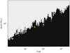 |
Fig. A.1 Detection function map of the RV time-series of GJ 399 (as in Fig. 2). The yellow circle shows the position of the 32.9 d weak candidate signal. |
Appendix B New planetary candidates
In Fig. B.1 to B.5 the relevant plots describing the planetary candidates detected in this analysis, as discussed in Sect. 3.4, are shown. The periodic signals in the RV data are shown via the Generalized Lomb Scargle periodogram analysis (GLS, Zechmeister & Kürster 2009) of the RV time-series, after all stellar signals and the Base Model have been removed.
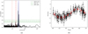 |
Fig. B.1 Planetary candidate in the GJ 21 system. a) GLS periodogram of the RV time-series after subtracting the Base Model and the GP activity signal. The vertical blue dashed line marks the orbital period of the candidate, while the vertical red dot-dashed and dotted lines show the stellar rotation period and its first harmonic, respectively. b) Phase-folded for the RV curve of the planetary candidate. The red solid line represents the best-fit Keplerian model, while the red circles indicates the binned RVs with the corresponding rms. |
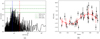 |
Fig. B.2 Planetary candidate in the GJ 1074 system. a) GLS periodogram of the RV time-series after subtracting the Base Model. The vertical blue dashed line marks the orbital period of the candidate, while the vertical red dot-dashed line shows the stellar rotation period as derived by Suárez Μascareño et al. (2018). b) Phase-folded for the RV curve of the planetary candidate. The red solid line represents the best-fit Keplerian model, while the red circles indicates the binned RVs with the corresponding rms. |
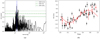 |
Fig. B.3 Planetary candidate in the GJ 9404 system. a) GLS periodogram of the RV time-series after subtracting the Base Model. The vertical blue dashed line marks the orbital period of the candidate. b) Phase-folded for the RV curve of the planetary candidate. The red solid line represents the best-fit Keplerian model, while the red circles indicates the binned RVs with the corresponding rms. |
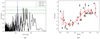 |
Fig. B.4 Planetary candidate in the GJ 548A system. a) GLS periodogram of the RV time-series after subtracting the Base Model. The vertical blue dashed line marks the orbital period of the candidate. b) Phase-folded for the RV curve of the planetary candidate. The red solid line represents the best-fit Keplerian model, while the red circles indicates the binned RVs with the corresponding rms. |
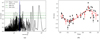 |
Fig. B.5 Planetary candidate in the GJ 3822 system. a) GLS periodogram of the RV time-series after subtracting the Base Model. The vertical blue dashed line marks the orbital period of the candidate. b) Phase-folded for the RV curve of the planetary candidate. The red solid line represents the best-fit Keplerian model, while the red circles indicates the binned RVs with the corresponding rms. |
Appendix C MCMC analysis: best-fit RV models
The best-fit models of all the HADES targets fitted in this analysis are summarised in Table C.1. The best-fit model components are abbreviated as follow: GP best-fit model includes GP regression as described in Sect. 3.3; BM Base Model from Eq. 6; Quad quadratic component added to the Base Model as in Eq. 13; Kpl(ecc) full Keplerian component from Eq. 7; Kpl(circ) circular Keplerian component with e = ω = 0 in Eq. 7; Act stellar activity RV signal, modelled as a sine wave as discussed in Sect. 3.3..
Best-fit RV models of the targets of the survey.
References
- Adibekyan, V. Z., Sousa, S. G., Santos, N. C., et al. 2012, A&A, 545, A32 [NASA ADS] [CrossRef] [EDP Sciences] [Google Scholar]
- Affer, L., Micela, G., Damasso, M., et al. 2016, A&A, 593, A117 [NASA ADS] [CrossRef] [EDP Sciences] [Google Scholar]
- Affer, L., Damasso, M., Micela, G., et al. 2019, A&A, 622, A193 [NASA ADS] [CrossRef] [EDP Sciences] [Google Scholar]
- Ambikasaran, S., Foreman-Mackey, D., Greengard, L., Hogg, D. W., & O'Neil, M. 2015, IEEE Trans. Pattern Anal. Mach. Intell., 38, 252 [Google Scholar]
- Anderson, S. G., Dittmann, J. A., Ballard, S., & Bedell, M. 2021, AJ, 161, 203 [NASA ADS] [CrossRef] [Google Scholar]
- Anglada-Escudé, G., & Butler, R. P. 2012, ApJS, 200, 15 [Google Scholar]
- Anglada-Escudé, G., Tuomi, M., Gerlach, E., et al. 2013, A&A, 556, A126 [NASA ADS] [CrossRef] [EDP Sciences] [Google Scholar]
- Anglada-Escudé, G., Tuomi, M., Arriagada, P., et al. 2016, ApJ, 830, 74 [CrossRef] [Google Scholar]
- Astudillo-Defru, N., Forveille, T., Bonfils, X., et al. 2017, A&A, 602, A88 [NASA ADS] [CrossRef] [EDP Sciences] [Google Scholar]
- Baluev, R. V. 2013, MNRAS, 429, 2052 [Google Scholar]
- Barbato, D., Pinamonti, M., Sozzetti, A., et al. 2020, A&A, 641, A68 [EDP Sciences] [Google Scholar]
- Barker, A. J. 2020, MNRAS, 498, 2270 [Google Scholar]
- Bonfils, X., Mayor, M., Delfosse, X., et al. 2007, A&A, 474, 293 [NASA ADS] [CrossRef] [EDP Sciences] [Google Scholar]
- Bonfils, X., Delfosse, X., Udry, S., et al. 2013, A&A, 549, A109 [NASA ADS] [CrossRef] [EDP Sciences] [Google Scholar]
- Brewer, J. M., Wang, S., Fischer, D. A., & Foreman-Mackey, D. 2018, ApJ, 867, L3 [NASA ADS] [CrossRef] [Google Scholar]
- Clanton, C., & Gaudi, B. S. 2014, ApJ, 791, 91 [NASA ADS] [CrossRef] [Google Scholar]
- Covino, E., Esposito, M., Barbieri, M., et al. 2013, A&A, 554, A28 [NASA ADS] [CrossRef] [EDP Sciences] [Google Scholar]
- Cumming, A., & Dragomir, D. 2010, MNRAS, 401, 1029 [NASA ADS] [CrossRef] [Google Scholar]
- Cumming, A., Butler, R. P., Marcy, G. W., et al. 2008, PASP, 120, 531 [CrossRef] [Google Scholar]
- Damasso, M., Pinamonti, M., Scandariato, G., & Sozzetti, A. 2019, MNRAS, 489, 2555 [NASA ADS] [CrossRef] [Google Scholar]
- Dekker, H., D'Odorico, S., Kaufer, A., Delabre, B., & Kotzlowski, H. 2000, in Proc. SPIE, 4008, Optical and IR Telescope Instrumentation and Detectors, eds. M. Iye, & A. F. Moorwood, 534 [NASA ADS] [CrossRef] [Google Scholar]
- Desidera, S., Sozzetti, A., Bonomo, A. S., et al. 2013, A&A, 554, A29 [NASA ADS] [CrossRef] [EDP Sciences] [Google Scholar]
- Dressing, C. D., & Charbonneau, D. 2013, ApJ, 767, 95 [Google Scholar]
- Dressing, C. D., & Charbonneau, D. 2015, ApJ, 807, 45 [Google Scholar]
- Dumusque, X., Lovis, C., Udry, S., & Santos, N. C. 2011, in IAU Symposium, 276, The Astrophysics of Planetary Systems: Formation, Structure, and Dynamical Evolution, eds. A. Sozzetti, M. G. Lattanzi, & A. P. Boss, 530 [NASA ADS] [Google Scholar]
- Dumusque, X., Glenday, A., Phillips, D. F., et al. 2015, ApJ, 814, L21 [Google Scholar]
- Eastman, J., Gaudi, B. S., & Agol, E. 2013, PASP, 125, 83 [Google Scholar]
- Endl, M., Kürster, M., Els, S., et al. 2002, A&A, 392, 671 [CrossRef] [EDP Sciences] [Google Scholar]
- Endl, M., Cochran, W. D., Tull, R. G., & MacQueen, P. J. 2003, AJ, 126, 3099 [Google Scholar]
- Endl, M., Cochran, W. D., Kürster, M., et al. 2006, ApJ, 649, 436 [Google Scholar]
- Feng, F., Butler, R. P., Shectman, S. A., et al. 2020, ApJS, 246, 11 [Google Scholar]
- Foreman-Mackey, D., Hogg, D. W., Lang, D., & Goodman, J. 2013, PASP, 125, 306 [Google Scholar]
- Gaia Collaboration (Prusti, T., et al.) 2016, A&A, 595, A1 [NASA ADS] [CrossRef] [EDP Sciences] [Google Scholar]
- Gaia Collaboration (Brown, A. G. A., et al.) 2021, A&A, 649, A1 [NASA ADS] [CrossRef] [EDP Sciences] [Google Scholar]
- Gaidos, E., Mann, A. W., Kraus, A. L., & Ireland, M. 2016, MNRAS, 457, 2877 [Google Scholar]
- Giacobbe, P., Benedetto, M., Damasso, M., et al. 2020, MNRAS, 491, 5216 [Google Scholar]
- Giles, H. A. C., Collier Cameron, A., & Haywood, R. D. 2017, MNRAS, 472, 1618 [Google Scholar]
- Gomes da Silva, J., Santos, N. C., Bonfils, X., et al. 2011, A&A, 534, A30 [NASA ADS] [CrossRef] [EDP Sciences] [Google Scholar]
- González-Álvarez, E., Micela, G., Maldonado, J., et al. 2019, A&A, 624, A27 [NASA ADS] [CrossRef] [EDP Sciences] [Google Scholar]
- González-Álvarez, E., Petralia, A., Micela, G., et al. 2021, A&A, 649, A157 [NASA ADS] [CrossRef] [EDP Sciences] [Google Scholar]
- Hardegree-Ullman, K. K., Cushing, M. C., Muirhead, P. S., & Christiansen, J. L. 2019, AJ, 158, 75 [Google Scholar]
- Hawley, S. L., Davenport, J. R. A., Kowalski, A. F., et al. 2014, ApJ, 797, 121 [Google Scholar]
- Ida, S., & Lin, D. N. C. 2005, ApJ, 626, 1045 [NASA ADS] [CrossRef] [Google Scholar]
- Izidoro, A., Raymond, S. N., Morbidelli, A., Hersant, F., & Pierens, A. 2015, ApJ, 800, L22 [Google Scholar]
- Kass, R. E., & Raftery, A. E. 1995, J. Am. Stat. Assoc., 90, 773 [Google Scholar]
- Kasting, J. F., Whitmire, D. P., & Reynolds, R. T. 1993, Icarus, 101, 108 [Google Scholar]
- Kervella, P., Arenou, F., & Thévenin, F. 2022, A&A, 657, A7 [NASA ADS] [CrossRef] [EDP Sciences] [Google Scholar]
- Kipping, D. M., Hartman, J., Bakos, G. Ä., et al. 2011, AJ, 142, 95 [NASA ADS] [CrossRef] [Google Scholar]
- Kopparapu, R. K., Ramirez, R., Kasting, J. F., et al. 2013a, ApJ, 770, 82 [NASA ADS] [CrossRef] [Google Scholar]
- Kopparapu, R. K., Ramirez, R., Kasting, J. F., et al. 2013b, ApJ, 765, 131 [NASA ADS] [CrossRef] [Google Scholar]
- Lépine, S., & Gaidos, E. 2013, Astron. Nachr., 334, 176 [CrossRef] [Google Scholar]
- Lindegren, L., Klioner, S. A., Hernandez, J., et al. 2021, A&A, 649, A2 [NASA ADS] [CrossRef] [EDP Sciences] [Google Scholar]
- Lovis, C., Dumusque, X., Santos, N. C., et al. 2011, ArXiv e-prints [arXiv:1187.5325] [Google Scholar]
- Lovis, C., & Pepe, F. 2007, A&A, 468, 1115 [NASA ADS] [CrossRef] [EDP Sciences] [Google Scholar]
- Luque, R., Nowak, G., Pallé, E., et al. 2018, A&A, 620, A171 [NASA ADS] [CrossRef] [EDP Sciences] [Google Scholar]
- Maldonado, J., Affer, L., Micela, G., et al. 2015, A&A, 577, A132 [NASA ADS] [CrossRef] [EDP Sciences] [Google Scholar]
- Maldonado, J., Scandariato, G., Stelzer, B., et al. 2017, A&A, 598, A27 [NASA ADS] [CrossRef] [EDP Sciences] [Google Scholar]
- Maldonado, J., Micela, G., Baratella, M., et al. 2020, A&A, 644, A68 [EDP Sciences] [Google Scholar]
- Maldonado, J., Petralia, A., Damasso, M., et al. 2021, A&A, 651, A93 [NASA ADS] [CrossRef] [EDP Sciences] [Google Scholar]
- Marcy, G. W., Isaacson, H., Howard, A. W., et al. 2014, ApJS, 210, 20 [NASA ADS] [CrossRef] [Google Scholar]
- Mayor, M., Pepe, F., Queloz, D., et al. 2003, The Messenger, 114, 20 [NASA ADS] [Google Scholar]
- Mordasini, C., Alibert, Y., Benz, W., Klahr, H., & Henning, T. 2012, A&A, 541, A97 [NASA ADS] [CrossRef] [EDP Sciences] [Google Scholar]
- Muirhead, P. S., Mann, A. W., Vanderburg, A., et al. 2015, ApJ, 801, 18 [NASA ADS] [CrossRef] [Google Scholar]
- Newton, E. R., Irwin, J., Charbonneau, D., Berta-Thompson, Z. K., & Dittmann, J. A. 2016, ApJ, 821, L19 [NASA ADS] [CrossRef] [Google Scholar]
- Perger, M., Garcia-Piquer, A., Ribas, I., et al. 2017a, A&A, 598, A26 [NASA ADS] [CrossRef] [EDP Sciences] [Google Scholar]
- Perger, M., Ribas, I., Damasso, M., et al. 2017b, A&A, 608, A63 [NASA ADS] [CrossRef] [EDP Sciences] [Google Scholar]
- Perger, M., Scandariato, G., Ribas, I., et al. 2019, A&A, 624, A123 [NASA ADS] [CrossRef] [EDP Sciences] [Google Scholar]
- Perryman, M. 2018, The Exoplanet Handbook (Cambridge University Press) [Google Scholar]
- Pinamonti, M., Damasso, M., Marzari, F., et al. 2018, A&A, 617, A104 [NASA ADS] [CrossRef] [EDP Sciences] [Google Scholar]
- Pinamonti, M., Sozzetti, A., Giacobbe, P., et al. 2019, A&A, 625, A126 [NASA ADS] [CrossRef] [EDP Sciences] [Google Scholar]
- Poretti, E., Boccato, C., Claudi, R., et al. 2016, Mem. Soc. Astron. Italiana, 87, 141 [NASA ADS] [Google Scholar]
- Reid, I. N., Hawley, S. L., & Gizis, J. E. 1995, AJ, 110, 1838 [Google Scholar]
- Robertson, P., Mahadevan, S., Endl, M., & Roy, A. 2014, Science, 345, 440 [Google Scholar]
- Sabotta, S., Schlecker, M., Chaturvedi, P., et al. 2021, A&A, 653, A114 [NASA ADS] [CrossRef] [EDP Sciences] [Google Scholar]
- Scandariato, G., Maldonado, J., Affer, L., et al. 2017, A&A, 598, A28 [NASA ADS] [CrossRef] [EDP Sciences] [Google Scholar]
- Schwarz, G., et al. 1978, Ann. Stat., 6, 461 [Google Scholar]
- Selsis, F., Kasting, J. F., Levrard, B., et al. 2007, A&A, 476, 1373 [CrossRef] [EDP Sciences] [Google Scholar]
- Sousa, S. G., Santos, N. C., Mayor, M., et al. 2008, A&A, 487, 373 [NASA ADS] [CrossRef] [EDP Sciences] [Google Scholar]
- Sozzetti, A., Bernagozzi, A., Bertolini, E., et al. 2013, in European Physical Journal Web of Conferences, 47, 03006 [NASA ADS] [CrossRef] [EDP Sciences] [Google Scholar]
- Suárez Mascareño, A., Gonzalez Hernandez, J. I., Rebolo, R., et al. 2017, A&A, 605, A92 [NASA ADS] [CrossRef] [EDP Sciences] [Google Scholar]
- Suárez Mascareño, A., Rebolo, R., Gonzalez Hernandez, J. I., et al. 2018, A&A, 612, A89 [NASA ADS] [CrossRef] [EDP Sciences] [Google Scholar]
- Toledo-Padrón, B., Suarez Mascareno, A., Gonzalez Hernandez, J. I., et al. 2021, A&A, 648, A20 [NASA ADS] [CrossRef] [EDP Sciences] [Google Scholar]
- Tuomi, M., Jones, H. R. A., Barnes, J. R., Anglada-Escudé, G., & Jenkins, J. S. 2014, MNRAS, 441, 1545 [Google Scholar]
- Vanderburg, A., Plavchan, P., Johnson, J. A., et al. 2016, MNRAS, 459, 3565 [NASA ADS] [CrossRef] [Google Scholar]
- Wittenmyer, R. A., Wang, S., Horner, J., et al. 2020, MNRAS, 492, 377 [NASA ADS] [CrossRef] [Google Scholar]
- Yang, H., Liu, J., Gao, Q., et al. 2017, ApJ, 849, 36 [NASA ADS] [CrossRef] [Google Scholar]
- Zechmeister, M., & Kürster, M. 2009, A&A, 496, 577 [CrossRef] [EDP Sciences] [Google Scholar]
HARPS-N spectra have a total of 66 échelle orders.
The MCMC-derived detectability function we adopt in this analysis shows good correspondence with the ΔBIC = 10 detection threshold, as shown in Appendix A.
If a significant correlation was found for more than one activity index, we selected for the linear detrending the time-series that presented the strongest correlation.
This is a good approximation over the HARPS-N time-series, as can be seen in Fig. 6 of Pinamonti et al. (2018).
The RV acceleration produced by the stellar binary is computed assuming a circular orbit edge-on and using the measured separation as semi-major axis.
The derivation of nΔ(P,M) assumes a log-uniform distribution of p over the selected parameter-space intervals Δ(P, M).
This can be assumed because the linear trend could cover up to half of the peak-to-trough part of a sinewave, without showing any evident curvature. Therefore, the observed time-span could correspond to no more than one-quarter of the orbital period.
NASA exoplanet archive - 08/04/2021: GJ 180 d P = 106.300 ± 0.129d, mp sin i = 7.56 ± 1.07 M⊕, GJ 229Ac P = 121.995 ± 0.161 d, mp sin i = 7.268 ± 1.256 M⊕ (Feng et al. 2020); GJ 628 d  ,
,  (Astudillo-Defru et al. 2017); GJ 667Cg
  ,
,  (Anglada-Escudé et al. 2013).
Other studies of Kepler M dwarfs, found lower number of planets per star, ~1.5 for 1 R⊕ < Rp < 4 R⊕ and 1. d < P < 10 (Sabotta et al. 2021, and references therein), but these numbers are still much higher than the occurrence rates we derive from the HADES RV sample.
Assuming the empyrical planet mass—radius relationships of Marcy et al. (2014) adopted by Muirhead et al. (2015).
Bonfils et al. (2013) used the definition of HZ from Selsis et al. (2007), while Tuomi et al. (2014) used the same updated definition we adopted in our work (Kopparapu et al. 2013b).
All Tables
Stellar parameters and summary of the observations of the 56 HADES targets analysed in this work.
Long-period candidate planetary signals assumed from the modelled linear RV trends.
All Figures
|
Fig. 1 Overview of the HADES detected planetary systems. The published planets of the sample are shown as red circles: the symbol size is proportional to the minimum planetary mass. The conservative and optimistic limits of the habitable zone of each system (see Sect. 5.1) are shown as thick dark green and light green bands, respectively. |
| In the text | |
|
Fig. 2 Detection function map of the RV time-series of GJ 15 A. The white part corresponds to the area in the period—minimum mass space where additional signals could be detected if present in the data, i.e. pi = 1, while the black region corresponds to the area where the detection probability is negligible, i.e. pi = 0. The red circle marks the position in the parameter space of the planet GJ 15 A b. |
| In the text | |
|
Fig. 3 Global HADES detection map. The color scale expresses the global detection function, p. The red circles mark the position in the parameter space of the confirmed HADES planets (see Fig. 1), while the yellow circles indicate the additional candidates presented in this study (see Table 2). |
| In the text | |
|
Fig. 4 Averaged HADES detection map. The color scale expresses the global detection function, p, averaged over the intervals Δ(P, M) defined for the computation of the occurrence rates. The red circles mark the positions in the parameter space of the confirmed HADES planets (see Fig. 1), while the yellow circles indicate the additional candidates presented in this study (see Table 2). |
| In the text | |
|
Fig. 5 Planetary occurrence rate focc as a function of the orbital period, with the corresponding 1σ uncertainties (top panel). The median cumulative planet frequency is shown in the lower panel. The red and yellow distributions correspond to the occurrence rates derived from the confirmed-only, kp, and confirmed+candidates planets, kc, respectively. |
| In the text | |
|
Fig. 6 Planetary occurrence rate focc as a function of the minimum mass, with the corresponding 1 σ uncertainties (top panel). The median cumulative planet frequency is shown in the lower panel. The red and yellow distributions correspond to the occurrence rates derived from the confirmed-only, kp, and confirmed + candidates planets, kc, respectively. |
| In the text | |
|
Fig. 7 Habitable zone HADES detection map, derived as described in Sect. 5.1. The colour scale expresses the detection function, as in Fig. 3. |
| In the text | |
|
Fig. 8 Distribution of stellar metallicities for the HADES samples and for the subsample of planet-hosting stars (including also planetary candidates from Sect. 3.4). |
| In the text | |
|
Fig. A.1 Detection function map of the RV time-series of GJ 399 (as in Fig. 2). The yellow circle shows the position of the 32.9 d weak candidate signal. |
| In the text | |
|
Fig. B.1 Planetary candidate in the GJ 21 system. a) GLS periodogram of the RV time-series after subtracting the Base Model and the GP activity signal. The vertical blue dashed line marks the orbital period of the candidate, while the vertical red dot-dashed and dotted lines show the stellar rotation period and its first harmonic, respectively. b) Phase-folded for the RV curve of the planetary candidate. The red solid line represents the best-fit Keplerian model, while the red circles indicates the binned RVs with the corresponding rms. |
| In the text | |
|
Fig. B.2 Planetary candidate in the GJ 1074 system. a) GLS periodogram of the RV time-series after subtracting the Base Model. The vertical blue dashed line marks the orbital period of the candidate, while the vertical red dot-dashed line shows the stellar rotation period as derived by Suárez Μascareño et al. (2018). b) Phase-folded for the RV curve of the planetary candidate. The red solid line represents the best-fit Keplerian model, while the red circles indicates the binned RVs with the corresponding rms. |
| In the text | |
|
Fig. B.3 Planetary candidate in the GJ 9404 system. a) GLS periodogram of the RV time-series after subtracting the Base Model. The vertical blue dashed line marks the orbital period of the candidate. b) Phase-folded for the RV curve of the planetary candidate. The red solid line represents the best-fit Keplerian model, while the red circles indicates the binned RVs with the corresponding rms. |
| In the text | |
|
Fig. B.4 Planetary candidate in the GJ 548A system. a) GLS periodogram of the RV time-series after subtracting the Base Model. The vertical blue dashed line marks the orbital period of the candidate. b) Phase-folded for the RV curve of the planetary candidate. The red solid line represents the best-fit Keplerian model, while the red circles indicates the binned RVs with the corresponding rms. |
| In the text | |
|
Fig. B.5 Planetary candidate in the GJ 3822 system. a) GLS periodogram of the RV time-series after subtracting the Base Model. The vertical blue dashed line marks the orbital period of the candidate. b) Phase-folded for the RV curve of the planetary candidate. The red solid line represents the best-fit Keplerian model, while the red circles indicates the binned RVs with the corresponding rms. |
| In the text | |
Current usage metrics show cumulative count of Article Views (full-text article views including HTML views, PDF and ePub downloads, according to the available data) and Abstracts Views on Vision4Press platform.
Data correspond to usage on the plateform after 2015. The current usage metrics is available 48-96 hours after online publication and is updated daily on week days.
Initial download of the metrics may take a while.