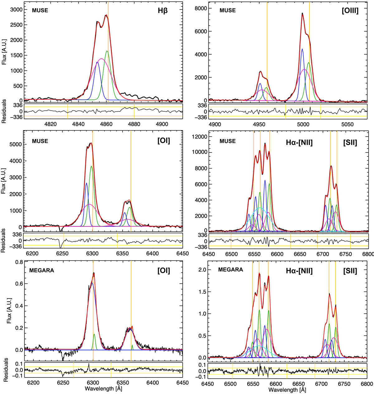
Examples of emission line spectra (black) after stellar subtraction (Sect. 3.2) and their modelling from the central region of both MUSE data (R = 07, i.e. 77 pc) and MEGARA data (R = 09, i.e. 100 pc), as indicated top left. As references, the orange vertical lines give the systemic wavelengths of the emission lines which, are indicated top right. For each panel the modelled line profile (in red) and the components (in different colours) are shown. Specifically, the green, blue, and pink Gaussian curves indicate the primary, secondary, and tertiary components used to model the profiles. The cyan line indicates the broad Hα component from the BLR. Residuals from the fit are shown below each panels; the yellow horizontal lines indicate the ±2.5 ε_c (Sect. 3.3.1) and the vertical yellow lines give the wavelength range considered for calculating ε_fit for each line (Sect. 3.3.1). The high residuals redwards of Hβ cannot be fitted with a BLR component (the velocities and widths would be inconsistent with those of the broad Hα component), and are likely due to some residuals from stellar subtraction (Sect. 3.2).