| Issue |
A&A
Volume 664, August 2022
|
|
|---|---|---|
| Article Number | A89 | |
| Number of page(s) | 13 | |
| Section | Interstellar and circumstellar matter | |
| DOI | https://doi.org/10.1051/0004-6361/202142431 | |
| Published online | 11 August 2022 | |
Supernova remnant G46.8–0.3: A new case of interaction with molecular material
1
Instituto de Astronomía y Física del Espacio (IAFE, CONICET – UBA)
CC 67, Suc. 28,
1428
Buenos Aires, Argentina
e-mail: This email address is being protected from spambots. You need JavaScript enabled to view it.
2
Universidad Nacional del Sur (UNS),
Av. L. N. Alem 1253,
B8000CPB –
Bahía Blanca, Argentina
Received:
13
October
2021
Accepted:
8
March
2022
Abstract
Although the Galactic supernova remnant (SNR) G46.8–0.3 has been known for more than 50 yr, no specific studies of this source or its environment have been published to date. To make progress on this matter, we measured new flux densities from radio surveys and combined them with previous estimates carefully collected from the literature to create an improved and fully populated version of the integrated radio spectrum for G46.8–0.3. The resulting spectrum exhibits a featureless power-law form with an exponent α = −0.535 ± 0.012. The lack of a spectral turnover at the lowest radio frequencies, which is observable in many other SNRs, excludes the presence of abundant ionised gas either proximate to the SNR itself or along its line of sight. The analysis of local changes in the radio spectral index across G46.8–0.3 suggests a tendency to slightly steepen approximately at 1 GHz. Even if this steepening is real, it does not impact the integrated spectrum of the source. Deeper imaging of the radio structures of G46.8–0.3 and spectral maps constructed from matched raw data are needed to provide new insights into the local spectral properties of the remnant. On the basis of the spectral properties of the atomic gas, we placed the remnant at 8.7 ± 1.0 kpc and we revisited the distance to the nearby H ii region G046.495–00.241 to 7.3 ± 1.2 kpc. From evolutionary models and our distance estimate, we conclude that G46.8–0.3 is a middle-aged (~1 × 10⁴ yr) SNR. Furthermore, we recognise several 12CO and 13CO molecular structures in the proximity of the remnant. We used combined CO-H i profiles to derive the kinematic distances to these features and characterise their physical properties. We provide compelling evidence for environmental molecular clouds physically linked to G46.8–0.3 at its centre, on its eastern edge, and towards the northern and southwestern rims on the far side of the SNR shell. Our study of the molecular matter does not confirm that the remnant is embedded in a molecular cavity as previously suggested. G46.8–0.3 shows a line-of-sight coincidence with the γ-ray source 4FGL J1918.1+1215c detected at GeV energies by the space telescope Fermi. A rough analysis based on the properties of the interstellar matter close to G46.8–0.3 indicates that the GeV γ-ray photons detected in the direction to the SNR can be plausibly attributed to hadronic collisions and/or bremsstrahlung radiation.
Key words: ISM: supernova remnants / ISM: individual objects: G46.8–0.3 / radio continuum: general / gamma rays: ISM
© ESO 2022
1 Introduction
The distribution and density of structures in the ambient medium unquestionably represent key elements shaping the evolution of supernova remnants (SNRs). Atomic and molecular constituents of the interstellar medium (ISM) have been robustly detected in the vicinity of remnants from both core-collapse (CC, Type II or Ib/c SNe; see, for instance, Kuriki et al. 2018; Supan et al. 2018; Sano et al. 2020a,b) and those created by the deflagration of an accreting white dwarf (two emblematic examples are the Type Ia SNR Tycho in our Galaxy, Zhou et al. 2016, Chen et al. 2017, and N103B in the Large Magellanic Cloud, Sano et al. 2018). Reciprocally, the physical properties of the interstellar material can be drastically modified by the passage of long-lived SN shocks. However, this is not the complete story because the synergy with the medium can begin even before the SN event. Indeed, several SNRs have been observed expanding into shells and cavities carved by outflow phenomena in the progenitor stars. Examples of this are the CC SNRs Kes 75 (Su et al. 2009) and CTB 87 (Liu et al. 2018), as well as the SN Ia remnants Kepler (Chiotellis et al. 2012) and RCW 86 (Sano et al. 2019).
Observations also show that a considerable fraction of well-known interacting SNRs are bright in γ rays at GeV energies (Tang 2019). Interpreted as a manifestation of accelerated hadrons, this result helps to improve our understanding of how the interplay between environmental properties and physical conditions at the SNR shock impacts the production and propagation of cosmic rays.
In the present study, we look in detail at the relationship between SNR G46.8–0.3 (also known as HC 30) and the interstellar matter around it. The earliest view at radio wavelengths of this remnant was presented by Willis (1973). However, since then, no works devoted to the remnant or its immediate environment have been published. Some characteristics of the radio emission from G46.8–0.3 are only recorded in papers dealing with a sample of SNRs (e.g. Kassim 1989b; Dubner et al. 1996; Sun et al. 2011; Ranasinghe & Leahy 2018). Concerning the ambient medium, the only information presented to date comes from the atlas of CO-line structures compiled by Sofue et al. (2021) for a large population of Galactic SNRs including G46.8–0.3. These authors pointed out that a SNR-molecular cloud scenario is feasible in direction to G46.8–0.3, as they found evidence suggesting it evolves in a molecular shell at 52 km s−1. Adding to the picture described above, γ-ray emission has been observed at GeV energies by the Fermi Gamma-ray Space Telescope in the direction of G46.8–0.3 (Abdollahi et al. 2020) but its relationship with the remnant has not been studied to date.
This paper is organised as follows. A description of the data used to analyse the radio structure of G46.8–0.3, as well as those corresponding to the atomic and molecular components of the interstellar matter in the direction to the remnant is provided in Sect. 2. Then, in Sect. 3, we examine the radio-continuum spectral properties of the remnant. The analysis of the spatial distribution of the atomic material in the region of G46.8–0.3 along with a revised distance determination to our target source and the nearby HII region G046.495–00.241 are given in Sect. 4. This section also includes an estimation of the age of G46.8–0.3 made from standard evolutionary models. The spatial distribution of the molecular gas in the G46.8–0.3 direction and the spectral properties of the unveiled CO structures are discussed in Sect. 5. In Sect. 6, we explore possible scenarios for the GeV γ-rays detected in the region of the remnant. We close by summarising our findings in Sect. 7.
2 Data
2.1 Radio Continuum Emission
We used continuum data from The HI/OH/Recombination Line Survey of the Inner Milky Way (THOR1, Beuther et al. 2016) to trace the forward shock of G46.8–0.3 at 1.4 GHz. This image represents the best view at radio wavelengths of the remnant presented to date. It includes interferometric observations from the Karl G. Jansky Very Large Array combined with data from the VLA Galactic Plane Survey (VGPS, Stil et al. 2006), which in turn includes short spacing data from the Effelsberg Radio Telescope. The angular resolution of the 1.4-GHz image is 25″ and its rms noise level is 0.72 mJy beam−1.
In order to track down possible changes in the radio spectral index as a function of frequency and position across the remnant, we constructed maps from the direct ratio between the 1.4-GHz THOR+VGPS image and the ones at 200 MHz (HPBW 2′.9 × 2′.4, rms ~ 30 mJy beam−1) extracted from the Galactic and Extragalactic All-Sky Murchison Widefield Array Survey (GLEAM2, Wayth et al. 2015, Hurley-Walker et al. 2019), and at 4.8 GHz (HPBW 3′.6 × 3′.4, rms ~ 9 mJy beam−1) from the Green Bank Northern Sky Survey (GB6, Gregory et al. 1996). Before combining the radio images, all of them were convolved to a resolution of 4′ and also aligned and interpolated to have a pixel-by-pixel match to each other. Even though they were not matched in the uυ-plane, we highlight that the resulting maps are still appropriate for revealing trends in the spectral index distribution across G46.8–0.3.
2.2 Interstellar Gas Data and Spectral Analysis
Firstly, we notice that throughout this paper the velocities of the atomic and molecular line emissions are always referred to in the local standard of rest, LSR. The mean error in our radial velocity measurements is 7.6 km s−1, estimated from the combined effects of streaming motions, the spectral resolution of the data, and the uncertainty in determining the central velocity. All of these contributions were added in quadrature.
Regarding the atomic component of the ISM, it was analysed through the neutral hydrogen (H i) 21 cm line emission. The data used to this purpose were extracted from VGPS (Stil et al. 2006), which combines observations carried out with the VLA and data from the 100-m single-dish Green Bank Telescope at the NRAO. The beam size of the observations is ~60″. The spectral resolution and the typical rms noise level per channel are 1.56 km s−1 and ~2 K, respectively.
To characterise the molecular environment of G46.8–0.3, we used observations in the rotational transition emission J = 1–0 of the carbon monoxide isotopologues 12CO and 13CO taken from the publicly available FOREST Unbiased Galactic Plane Imaging Survey constructed with the Nobeyama 45-m telescope (FUGIN3, Umemoto et al. 2017). The angular resolution of the data is ~20″, with a sensitivity of 0.24 K for 12CO and 0.12 K for 13CO. For both CO isotopologue lines, the velocity resolution of the data is 1.3 km s−1, with a separation between consecutive velocity channels of 0.65 km s−1.
In our analysis, we used molecular line measurements of 12CO to estimate the column density of the cold molecular hydrogen  . We derived
  values using the conversion factor recommended by Bolatto et al. (2013), 2 × 1020 cm−2 (K km s−1)−1, between
  and the integrated 12CO J = 1–0 surface brightness
  , where TB(υ) is the 12CO brightness temperature.
Using the estimation made for  , the mass of the molecular features (assumed mostly consisting of molecular hydrogen) discovered in the surveyed region around G46.8–0.3 SNR comes from the relation
  . Here µ = 2.8 is the mean molecular weight if a relative helium abundance of 25% is assumed, mH is the hydrogen mass, and Ω represents the solid angle along the light of sight subtended by the molecular structure placed at a distance d. In addition, the number density of each cloud is obtained through the expression
  , where L is the depth of the molecular cloud in the line of sight, which was assumed to be equal to its average size in the plane of the sky. The physical properties of the molecular features identified in the direction of G46.8–0.3 are reported in Table 2.
3 An Overview of the Radio Emission from G46.8–0.3
The so-called THOR+VGPS image of the SNR G46.8–0.3 at 1.4 GHz is presented in Fig. 1. The mapped region also shows the HII region G046.495–00.241 at RA ≃ 19h17m28s, Dec ≃ 11° 55′45′′ (J2000) reported in the WISE Catalog of Galactic H ii Regions (Anderson et al. 2014)4.
At radio wavelengths, G46.8–0.3 consists of an almost circular shell of ~17′ in diameter centred at RA ≃ 19h18m04s, Dec ≃ 12°09′31′′. The SNR surface brightness at 1 GHz is Σ1 GHz ≃ 8.3 × 10⁻²¹ W m−2 Hz−1 sr−1. Although about 1700 times fainter than Cas A (the brightest SNR in the Galaxy), G46.8–0.3 still belongs to the large group of galactic SNRs with intermediate values of Σ1 GHz (Green 2019). The brightness distribution in G46.8–0.3 is not uniform but presents several spots and filamentary structures throughout the SNR shell. The brightest parts of the remnant are localised towards two well-differentiated regions in the north and the south of the shell which have the appearance of “caps” at opposite sides of the shell. The former is approximately 10′ × 3′ in size with two spots at its sides towards RA ~ 19h18m07s, Dec ~ 12° 16′42′′ and RA ~ 19h17m45s, Dec ~ 12° 15′05′′. The latter is ~5′ × 2′ in size, with the brightest part towards RA ~ 19h18m06s, Dec ~ 12° 02′39′′. The filaments are mainly detected in the southern half of the source and are aligned approximately in the southwest to northeast direction. A featureless band of weaker emission crosses the remnant from east to west in the northern half of the shell. Additionally, a slight flattening of the shell boundary can be noted along the southwestern border, as well as a small dent in the northwest rim coincident with the western spot of the bright northern feature. These features could suggest a deceleration of the shock due to interaction with the surroundings. The correlations of the radio shell of G46.8–0.3 with the molecular component of the ISM is addressed in Sect. 5.
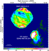 |
Fig. 1 Radio view of SNR G46.8–0.3 at 1.4 GHz from combined THOR and VGPS continuum data (Beuther et al. 2016). The colour scale varies linearly and is in units of mJy beam−1. The angular resolution is 25′′ and the sensitivity is 0.72 mJy beam−1. The bright source at the southwest corner is the H ii region named G046.495–00.241 in the WISE Catalog of Galactic H ii Regions (Anderson et al. 2014). |
3.1 Global Radio Continuum Spectrum
We updated the integrated radio continuum spectrum of G46.8–0.3. For this purpose, we measured flux densities over the whole extension of the source using publicly available images at low-radio frequencies from GLEAM, along with others at higher frequencies from THOR+VGPS, and GB6 (details of these observations are in Sect. 2.1), and the Radio Continuum Survey of the Galactic Plane at 10 GHz made with the Nobeyama Radio Observatory (NRO, HPBW ~2′.7, rms ~ 33 mJy beam−1, Handa et al. 1987). We also combined our new flux determinations with a carefully selected set of previously published estimates. While compiling these data, we rejected flux measurements previously reported with error estimates greater than 20%, as well as data points showing a large scatter beyond the range of 2σ best-fit values.
In our study, we also adopted the absolute flux density scale presented by Perley & Butler (2017) to tied fluxes for frequencies between 50 MHz and 50 GHz, the range where the scale is accurate to 3% and up to 5% for measurements at the extreme frequency values. Table 1 contains all the flux density values for G46.8–0.3 covering about 2.5 decades in frequency from 30.9 MHz to 11.2 GHz. Only three fluxes in our list were not adjusted to this common scale because of the lack of information about the calibrator sources in the original publications.
The integrated spectrum of G46.8–0.3 at radio frequencies that we created is plotted in Fig. 2. The weighted best fit to the data corresponds to a single power-law slope α = −0.535 ± 0.012 (Sv ∝ vα). This integrated spectral index is compatible with what is expected for a middle-aged shell-type SNR accelerating radio-emitting electrons via a first-order Fermi mechanism. Compared with previous determinations made for G46.8–0.3, our result is largely consistent with those by Kovalenko et al. (1994b; α = −0.53 ± 0.10), Dubner et al. (1996; α ~ −0.53), and Sun et al. (2011; α = −0.54 ± 0.02), but is flatter than the spectra measured by Kassim (1989a; α ~ −0.6) and Taylor et al. (1992; α = −0.72 ± 0.14, estimated using only flux density values at 327 MHz and 4.8 GHz). We consider that our spectrum notably improves on the previous ones published for G46.8–0.3, most of them with larger relative error in the spectral index determination. This is essentially a consequence of the fact that we have filled gaps along the radio frequency domain by compiling twice as many flux density values as Kovalenko et al. (1994b) and Sun et al. (2011), as well as setting the majority of the measurements to the most accurate absolute flux density scale presented to date.
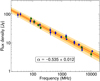 |
Fig. 2 Updated integrated radio continuum spectrum of SNR G46.8–0.3 constructed using fluxes listed in Table 1. Blue circles correspond to fluxes extracted from the literature, whereas the green squares are our new measurements obtained from radio surveys (see text for details). The solid line is the best-fitting curve to the weighted data and yields a spectral index α = −0.535 ± 0.012 (Sv ∝ vα). Shaded regions represent the variation of the best-fit values at 1- and 2-σ levels. |
3.2 Local Variations of the Spectral Index Across G46.8–0.3
We present the spectral index maps between 200 MHz and 1.4 GHz and between 1.4 GHz and 4.8 GHz in Figs. 3a and b, respectively. An explanation of how these maps were constructed is presented in Sect. 2.1. Uncertainties for the local spectral index measurements on both maps are not higher than 0.1. We do not attempt to quantify the remaining parameter errors because we have no access to the collection of calibrated radio visibilities to match the data at each frequency before constructing the spectral maps. Nevertheless, the spectral images we are presenting here are still useful for tracing local trends in the radio domain. Some contours of the 12CO (J = 1–0) line emission are over-plotted on the spectral maps for reference.
As revealed in Fig. 3a, the distribution of spectral index values in the 200 MHz−1.4 GHz map is essentially flat, with a mean value a 0.3 over a horseshoe-like shape (in yellow-greenish shaded) that seems to align with the molecular material into which the SNR shock front is running, which is an issue we revisit in Sect. 5. The spectrum becomes slightly steeper (α ~ −0.45) towards the north portion of the remnant. By comparison, the spectral indices between 1.4 and 4.8 GHz appear to be more uniformly distributed and steeper than at lower frequencies ranging from 200 MHz to 1.4 GHz. A moderately flatter spot (α ~ −0.5) is also noticeable in the 1.4/4.8 GHz map towards the eastern side of G46.8–0.3.
There seems to be a general trend in our spectral index maps of a slight concave-down behaviour (i.e. a steeper spectrum to higher radio frequencies). We recognise that the maps do not have sufficient sensitivity to be able to decipher whether or not this signature primarily occurs in the brightest portions of the remnant. If so, it might be a consequence of a higher effective shock compression undergone by low-frequency electrons in the interaction with adjacent clouds, which can cause local increases in the magnetic field strength and/or the particle density. Even if this scenario is true for the case of G46.8–0.3 it has no measurable effect on the integrated spectrum of the source, which as shown in Sect. 3.1 is well fitted by a single power law (see Fig. 2). There are a few cases of SNRs showing a steepening at high radio frequencies in their integrated spectra, with frequency cut values varying from at around a few MHz up to GHz (e.g. Galactic SNRs S147, Xiao et al. 2008 and HB 21, Pivato et al. 2013, and J0527–6549 in the Large Magellanic Cloud, Bozzetto et al. 2010). All of them are evolved SNRs for which the observed global spectral form was explained in the standard diffusive acceleration shock theory by the compression of the Galactic magnetic field in dense interstellar regions combined or not with a possible contribution of synchrotron losses of the high-energy electrons (see Urošević 2014 and Xiao et al. 2008 for a review of this subject). However, we consider the occurrence of synchrotron losses in G46.8–0.3 unlikely. Indeed, the radiative cooling time of GeV electrons producing radio synchrotron emission in a magnetic field B scales as tsyn ~ 1.3 × 10¹⁰ (B/µG)−2 (E/GeV)−1 yr (Gaisser et al. 1998) and in the case of G46.8–0.3 is found to be tsyn ~ 5 × 10⁶ yr. In this calculation, we assume E = 3 GeV for the energy of the electrons, along with an interstellar magnetic field strength in the clouds of BISM ≃ n1/2 µG (Hollenbach & McKee 1989) and B = 4BISM ~ 30 µG in the upstream region because of the shock compression in a gas with a mean molecular hydrogen density n ~ 50 cm−3 (obtained from Table 2 presented below). We notice that our tsyn estimate is absolutely comparable with typical values derived for SNRs evolving in relatively dense ambient medium (see e.g. Fig. 5.3 in Aharonian 2004). However, as we show in Sect. 4.2, it is much larger than the age of the SNR (tSNR ~ 1 × 10⁴ yr). More sensitive radio observations towards G46.8–0.3, particularly at the low-frequency band, are required to confirm the validity of our analysis of local variations in the spectral index before coming to any firm conclusions.
4 Results of the H i Data
Figure 4 displays the HI intensity in a velocity range from 10 to 66 km s−1 superposed on the 1.4 GHz radio continuum emission from G46.8–0.3 and the nearby HII region G046.495–00.241.
The interstellar hydrogen appears to be distributed all around the rim of G46.8–0.3 throughout the velocity interval presented in Fig. 4. Over the SNR shell, the brightness temperature of the HI decreases significantly as compared with values observed outside the G46.8–0.3 boundary. There are HI local depressions, which are especially noticeable towards the northern and southern parts of the SNR shell. We checked that the spectra extracted from these regions show clear signs of absorption. Due to their morphological correspondences with the brightness continuum emission from the remnant, we argue that these features correspond to absorbing atomic gas located in front of G46.8–0.3 relative to the line of sight. There is also a faint belt-like feature of H i, seen for velocities greater than ~30 km s−1 crossing the remnant from northeast to northwest. We find no signs of strong absorption (only a 3σ signal) in the H i profiles (not presented here) obtained in this region. Of course, the low surface brightness of the remnant could be limiting the absorption, but also means that most of the atomic gas forming the belt-like feature could be placed on the far side of the SNR. In the southwest of the remnant, the H i is seen in absorption against the continuum radiation from the nearby H ii region G046.495–00.241.
In summary, the distribution of the neutral gas towards G46.8–0.3 does not show evidence for neighbouring structures that may have been impacted by the SN shock. In addition, no signatures for material swept up due to the activity of the remnant or its progenitor are observed. If an expanding H i structure were present, it would be observed in a reduced velocity interval of the atomic distribution as a region of low emission surrounded by a shell completely or partially correlated with the outer boundary of the SNR. A structure of this kind is not observed in the case of G46.8–0.3. Our analysis based on VGPS data confirms the previous result obtained by Park et al. (2013) in the direction of G46.8–0.3 using lower spatial resolution (HPBW = 3′.35) 21 cm line data from the Inner-Galaxy Arecibo L-band Feed Array (I-GALFA) H i survey (Gibson et al. 2012).
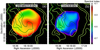 |
Fig. 3 Spectral index maps for SNR G46.8–0.3 constructed between (a) 200 MHz and 1.4 GHz and (b) 1.4 and 4.8 GHz. The images used are from GLEAM, THOR+VGPS, and GB6 surveys (see Sect. 2.1). Regions with flux densities lower than 4σ level of the respective rms noise in each image were clipped. The colour scale displayed to the right indicates the spectral index measured (with a 4′ resolution) over the SNR at both frequency bands. Dark and light green contours represent the intensity of the FUGIN 12CO (J = 1–0) molecular line emission (at a 2′ spatial resolution) integrated in the 30–50 km s−1 (levels: 500 and 800 K km s−1) and 50–66 km s−1 (levels: 1100 and 1400 K km s−1) ranges, respectively. A detailed treatment of the molecular features associated with G46.8–0.3 is presented in Sect. 5. |
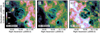 |
Fig. 4 Velocity channel maps of the H i emission in SNR G46.8–0.3 from VGPS spectral line data overplotted with the THOR+VGPS contours (levels: 70, 120, and 150 mJy beam−1) of the radio continuum radiation from the remnant and the H ii region G046.495–00.241. For comparison, the radio continuum image was smoothed to the 60′′ spatial resolution of the H i data. Before constructing the maps presented in the figure, an appropriate mean background level was subtracted from each H i velocity channel. The integration velocity range is indicated in the bottom left corner of each panel. All the velocity ranges are displayed with the linear colour scale in units of K km s−1 shown in panel a. |
4.1 Newly Derived Distance for SNR G46.8–0.3 and the Nearby H ii Region G046.495-00.241
There is no agreement on the estimates for the distance to G46.8–0.3 reported in the literature. Sato (1979) suggested a distance between 6.8 and 8.6 kpc from the analysis of H i absorption. Later, Ranasinghe & Leahy (2018) from the analysis of H i spectral features, proposed lower and upper limits of the distance of 5.7 and 11.4 kpc. More recently, Liu et al. (2019) listed a distance of 6.4 kpc through the detection of a hydrogen radio recombination line (RRL) using data from the Survey of Ionized Gas of the Galaxy carried out with the Arecibo telescope (SIGGMA, Liu et al. 2013).
In order to improve the distance estimate to our target and to obtain a more complete picture of the physical association with the rich ambient medium – which we discuss later in Sect. 5 –, we begin with a discussion of the properties of the H i spectrum seen against the remnant. To do so, we used the H i cube from the VGPS. Figure 5a shows H i emission and absorption profiles for G46.8–0.3. The emission spectrum was obtained in the line of sight directly towards the bright southern portion of the source, while the absorption spectrum was constructed by subtracting the emission profile from a spectrum averaged over a set of regions close to the remnant. Firstly, we mention that the absence of any absorption feature at negative velocities in the spectrum5 means that the SNR is inside the solar circle. Thus, according to the circular rotation curve model of the Galaxy by Reid et al. (2014), an upper limit on the distance of ~11.4 kpc (which approximately corresponds to a radial velocity of 0 km s−1) can be established. Secondly, we detect absorption up to the velocity of the tangent point, which at the longitude of the SNR is around 65 km s−1 (Reid et al. 2014). This represents a lower limit on the distance of ~5.7 kpc. The H i absorption beyond the tangent point velocity probably corresponds to velocity perturbations near the tangent point, caused for instance by expansion of the SNR. Additionally, we stress that significant and continuous absorption is observed from the velocity of ~ 40.4 km s−1 to that of the tangent point, which might even imply that a better estimate of the minimum distance is the far side distance for ~40.4 km s−1. Therefore, we assign a kinematic distance of 8.7 ± 1.0 kpc to the remnant. The error in our measurement is primarily caused by uncertainties in determining radial velocities along the line of sight, departures from circular motions of the Galaxy, as well as uncertainties associated with the selection of the rotation curve and solar motion. All of these contributions were added in quadrature in our calculations.
Now, we turn our attention to the H ii region G046.495–00.241 seen in the area mapped in Fig. 1 as a bright source with an angular diameter of ~7′. The centre of this source and that of the remnant are separated from each other by approximately ~16′.4. In order to revisit the kinematic distance to G046.495–00.241, in Fig. 5b we present absorption and emission profiles that we have constructed using spectral line VGPS observations directed to the central portion over the thermal source. The velocity for the H ii region deduced in Liu et al. (2019) from hydrogen RRL is 58.4 km s−1. The corresponding near and far distances inferred with the rotation curve of Reid et al. (2014) are 4.2 and 7.3 kpc, respectively. As revealed in Fig. 5b, the H i spectrum exhibits absorption at the ~4σ level beyond the RRL velocity up to the velocity of the tangent point, which at the Galactic longitude of the H ii region is ~65.6 km s−1. Therefore, we placed the thermal source at the far distance of 7.3 ± 1.2 kpc, in accordance with the distance that we established in Sect. 5 to the molecular emission spatially coincident with it. We find that our distance determination is markedly consistent with the 7.8 kpc value reported by Quireza et al. (2006) from measurements of intensity and width in helium RRL data, but incompatible with those provided by Kuchar & Bania (1990) (d = 3.9 kpc) obtained using H i absorption spectrum with data from the Boston University-Arecibo Galactic H i Survey, Anderson & Bania (2009; d = 3.8 ± 0.6 kpc) based on a combination of H i and CO sky surveys, and Anderson et al. (2014; d = 4.7 ± 0.1 kpc) in their WISE census of H ii.
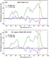 |
Fig. 5 H i line emission (green curve) and absorption (violet curve) spectra against (a) G46.8–0.3 SNR and (b) G046.495-00.241 H ii region. The solid vertical line in each panel marks the velocity of the tangent point at the longitude of the sources according to the Reid et al. (2014) Galactic rotation curve, whereas the dashed vertical line in panel b is for the hydrogen RRL at 58.4 km s−1 from G046.495–00.241 recorded in Liu et al. (2019). The horizontal shaded regions indicate the rms noise level of ~4 K in the H i absorption spectra. |
4.2 Age Estimate for G46.8–0.3
Taking into consideration the 8.7 ± 1.0 kpc distance to G46.8–0.3 that we determined in this work and its angular radius ≃8′.5 measured from the 1.4 GHz THOR+VGPS image, the physical radius of the SNR is approximately RSNR ≃ 21.5 pc. We used this result to estimate the dynamical age of the remnant by employing evolutionary models. To this end, we note that in surveys such as VTSS6 (Dennison et al. 1998), DSS7, APASS8, or IPHAS9 (Barentsen et al. 2014) there is no appreciable optical emission in apparent association with G46.8–0.3, indicative of radiative shocks. Also, no X-ray emission was detected associated with the SNR in the only observation (~9.9 ks) for this remnant available in the Chandra Data Archive10. Nevertheless, although it is not a strong constraint on age, the large size of G46.8–0.3 could suggest that it is an evolved object. Under this interpretation, we hypothesise that the remnant is in the later adiabatic expansion stage of its evolution. We caution that, although it can be reliable in terms of the order of magnitude, our modest estimation of the age of G46.8–0.3 suffers from large uncertainties derived from the assumed parameter values and the assumption of its current evolutionary stage. According to the numerical approach of Cox (1972), for a Sedov-Taylor (ST) blast wave shock with a specific heat ratio γ = 5/3, the age for G46.8–0.3 given by tsnr = 14.5(Rsnr)5/2(n0/E51)1/2 is about  yr. In the calculations above, E51 is the kinetic energy of the explosion normalised to the canonical value 1051 erg, assumed to be E51 = 1 in this work11, while n0 is the pre-shock number density for which we adopted n0 ~ 0.1 cm−3, a value of reference between a typical density inside a wind bubble excavated by the stellar progenitor (n0 ~ 0.01 cm−3) and that of the diffuse inter-cloud gas (n0 ~ 1 cm−3) (Inoue et al. 2012). In addition, the expansion velocity of the SN shock during the adiabatic phase is
  . Following the approach presented by Blondin et al. (1998), the transition time to the radiative phase will occur at
  , with a velocity of the shock wave
  .
.
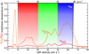 |
Fig. 6 Overall CO spectra covering the SNR G46.8–0.3 region. The three shaded areas correspond to LSR velocity ranges for which there is good spatial correspondence between the molecular matter and the remnant (see discussion in the text). The velocity of the tangent point (~65 km s−1, Reid et al. 2014) is marked with a black vertical line. |
5 Results of the CO Data
5.1 Morphology of the CO Molecular Gas Components
Figure 6 depicts the average spectrum of the 12CO and 13CO ( J = 1–0) molecular lines over a circular region of radius 14′ concentric with the remnant G46.8–0.3. Multiple velocity components are evident towards the SNR in the range of ~10–65 km s−1. In what follows, we investigate the spatial distribution of the molecular gas around G46.8–0.3 traced by CO isotopologues, leaving a discussion of the spectral characteristics of the molecular ambient matter to Sect. 5.2. We have omitted the analysis of the molecular gas responsible for the very narrow (FWHM ∆υ ≃ 2.5 km s−1) emission feature at ~7 km s−1 because we find no evidence of association with the SNR.
In Fig. 7, we present three-colour integrated intensity maps of the molecular environments in the direction of G46.8–0.3 (12CO J = 1–0 in red and13 CO J = 1–0 in green) obtained by FUGIN, together with the SNR radio synchrotron emission at 1.4 GHz (in blue) as traced by THOR+VGPS data. In such a representation, 12CO observations typically delineate emission mostly coming from low-density gas in the outer layers of the cloud, while the 13CO data generally trace optically thin emission from denser regions. The mapped CO emissions correspond to molecular structures for which we consider there is a convincing match with the remnant. They are in three velocity intervals: 10–30 km s−1, 30–50 km s−1, and 50–66 km s−1. The molecular matter in these velocity intervals is hereafter referred to as Regions A, B, and C, respectively. According to their kinematical properties, which are analysed in detail in Sect. 5.2, the regions are also separated into subareas or clouds. In the notation adopted throughout this work12, each cloud is labelled with a capital letter (A, B, or C), a number referencing the distance to the cloud, and the letters N, E, W, SW, or C depending on whether the cloud is located to the north, east, west, or southwest of the remnant or at its centre, while the H ii abbreviation is added for the gas immersed in the G046.495–00.241 region.
As shown in Fig. 7a, the gas in Region A at velocities in the 10–30 km s−1 range comprises two molecular components distributed around the SNR shell. These are: (i) the cloud named A-10N and (ii) the cloud A-10SW. The former closely follows the northern edge of the remnant. In addition, part of this gas appears to be projectionally embedded in the synchrotron emission fromthe remnant encompassing a distortion observed in the outer envelope of the SNR shell at the position RA ~ 19h17m45s, Dec ~ 12°15′40′′. This correspondence is compatible with a shock wave of the SNR interacting with the ambient matter. The molecular concentration also extends outside the northern limb of the remnant towards the southwest. The second molecular component, labelled A-10SW, consists of a set of clumps concentrated on the southwest edge of the SNR, exactly at the site where the shock front is flattened.
For intermediate velocities, 30–50 km s−1, the ambient medium in Region B can be divided into three main zones (Fig. 7b): (i) the molecular concentration towards the east, including the clouds B-3E and B-8E, which correlates with the limb of the remnant and extends out about 20′ in the northeast direction beyond the shock front; (ii) the molecular gas distributed in the interior of the SNR shell in a northeast-southwest orientation, labelled cloud B-9C, which appears to pass through bright patches of the radio continuum emission; and (iii) the western region comprising clouds B-3W and B-8W, which seems to be part of a molecular wall in the environment of our target source.
At the highest velocities, 50–66 km s−1, there is molecular gas seen in projection all around the remnant (Fig. 7c). The best match is observed towards the east where the CO in the C-6E region closely follows the edge of G46.8–0.3. The spatial correlation with the remnant decreases in the western half of the map, where the cloud C-4W is observed outside the SNR shock front, but still around it. Towards the southwest is the molecular gas concentration named C-7.5HII, probably the birthplace of the star-forming H ii region G046.495–00.241.
Figure 7 also reveals that all the identified molecular regions contain multiple enhancements where the 13CO J = 1–0 line emission is detected at levels higher than 5σ in coincidence with local maxima in the 12CO emission. The 13CO excess noticeable in the clouds A-10N, A-10SW, B-8E, and B-9C seen in projection onto the radio shell of G46.8–0.3 may indicate strong compression of the molecular gas due to interaction with the SNR shock front.
At first glance, G46.8–0.3 seems to be embedded within a dense molecular cavity. The existence of an almost complete COline cavity at 52 km s−1 associated with the remnant was already proposed by Sofue et al. (2021) based on the FUGIN survey of 12CO- and 13CO (J = 1–0)-line channel maps, the same data we used in the current work. These authors did not determine the kinematic distance to the structure but mentioned possible near and far values of 3.9 and 7.1 kpc, respectively. On the basis of an CO–H i combined spectral analysis, in the following section we determine the distance to each molecular structure unveiled in our work and hence we revisit the hypothesis of a cavity in the molecular medium around G46.8–0.3.
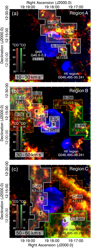 |
Fig. 7 Colour representation of the molecular ambient gas towards SNR G46.8–0.3 traced by the 12CO J = 1–0 (in red) and the 13CO J = 1–0 (in green) rotational line emissions. Yellow regions are areas where both CO isotope emissions overlap. The SNR radio continuum radiation at 1.4 GHz from THOR+VGPS surveys is represented in blue. The velocity range used to integrate the CO intensity is shown in the bottom left corner of each panel. The name of the discovered molecular features and their kinematic distances are also labelled. White continuous polygons enclose structures associated with G46.8–0.3. Non-associated clouds localised at the far distance of their central velocity are encircled by green continuous polygons, whereas foreground molecular gas along the line of sight is inside orange dashed polygons. Numbers from 1 to 9 spread out in panels a–c indicate the test regions used to construct the spectra presented in Fig. 8. |
5.2 Kinematics of the CO Molecular Gas Components
Here, we focus on determining the kinematic distances to the uncovered molecular structures comprising regions A-C shown in Fig. 7. To achieve this we extracted multiple H i and CO emission and absorption spectra covering the complete extension of each cloud, some of which are presented in Fig. 8. The test areas corresponding to our examples are marked with numbers from 1 to 9 in Fig. 7. In Table 2, we report average physical properties (peak intensity, velocity, line-width, angular size, column density, mass, and number density) computed over each CO structure unveiled in this work. Column densities and masses were calculated from the expressions presented in Sect. 2.2 and using the distance estimates provided here.
The sources of uncertainty in our distance results computed from CO–H i combined spectra are the same as those of our distance determination to the SNR and the H ii region derived in Sect. 4.1 from H i profiles only. As listed in Table 2, the final error in the measured distances to the molecular clouds is better than 10%, with the exception of those located at the near-side or close to the tangent point, for which the mean error is ~33%. On the other side, the final error in the measured distances to the molecular clouds combined with both the error of at least 30% in the CO-to-H2 conversion factor (Bolatto et al. 2013) and the uncertainties in isolating overlapping regions of sky translate into errors in the calculated properties (i.e. column densities of each velocity component and mass) of the interstellar gas. See further details in Table 2.
5.2.1 Region A: 10–30 km s−1
Now, we analyse the molecular gas inside Region A, spatially correlated with the northern and the southwestern edges of G46.8–0.3 (Fig. 7a). The spectra corresponding to the selected areas over this region appear in Figs. 8a, b. The excellent correspondence between the southern part of the molecular gas emission from the cloud named A-10N and the 1.4 GHz brightest emission from G46.8–0.3 is consistent with an interaction zone between the remnant and its immediate environment. If so, the distance to the molecular region should agree with that established for the SNR (8.7 ± 1.0 kpc, see Sect. 4.1). The 12CO spectrum over the A-10N cloud seen (in projection) immersed in the radio shell of the SNR exhibits a peak at ~15 km s−1 with a 13CO counterpart. Using the flat rotation curve model of Reid et al. (2014), the kinematic distances associated with this velocity are 1.0 and 10.2 kpc. In addition, the H i 21 cm profile in the molecular component exhibits dips corresponding to CO emission lines at velocities up to the velocity of the tangent point, the maximum velocity that the foreground clouds can have. The observed CO-H i anti-correlation can be explained in terms of foreground molecular clouds along the line of sight absorbing the continuum radiation from the SNR (Roman-Duval et al. 2009). Therefore, we assigned a far side distance of 10.2 ± 0.7 kpc to the investigated cloud. If the cloud were located at the near position of its velocity, absorbed features would be observed in the H i profile correlated with CO emission lines up to the velocity of the clump only. We also notice the 12CO line profiles in Region A deviate to higher velocities relative to the 13CO line maximum intensity. This is not surprising, as the latter is a more faithful tracer of the denser regions in the molecular gas. At this stage, we note that the spectra (not presented here) constructed over the molecular gas extending beyond the SNR boundary confirm that the A-10N cloud is a single structure placed at ~10 kpc. Therefore, taking into consideration that we have established the location of the SNR at 8.7 ± 1.0 kpc, we interpret the asymmetry in the 12CO line emission (line FWHM Δυ ≃ 6.5 km s−1) as a sign of perturbation caused by the SNR shock wave penetrating into the most massive (~214 × 103 M⊙) cloud interacting with G46.8–0.3, which is physically located at the backside of the remnant. The striking morphological correspondence between the molecular gas and the radio boundary also further supports the shock-cloud interaction idea.
Upon inspection of the molecular gas in Region A, we noticed that the spectra constructed over the western extreme of the northern cloud, that is, where it curves to the south (at RA ~ 19h17m15s, Dec ~ 12°15′20′′, see Fig. 7a), display a CO emission peak at ~16 km s−1 correlated with H i self-absorption against warm 21 cm backgrounds (emitting at the same velocity as the cloud). This behaviour implies that this part of the surveyed Region A, referred to as A-1N, is at the near distance of 1.1 ± 0.6 kpc. We estimated that the mass of this gas only represents a small fraction (<1%) of the molecular material in the north brightening in the velocity range 10–30 km s−1.
As shown in Fig. 7a, the molecular gas in Region A also comprises bright clumps in the southwest (cloud A-10SW), where the rim of G46.8–0.3 clearly deviates from a circular geometry. The CO profile presented in Fig. 8b was obtained in a test area just outside the SNR over the clump with a central velocity of ~19 km s−1. The correlation of the CO peak with a maximum in the H i emission indicates that this part of the molecular region resides at the far position of 10.1 ± 0.6 kpc.
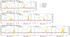 |
Fig. 8 Collection of composite spectra of the CO (j = 1–0) and H i 21 cm line emissions towards test areas over the molecular structures discovered in the direction of SNR G46.8–0.3, as shown in Fig. 7. The correspondences between the molecular and atomic emissions were used to determine the kinematic distance to individual clouds (see analysis in Sect. 5.2). The shaded zones in yellow highlight the CO peak and the LSR velocity in the region we are interested in. The blue vertical line in each spectrum indicates the velocity of the tangent point according to the rotation curve model of Reid et al. (2014). For the remaining spectra (not shown here) used in our analysis, we found approximately the same behaviour in each region as that exhibited by the spectra presented here. |
5.2.2 Region B: 30–50 km s−1
Over the CO material brightening between 30 and 50 km s−1 in the eastern area outside the remnant we find spectra showing H i self-absorption features at ~41 km s−1 (Fig. 8c) and others revealing CO peak intensities at ~48 km s−1 coincident with H i maxima (Fig. 8d). This means that the ambient matter eastwards of G46.8–0.3 results from a chance coincidence of near-side (cloud B-3E at 2.8 ± 0.8 kpc) and far-side (cloud B-8E at 8.2 ± 0.7 kpc) components superposed along the line of sight. At RA ~ 19h18m30s, Dec ~ 12°13′00′′, the molecular emission bends to the west and overlaps the eastern portion of G46.8–0.3. The spectral properties over this zone (spectra not included in Fig. 8) indicate that it is an extension of the molecular material outside G46.8–0.3. Indeed, for the near-side gas, the cold H i embedded in the foreground molecular clouds absorbs the continuum radiation from the SNR and produces spectral H i 21 cm absorption lines up to a velocity of around 41 km s−1 of the material we are interested in, while over the far-side, component H i 21 cm valleys corresponding to CO emission line features are observed up to the velocity of the tangent point. We also estimated that the amount of gas in the near-side component constitutes -10% of the total material in the eastern region shown in Fig. 7b. As opposed to the incidental near- and far-side overlap of the CO structures in the east of the SNR, the spectral properties of the central B-9C cloud, which appears embedded in the SNR shell (RA ~ 19h18m00s, Dec ~ 12°06′10′′) at a velocity of about 40 km s−1, allow us to conclude that it corresponds to a single cloud at the far kinematic distance of 8.7 ± 0.6 kpc. As an example, Fig. 8e presents a spectrum extracted over this central area. The obtained distance to the cloud is fully compatible with the distance we measured for G46.8–0.3 and therefore we interpret the enhanced filaments of radio continuum emission as a trace of the SNR shock impacting on the relatively dense (~40 cm−3) B-9C cloud. It is worth mentioning that we find little evidence of disturbance in the profiles of the CO extracted over the molecular gas superimposed on the remnant. However, this result does not rule out an association with G46.8–0.3.
Finally, we mention that near and far molecular components with line-of-sight coincidence were detected westwards of G46.8–0.3 at a velocity of ~48 km s−1 (spectra not shown here). These cloud components are inside the regions we denote B-3W and B-8W, respectively. As shown in Fig. 7b, this ambient medium was not overtaken by the SNR shock. We determined that approximately only 3% of the surveyed gas in the west is at the near position of 3.3 ± 0.9 kpc forming the cloud B-3W, while the remaining material is at 8.2 ± 0.7 kpc inside the cloud B-8W (see Table 2).
Measured and derived properties for the molecular structures identified in the direction of SNR G46.8–0.3.
5.2.3 Region C: 50–66 km s−1
To analyse the molecular material in Region C we divided it into three areas of differing spectral properties. The first zone comprises the gas forming the large eastwards structure (cloud C-6E). Towards the western half of the field is the second molecular component (namely C-4W zone). In this region, at a distance of up to ~18′ from G46.8–0.3, the CO (J = 1–0) line emission is significantly detected from RA ~ 19h17m45s, Dec ~ 12°27′00′′ to RA ~ 19h17m00s, Dec ~ 12°00′00′′ (see Fig. 7c). Lastly, the third important area corresponds to the gas seen projected onto the G046.495–00.241 H ii region (the C-7.5HII cloud). Before describing the spectra, we point out that because of the small velocity difference measured in the profiles of the C-6E and C-4W areas between their CO peaks and the tangent point (υTP ~65 km s−1, derived from the Reid et al. 2014 model) it is not simple to conclusively determine whether the clouds are at the near or the far position. Even though arguments based on morphological correlations and spectral correspondences between the CO and H i gases indeed may help to estimate their locations along the line of sight, the uncertainties are significantly larger than those associated with the A and B clouds. Therefore, our interpretation of the spectral features obtained over the east and west areas in Region C should be regarded with care. As we discuss below, the situation is different for the C-7.5HII zone because the HII region – whose distance was determined in Sect. 4.1 – sits inside the molecular gas.
The CO profiles over the portion of the cloud C-6E superposed on the SNR shell show maxima at around 64 km s−1 correlated with H i absorption dips. This spectral condition (observed at almost the same velocity as that of the tangent point) could indicate that the molecular emission occurs at a kinematic distance of 6.3 ± 2.0 kpc associated with the mean central velocity measured in the region. This estimate is, within uncertainties, in reasonable agreement with the distance to G46.8–0.3. A key point to note is that many of the spectra we constructed over the narrow portion of the C-6E cloud superposed on G46.8–0.3 were found to be broadened (FWHM line Δυ ~ 9 km s−1; see example in Fig. 8f). Analogous spectral features have been found in other known SNR-molecular cloud interactions and were interpreted as the result of turbulent motions in the shocked gas (e.g. W44, Seta et al. 2004; G347.3–0.5, Moriguchi et al. 2005; Kes 69, Zhou et al. 2009; G357.7+0.3, Rho et al. 2017; HB 3, Rho et al. 2021). We also found a similar line broadening in the CO spectra constructed over the portion of the C-6E cloud immediately outside the SNR forward shock. In this case, the spectra exhibit strong CO emission lines with peak intensities at around ~63 km s−1 without associated H i self-absorption features (see the representative profiles in Fig. 8g). Therefore, from our spectral analysis on the C-6E region we conclude that it is a single cloud located at 6.3 ± 2.0 kpc. Taking into account the distance we measure to G46.8–0.3 and the large uncertainties in our distance determination to the molecular gas in the C-6E zone, we cannot completely discard the possibility that the cloud is located in the immediate foreground relative to the SNR. The good spatial agreement of C-6E with the outer part of the remnant may be considered additional evidence for a possible physical relationship between them.
Interestingly, we find that the spectral properties over the western part of Region C change from those observed in the east. Indeed, the profiles extracted over the gas forming the C-4W cloud display CO peaks at a mean central velocity of ~58 km s−1, and all of them are correlated with H i absorption dips (Fig. 8h). We interpret this result as indicative of cold H i gas within a molecular structure placed at the near distance of 4.2 ± 1.8 kpc, which is absorbing the warmer H i emission from the ISM at the same velocity as the CO cloud. Regarding the C-7.5HII zone, where the CO emission is brightest, the spectra present a peak at ~56 km s−1 with broad emission lines of ~ 9 km s−1 (see e.g. Fig. 8i). The position of the maximum CO intensity in accordance with both the radio recombination line velocity of the H ii region (58 km s−1, Liu et al. 2019) and the atomic neutral gas seen in absorption against the background provided by the H ii region led us to conclude that the molecular gas in this region forms the natal cloud of the star formation activity in G046.495–00.241.
Finally, we point out that our detailed analysis of the spatial distribution of the molecular structures forming Region C (including clouds located over a large distance interval ~4–8 kpc) is not in agreement with the existence of a partial CO-line shell formed around G46.8–0.3 at the radial velocity of 52 km s−1, as proposed by Sofue et al. (2021). In their study, our target source is part of an extensive list made on the basis of morphological inspection, including the identification of approximately 60 candidates to molecular cavities and shells towards Galactic SNRs.
6 GeV γ-rays in the Field of G46.8–0.3
The latest version (Data Release 2) of the Fermi Large Area Telescope Fourth Source Catalogue (4FGL)13 records an 8.1σ detection of a γ-ray excess in the 100 MeV–1 TeV band, labelled 4FGL J1918.1+1215c, towards the eastern half of G46.8–0.3 (first report in Abdollahi et al. 2020). The spectrum of this source is well fit by a power law dN/dE = ϕ0E−Γ, with a differential flux ϕ0 = (1.59 ± 0.25) × 10−12 cm−2 s−1 MeV−1 at E0 = 1099 MeV and a photon index Γ = 2.65 ± 0.08, comparable to values measured in other SNRs with molecular cloud interactions (e.g. Kes 79, Auchettl et al. 2014; G290.1–0.8, Auchettl et al. 2015; W51C, Jogler & Funk 2016; W28, Cui et al. 2018).
Neither pulsars nor their associated wind nebulae are detected towards the γ-ray region in G46.8–0.3, which could explain the GeV emission. Motivated by the spatial correlation projected in the sky between the molecular cloud-SNR interaction zone and the Fermi source, we tested the possibility that the observed γ-ray flux results from neutral pion decay emission produced by collisions of hadronic cosmic rays with dense targets in the surrounding medium. To investigate this matter, given the limited spatial resolution of the γ-ray observations, we consider the large region ~30′ × 19′ in size corresponding to the 95% confidence level (CL) of the GeV source location (for comparison, the diameter of the SNR is ~17′). As illustrated in Fig. 9 the area of interest comprises portions of the molecular material embedded in the A-10N, B-8E, and B-9C ambient clouds unveiled in this work. To estimate the proton column density Np we computed the integrated column density of H2 from the 12CO line emission within the velocity ranges corresponding to these interacting clouds (see discussion in Sect. 5). Because of the uncertainty surrounding the association of G46.8–0.3 with the molecular material forming the C-6E region, we decided not to include any contribution from this matter in the following estimation. Using the relations presented in Sect. 2.2 we obtained  . We then estimated the proton density np = Np/L by adopting a path length L ~ 24′.5 ≃ 64 pc through the γ-ray emission, equivalent to the mean of the major and minor axes of the 95% CL ellipse that we assumed to be located at 9 kpc (i.e. the average distance for the interacting A-10N, B-8E, and B-9C molecular clouds; see Table 2). The resulting total proton content is therefore np ~100 cm−3. Regarding a possible contribution from the atomic gas phase, as the analysis of the H i distribution around the location of G46.8–0.3 did not reveal convincing structures associated with the source (see Sect. 4), it was not incorporated into the calculation above. For this reason, we are aware that the derived proton density for the GeV region represents a lower limit. When taking into account the contribution (integrated in the region of the molecular clouds) of the H i gas to the proton density, we find an increase of 30%. Nevertheless, the exclusion of the atomic component does not significantly change our conclusion presented below on the energetics of cosmic rays in the region of G46.8–0.3. We also mention that our analysis does not incorporate the contribution of the ionised hydrogen to the column density because we do not find significant IR counterparts in the region of interest.
The amount of energy injected into accelerated hadrons  can be estimated from the relation between the luminosity of the GeV source Lγ and the characteristic cooling time of protons through the neutral meson-production channel
  , which in turn depends on the proton density (Aharonian et al. 2006). At the adopted distance d = 9 kpc, we obtain Lγ(E > 1 GeV) = 4 π d2 wγ ≃ 5 × 1034 erg s−1, where wγ ≃ 5 × 10⁻¹² erg cm−2 s−1 is the γ-ray energy flux for E > 1 GeV. On the other hand, for the total proton density we measure in the 95% CL region of the Fermi detection, the cooling time of protons is found to be
  . Therefore, the total energy of cosmic rays required to produce the observed γ-ray flux in the region of SNR G46.8–0.3 is
  . This value for
  corresponds to ~ 0.2% of the canonical E ≃ 1051 erg SN energy and provides support to the interpretation that G46.8–0.3 could be the radio counterpart of the Fermi source produced via a hadronic process. We notice that a similar condition remains valid for a less conservative case of analysis in a smaller region corresponding to the 68% CL of the γ-ray detection.
Taking into account our estimation of the age of G46.8–0.3 and the properties of its environment revealed in this work, our value for  agrees well with those obtained for other interacting SNRs spatially correlated with γ-ray emission at GeV and/or TeV energies. We encourage the reader to consult the detailed information about this topic presented by Sano et al. (2021). It is important to note that though relatively simplistic, our analysis suggests that G46.8–0.3 is outside of the linear correlation proposed by these latter authors between the energy of cosmic-ray protons and the age of the accelerator. Certainly, the existence of any evolutionary tendency is an important issue that should be investigated on the basis of a larger sample of SNRs. Additionally, a more comprehensive study involving effects due to particle diffusion away from the SNR shell and/or re-acceleration of pre-existing cosmic rays inside the shock-compressed clouds is required in order to obtain a clearer picture of the γ-ray emission from G46.8–0.3.
Finally, with the abundant interstellar matter in the vicinity of G46.8–0.3 still in mind, we cautiously note that on the basis of the current information we have for the GeV γ-ray flux in the direction to the remnant, a contribution to the high-energy emission from bremsstrahlung γ-rays of relativistic electrons could also be likely. The critical aspect in modelling the occurrence of this physical process is the requirement of high electron-to-proton ratios of about 0.2, larger than the 0.01 value estimated from cosmic-ray abundances (Gaisser et al. 1998). Even with this caveat, there remain some examples in the literature where electron–electron or electron–ion interactions partially explain the γ-rays in the Fermi-LAT energy band via bremsstrahlung radiation (see e.g. Kes 41, Supan et al. 2018; HB21, Ambrogi et al. 2019). For the environment of the SNR G46.8–0.3, the cooling timescale due to bremsstrahlung losses is found to be tbr ≈ 4 × 10⁷ (np/cm3)−1 yr ≈ 4 × 10⁵ yr (Aharonian 2004). This is greater than the estimated age of the SNR (see Sect. 4.2) and leads to a realistic total relativistic particle energy of W ~ 6.3 × 1047 erg.
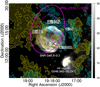 |
Fig. 9 Grey-scale image (in mJy beam−1) corresponding to the radio continuum emission from the shell of G46.8–0.3 overlaid with the 12CO (J = 1–0) line emission from Regions A (in cyan, Δυ = 10–30 km s−1, levels: 40, 70, 100 K km s−1) and B (in yellow, Δυ = 30–50 km s−1, levels: 55, 80, 105 K km s−1) around the SNR. The velocity range of the plotted clouds is the same as in Fig. 7. The plus symbol and ellipses illustrate the best localisation and the 95%/68% confidence contours of the γ-ray emission detected by Fermi-LAT. The enclosed molecular areas corresponding to the A-10N, B-8E, and B-9C clouds were used in Sect. 6 to calculate the total proton content. |
7 Summary and Conclusions
This work focuses on determining the properties of the radio continuum emission from the SNR G46.8–0.3, along with those of the atomic and molecular constituents in the surrounding medium. By assimilating new integrated flux densities that we measure from recently published 88–200 MHz GLEAM maps and others from surveys at 1.4, 4.8, and 10 GHz into a collection of data carefully selected from the literature, we have constructed the most complete version of the radio spectra for G46.8–0.3 available to date covering a broad range in frequency (30.9 MHz−11.2 GHz). A simple power law with an α = −0.535 ± 0.012 slope provides the best fit to the set of fluxes measured over the remnant in the radio domain. The straightness of the spectrum implies there is no ionised gas localised either inside the remnant, in its proximity, or in more distant ISM along the line of sight able to absorb the radio emission from G46.8–0.3, which would cause a deviation from a power law at the lowest frequencies. Although the integrated spectrum is well fit by a simple power law, our analysis of the local variations in the radio spectral index with position and frequency over G46.8–0.3 suggests a possible steepening at approximately 1 GHz. To determine the reality of any potential spectral curvature within small regions over G46.8–0.3, it is necessary to analyse high-quality radio data over a large frequency range correctly matched in the uv-domain.
No H i structures are found to be physically linked to G46.8–0.3. On the basis of neutral hydrogen absorption and emission spectra, we determine that the remnant is located at a distance of 8.7 ± 1.0 kpc, and from evolutionary models we also argue that G46.8–0.3 was created in a stellar explosion, likely occurring ~1 × 10⁴ yr ago.
Additionally, we provide for the first time a robust estimation of the distance to the molecular clouds lying in the direction of the SNR and present compelling signatures in the 12CO and 13CO (J = 1–0) line emissions of interaction between the forward shock of G46.8–0.3 and dense (with ~100 × 103 M⊙ and ~50 cm−3 average mass and density, respectively) molecular clouds distributed over the centre of the remnant, as well as along its northern, eastern, and southeastern edges. According to our findings, G46.8–0.3 can be added to the list of evolved remnants in our Galaxy with signs of interaction with molecular structures. Line emission observations of higher CO transitions with respect to the J = 1–0 rotational line are of interest to quantitatively analyse variations in CO line ratios resulting from both environmental and local shock conditions in the clouds. Unfortunately, at the time we made the analysis there were no images available from The CO High-Resolution Survey (COHRS) 12CO (J = 3–2) maps covering the complete extension of the remnant.
In line with the evidence we present in this work on the physical relationship between G46.8–0.3 and its surroundings, we also discuss an explanation of the γ-ray flux at GeV energies via neutral pion decay after hadronic collisions, which we find to be plausible as this process requires only a few percent of the total energy released in the stellar explosion creating G46.8–0.3. Furthermore, although very simplistic, our analysis also indicates that electron-dense medium interactions resulting in high-energy bremsstrahlung radiation cannot be conclusively ruled out at this stage. Compilation of the radio fluxes that we present here is necessary as an anchor at the lowest energies for the broadband spectral energy distribution of G46.8–0.3. Its inclusion is crucial to characterising the physical process responsible for the high-energy particle production in this remnant, which we demonstrate belongs to the reduced group of evolved interacting SNRs. Future γ-ray observations providing complementary data with increased sensitivity and spatial resolution in the multi-GeV Fermi energy range and at higher energies are also of interest in properly determining the spectral behaviour for G46.8–0.3.
Acknowledgements
The authors acknowledge the anonymous referee for his/her helpful comments. G. Castelletti and L. Supan are members of the Carrera del Investigador Científico of CONICET, Argentina. This work was supported by the ANPCyT (Argentina) research project with number BID PICT 2017-3320. Nobeyama Radio Observatory is a branch of the National Astronomical Observatory of Japan, National Institutes of Natural Sciences. Part of the data were retrieved from the JVO portal (http://jvo.nao.ac.jp/portal/) operated by ADC/NAOJ. The National Radio Astronomy Observatory is a facility of the National Science Foundation operated under cooperative agreement by Associated Universities, Inc.
References
- Abdollahi, S., Acero, F., Ackermann, M., et al. 2020, ApJS, 247, 33 [Google Scholar]
- Aharonian, F.A. 2004, Very high energy cosmic gamma radiation : a crucial window on the extreme Universe (World scientific Publishing Co. Pte Ltd) [CrossRef] [Google Scholar]
- Aharonian, F., Akhperjanian, A.G., Bazer-Bachi, A.R., et al. 2006, A&A, 449, 223 [NASA ADS] [CrossRef] [EDP Sciences] [Google Scholar]
- Altenhoff, W.J., Downes, D., Goad, L., Maxwell, A., & Rinehart, R. 1970, A&As, 1, 319 [NASA ADS] [Google Scholar]
- Ambrogi, L., Zanin, R., Casanova, S., et al. 2019, A&A, 623, A86 [NASA ADS] [CrossRef] [EDP Sciences] [Google Scholar]
- Anderson, L.D., & Bania, T.M. 2009, ApJ, 690, 706 [NASA ADS] [CrossRef] [Google Scholar]
- Anderson, L.D., Bania, T.M., Balser, D.S., et al. 2014, ApJS, 212, 1 [NASA ADS] [CrossRef] [Google Scholar]
- Angerhofer, P.E., Becker, R.H., & Kundu, M.R. 1977, A&A, 55, 11 [NASA ADS] [Google Scholar]
- Auchettl, K., Slane, P., & Castro, D. 2014, ApJ, 783, 32 [NASA ADS] [CrossRef] [Google Scholar]
- Auchettl, K., Slane, P., Castro, D., Foster, A.R., & Smith, R.K. 2015, ApJ, 810, 43 [NASA ADS] [CrossRef] [Google Scholar]
- Barentsen, G., Farnhill, H.J., Drew, J.E., et al. 2014, MNRAS, 444, 3230 [NASA ADS] [CrossRef] [Google Scholar]
- Beuther, H., Bihr, S., Rugel, M., et al. 2016, A&A, 595, A32 [NASA ADS] [CrossRef] [EDP Sciences] [Google Scholar]
- Blondin, J.M., Wright, E.B., Borkowski, K.J., & Reynolds, S.P. 1998, ApJ, 500, 342 [NASA ADS] [CrossRef] [Google Scholar]
- Bolatto, A.D., Wolfire, M., & Leroy, A.K. 2013, ARA&A, 51, 207 [CrossRef] [Google Scholar]
- Bozzetto, L.M., Filipovic, M.D., Crawford, E.J., et al. 2010, Serb. Astron. J., 181, 43 [NASA ADS] [CrossRef] [Google Scholar]
- Caswell, J.L., & Clark, D.H. 1975, Aust. J. Phys. Astrophys. Suppl., 37, 57 [NASA ADS] [Google Scholar]
- Chen, X., Xiong, F., & Yang, J. 2017, A&A, 604, A13 [NASA ADS] [CrossRef] [EDP Sciences] [Google Scholar]
- Chiotellis, A., Schure, K.M., & Vink, J. 2012, A&A, 537, A139 [NASA ADS] [CrossRef] [EDP Sciences] [Google Scholar]
- Condon, J.J., Broderick, J.J., & Seielstad, G.A. 1989, AJ, 97, 1064 [NASA ADS] [CrossRef] [Google Scholar]
- Cox, D.P. 1972, ApJ, 178, 159 [NASA ADS] [CrossRef] [Google Scholar]
- Cui, Y., Yeung, P.K.H., Tam, P.H.T., & Pühlhofer, G. 2018, ApJ, 860, 69 [NASA ADS] [CrossRef] [Google Scholar]
- Day, G.A., Warne, W.G., & Cooke, D.J. 1970, Aust. J. Phys. Astrophys. Suppl., 13, 11 [NASA ADS] [Google Scholar]
- Dennison, B., Simonetti, J.H., & Topasna, G.A. 1998, PASA, 15, 147 [NASA ADS] [CrossRef] [Google Scholar]
- Downes, D. 1971, AJ, 76, 305 [NASA ADS] [CrossRef] [Google Scholar]
- Dubner, G.M., Giacani, E.B., Goss, W.M., Moffett, D.A., & Holdaway, M. 1996, AJ, 111, 1304 [NASA ADS] [CrossRef] [Google Scholar]
- Gaisser, T.K., Protheroe, R.J., & Stanev, T. 1998, ApJ, 492, 219 [NASA ADS] [CrossRef] [Google Scholar]
- Gibson, S.J., Koo, B., Douglas, K.A., et al. 2012, in American Astronomical Society Meeting Abstracts, #219, 349.29 [NASA ADS] [Google Scholar]
- Green, D.A. 2019, J. Astrophys. Astron., 40, 36 [NASA ADS] [CrossRef] [Google Scholar]
- Gregory, P.C., Scott, W.K., Douglas, K., & Condon, J.J. 1996, ApJS, 103, 427 [NASA ADS] [CrossRef] [Google Scholar]
- Handa, T., Sofue, Y., Nakai, N., Hirabayashi, H., & Inoue, M. 1987, PASJ, 39, 709 [NASA ADS] [Google Scholar]
- Holden, D.J., & Caswell, J.L. 1969, MNRAS, 143, 407 [NASA ADS] [CrossRef] [Google Scholar]
- Hollenbach, D., & McKee, C.F. 1989, ApJ, 342, 306 [NASA ADS] [CrossRef] [Google Scholar]
- Hurley-Walker, N., Hancock, P.J., Franzen, T.M.O., et al. 2019, PASA, 36, e047 [NASA ADS] [CrossRef] [Google Scholar]
- Inoue, T., Yamazaki, R., Inutsuka, S.-I., & Fukui, Y. 2012, ApJ, 744, 71 [NASA ADS] [CrossRef] [Google Scholar]
- Jogler, T., & Funk, S. 2016, ApJ, 816, 100 [Google Scholar]
- Kassim, N.E. 1988, ApJS, 68, 715 [NASA ADS] [CrossRef] [Google Scholar]
- Kassim, N.E. 1989a, ApJ, 347, 915 [NASA ADS] [CrossRef] [Google Scholar]
- Kassim, N.E. 1989b, ApJS, 71, 799 [NASA ADS] [CrossRef] [Google Scholar]
- Kovalenko, A.V., Pynzar, A.V., & Udal'Tsov, V.A. 1994a, Astron. Rep., 38, 95 [NASA ADS] [Google Scholar]
- Kovalenko, A.V., Pynzar, A.V., & Udal'Tsov, V.A. 1994b, Astron. Rep., 38, 78 [NASA ADS] [Google Scholar]
- Kuchar, T.A., & Bania, T.M. 1990, ApJ, 352, 192 [NASA ADS] [CrossRef] [Google Scholar]
- Kuriki, M., Sano, H., Kuno, N., et al. 2018, ApJ, 864, 161 [Google Scholar]
- Leahy, D.A., Ranasinghe, S., & Gelowitz, M. 2020, ApJS, 248, 16 [NASA ADS] [CrossRef] [Google Scholar]
- Liu, B., McIntyre, T., Terzian, Y., et al. 2013, AJ, 146, 80 [NASA ADS] [CrossRef] [Google Scholar]
- Liu, Q.-C., Chen, Y., Chen, B.-Q., et al. 2018, ApJ, 859, 173 [NASA ADS] [CrossRef] [Google Scholar]
- Liu, B., Anderson, L.D., McIntyre, T., et al. 2019, ApJS, 240, 14 [NASA ADS] [CrossRef] [Google Scholar]
- Moran, M. 1965, MNRAS, 129, 447 [NASA ADS] [Google Scholar]
- Moriguchi, Y., Tamura, K., Tawara, Y., et al. 2005, ApJ, 631, 947 [NASA ADS] [CrossRef] [Google Scholar]
- Park, G., Koo, B.C., Gibson, S.J., et al. 2013, ApJ, 777, 14 [NASA ADS] [CrossRef] [Google Scholar]
- Perley, R.A., & Butler, B.J. 2017, ApJS, 230, 7 [NASA ADS] [CrossRef] [Google Scholar]
- Pivato, G., Hewitt, J.W., Tibaldo, L., et al. 2013, ApJ, 779, 179 [NASA ADS] [CrossRef] [Google Scholar]
- Quireza, C., Rood, R.T., Bania, T.M., Balser, D.S., & Maciel, W.J. 2006, ApJ, 653, 1226 [NASA ADS] [CrossRef] [Google Scholar]
- Ranasinghe, S., & Leahy, D.A. 2018, AJ, 155, 204 [NASA ADS] [CrossRef] [Google Scholar]
- Reid, M.J., Menten, K.M., Brunthaler, A., et al. 2014, ApJ, 783, 130 [NASA ADS] [CrossRef] [Google Scholar]
- Rho, J., Hewitt, J.W., Bieging, J., et al. 2017, ApJ, 834, 12 [Google Scholar]
- Rho, J., Jarrett, T.H., Tram, L.N., et al. 2021, ApJ, 917, 47 [NASA ADS] [CrossRef] [Google Scholar]
- Roman-Duval, J., Jackson, J.M., Heyer, M., et al. 2009, ApJ, 699, 1153 [CrossRef] [Google Scholar]
- Sano, H., Reynoso, E.M., Mitsuishi, I., et al. 2017, J. High Energy Astrophys., 15, 1 [NASA ADS] [CrossRef] [Google Scholar]
- Sano, H., Yamane, Y., Tokuda, K., et al. 2018, ApJ, 867, 7 [NASA ADS] [CrossRef] [Google Scholar]
- Sano, H., Rowell, G., Reynoso, E.M., et al. 2019, ApJ, 876, 37 [NASA ADS] [CrossRef] [Google Scholar]
- Sano, H., Inoue, T., Tokuda, K., et al. 2020a, ApJ, 904, L24 [NASA ADS] [CrossRef] [Google Scholar]
- Sano, H., Plucinsky, P.P., Bamba, A., et al. 2020b, ApJ, 902, 53 [CrossRef] [Google Scholar]
- Sano, H., Yoshiike, S., Yamane, Y., et al. 2021, ApJ, 919, 123 [NASA ADS] [CrossRef] [Google Scholar]
- Sato, F. 1979, Astrophys. Lett., 20, 43 [NASA ADS] [Google Scholar]
- Seta, M., Hasegawa, T., Sakamoto, S., et al. 2004, AJ, 127, 1098 [NASA ADS] [CrossRef] [Google Scholar]
- Sofue, Y., Kohno, M., & Umemoto, T. 2021, ApJS, 253, 17 [NASA ADS] [CrossRef] [Google Scholar]
- Stil, J.M., Taylor, A.R., Dickey, J.M., et al. 2006, AJ, 132, 1158 [NASA ADS] [CrossRef] [Google Scholar]
- Su, Y., Chen, Y., Yang, J., et al. 2009, ApJ, 694, 376 [NASA ADS] [CrossRef] [Google Scholar]
- Sun, X.H., Reich, P., Reich, W., et al. 2011, A&A, 536, A83 [NASA ADS] [CrossRef] [EDP Sciences] [Google Scholar]
- Supan, L., Castelletti, G., Supanitsky, A.D., & Burton, M.G. 2018, A&A, 619, A109 [NASA ADS] [CrossRef] [EDP Sciences] [Google Scholar]
- Tang, X. 2019, MNRAS, 482, 3843 [NASA ADS] [CrossRef] [Google Scholar]
- Taylor, A.R., Wallace, B.J., & Goss, W.M. 1992, AJ, 103, 931 [NASA ADS] [CrossRef] [Google Scholar]
- Trushkin, S.A. 1996, Bull. Spec. Astrophys. Observ., 41, 64 [Google Scholar]
- Umemoto, T., Minamidani, T., Kuno, N., et al. 2017, PASJ, 69, 78 [Google Scholar]
- Urosevi, C.D. 2014, Ap&SS, 354, 541 [NASA ADS] [CrossRef] [Google Scholar]
- Wayth, R.B., Lenc, E., Bell, M.E., et al. 2015, PASA, 32, e025 [NASA ADS] [CrossRef] [Google Scholar]
- Willis, A.G. 1973, A&A, 26, 237 [NASA ADS] [Google Scholar]
- Xiao, L., Fürst, E., Reich, W., & Han, J.L. 2008, A&A, 482, 783 [NASA ADS] [CrossRef] [EDP Sciences] [Google Scholar]
- Zhou, X., Chen, Y., Su, Y., & Yang, J. 2009, ApJ, 691, 516 [NASA ADS] [CrossRef] [Google Scholar]
- Zhou, P., Chen, Y., Zhang, Z.-Y., et al. 2016, ApJ, 826, 34 [NASA ADS] [CrossRef] [Google Scholar]
Alternative names used in the literature to refer to this thermal source are G46.5–0.2 (Kuchar & Bania 1990) and G46.495–0.25 (Quireza et al. 2006).
We recall there is no kinematic distance ambiguity for the H i gas in the first quadrant of the Galaxy at negative velocities.
The Virginia Tech Spectral-Line Survey, http://www1.phys.vt.edu/~halpha/#Images
The STScI Digitized Sky Survey, https://archive.stsci.edu/cgi-bin/dss_form
The AAVSO Photometric All-Sky Survey, https://www.aavso.org/apass
The INT Photometric Hα Survey of the Northern Galactic Plane, https://www.iphas.org/
The non-detection of X-ray emission would support that the SNR has significantly cooled.
By applying spherically symmetric SNR evolution models to a sample of 43 objects in the Galaxy with X-ray observations and reliable distance estimates, Leahy et al. (2020) calculated a mean value ~4 × 1050 erg for the energy released in a SN event.
Our notation is similar to that adopted by Sano et al. (2017) in their study of RCW 86 SNR.
All Tables
Measured and derived properties for the molecular structures identified in the direction of SNR G46.8–0.3.
All Figures
|
Fig. 1 Radio view of SNR G46.8–0.3 at 1.4 GHz from combined THOR and VGPS continuum data (Beuther et al. 2016). The colour scale varies linearly and is in units of mJy beam−1. The angular resolution is 25′′ and the sensitivity is 0.72 mJy beam−1. The bright source at the southwest corner is the H ii region named G046.495–00.241 in the WISE Catalog of Galactic H ii Regions (Anderson et al. 2014). |
| In the text | |
|
Fig. 2 Updated integrated radio continuum spectrum of SNR G46.8–0.3 constructed using fluxes listed in Table 1. Blue circles correspond to fluxes extracted from the literature, whereas the green squares are our new measurements obtained from radio surveys (see text for details). The solid line is the best-fitting curve to the weighted data and yields a spectral index α = −0.535 ± 0.012 (Sv ∝ vα). Shaded regions represent the variation of the best-fit values at 1- and 2-σ levels. |
| In the text | |
|
Fig. 3 Spectral index maps for SNR G46.8–0.3 constructed between (a) 200 MHz and 1.4 GHz and (b) 1.4 and 4.8 GHz. The images used are from GLEAM, THOR+VGPS, and GB6 surveys (see Sect. 2.1). Regions with flux densities lower than 4σ level of the respective rms noise in each image were clipped. The colour scale displayed to the right indicates the spectral index measured (with a 4′ resolution) over the SNR at both frequency bands. Dark and light green contours represent the intensity of the FUGIN 12CO (J = 1–0) molecular line emission (at a 2′ spatial resolution) integrated in the 30–50 km s−1 (levels: 500 and 800 K km s−1) and 50–66 km s−1 (levels: 1100 and 1400 K km s−1) ranges, respectively. A detailed treatment of the molecular features associated with G46.8–0.3 is presented in Sect. 5. |
| In the text | |
|
Fig. 4 Velocity channel maps of the H i emission in SNR G46.8–0.3 from VGPS spectral line data overplotted with the THOR+VGPS contours (levels: 70, 120, and 150 mJy beam−1) of the radio continuum radiation from the remnant and the H ii region G046.495–00.241. For comparison, the radio continuum image was smoothed to the 60′′ spatial resolution of the H i data. Before constructing the maps presented in the figure, an appropriate mean background level was subtracted from each H i velocity channel. The integration velocity range is indicated in the bottom left corner of each panel. All the velocity ranges are displayed with the linear colour scale in units of K km s−1 shown in panel a. |
| In the text | |
|
Fig. 5 H i line emission (green curve) and absorption (violet curve) spectra against (a) G46.8–0.3 SNR and (b) G046.495-00.241 H ii region. The solid vertical line in each panel marks the velocity of the tangent point at the longitude of the sources according to the Reid et al. (2014) Galactic rotation curve, whereas the dashed vertical line in panel b is for the hydrogen RRL at 58.4 km s−1 from G046.495–00.241 recorded in Liu et al. (2019). The horizontal shaded regions indicate the rms noise level of ~4 K in the H i absorption spectra. |
| In the text | |
|
Fig. 6 Overall CO spectra covering the SNR G46.8–0.3 region. The three shaded areas correspond to LSR velocity ranges for which there is good spatial correspondence between the molecular matter and the remnant (see discussion in the text). The velocity of the tangent point (~65 km s−1, Reid et al. 2014) is marked with a black vertical line. |
| In the text | |
|
Fig. 7 Colour representation of the molecular ambient gas towards SNR G46.8–0.3 traced by the 12CO J = 1–0 (in red) and the 13CO J = 1–0 (in green) rotational line emissions. Yellow regions are areas where both CO isotope emissions overlap. The SNR radio continuum radiation at 1.4 GHz from THOR+VGPS surveys is represented in blue. The velocity range used to integrate the CO intensity is shown in the bottom left corner of each panel. The name of the discovered molecular features and their kinematic distances are also labelled. White continuous polygons enclose structures associated with G46.8–0.3. Non-associated clouds localised at the far distance of their central velocity are encircled by green continuous polygons, whereas foreground molecular gas along the line of sight is inside orange dashed polygons. Numbers from 1 to 9 spread out in panels a–c indicate the test regions used to construct the spectra presented in Fig. 8. |
| In the text | |
|
Fig. 8 Collection of composite spectra of the CO (j = 1–0) and H i 21 cm line emissions towards test areas over the molecular structures discovered in the direction of SNR G46.8–0.3, as shown in Fig. 7. The correspondences between the molecular and atomic emissions were used to determine the kinematic distance to individual clouds (see analysis in Sect. 5.2). The shaded zones in yellow highlight the CO peak and the LSR velocity in the region we are interested in. The blue vertical line in each spectrum indicates the velocity of the tangent point according to the rotation curve model of Reid et al. (2014). For the remaining spectra (not shown here) used in our analysis, we found approximately the same behaviour in each region as that exhibited by the spectra presented here. |
| In the text | |
|
Fig. 9 Grey-scale image (in mJy beam−1) corresponding to the radio continuum emission from the shell of G46.8–0.3 overlaid with the 12CO (J = 1–0) line emission from Regions A (in cyan, Δυ = 10–30 km s−1, levels: 40, 70, 100 K km s−1) and B (in yellow, Δυ = 30–50 km s−1, levels: 55, 80, 105 K km s−1) around the SNR. The velocity range of the plotted clouds is the same as in Fig. 7. The plus symbol and ellipses illustrate the best localisation and the 95%/68% confidence contours of the γ-ray emission detected by Fermi-LAT. The enclosed molecular areas corresponding to the A-10N, B-8E, and B-9C clouds were used in Sect. 6 to calculate the total proton content. |
| In the text | |
Current usage metrics show cumulative count of Article Views (full-text article views including HTML views, PDF and ePub downloads, according to the available data) and Abstracts Views on Vision4Press platform.
Data correspond to usage on the plateform after 2015. The current usage metrics is available 48-96 hours after online publication and is updated daily on week days.
Initial download of the metrics may take a while.