| Issue |
A&A
Volume 663, July 2022
|
|
|---|---|---|
| Article Number | A67 | |
| Number of page(s) | 11 | |
| Section | The Sun and the Heliosphere | |
| DOI | https://doi.org/10.1051/0004-6361/202243477 | |
| Published online | 14 July 2022 | |
Revisiting Ulysses electron data with a triple fit of velocity distributions
1
Institut für Theoretische Physik, Lehrstuhl IV: Plasma-Astroteilchenphysik, Ruhr-Universität Bochum, 44780 Bochum, Germany
e-mail: This email address is being protected from spambots. You need JavaScript enabled to view it.
2
Research Department, Plasmas with Complex Interactions, Ruhr-Universität Bochum, 44780 Bochum, Germany
3
Centre for mathematical Plasma Astrophysics, Department of Mathematics, KU Leuven, Celestijnenlaan 200B, 3001 Leuven, Belgium
4
Department of Physics and Astronomy, University of Turku, 20014 Turku, Finland
Received:
4
March
2022
Accepted:
6
May
2022
Abstract
Context. Given their uniqueness, the Ulysses data can still provide us with valuable new clues about the properties of plasma populations in the solar wind, and especially about their variations with heliographic coordinates. In the context of kinetic waves and instabilities in the solar wind plasma, the electron temperature anisotropy plays a crucial role. To date, two electron populations (the core and the halo) have been surveyed using anisotropic fitting models, limited in general to the ecliptic observations.
Aims. We revisit the electron data reported by the SWOOPS instrument on board the Ulysses spacecraft between 1990 and early 2008. These observations reveal velocity distributions out of thermal equilibrium, with anisotropies (e.g., parallel drifts and/or different temperatures, parallel and perpendicular to the background magnetic field), and quasi-thermal and suprathermal populations with different properties.
Methods. We apply a 2D non-linear least squares fitting procedure, using the Levenberg–Marquardt algorithm, to simultaneously fit the velocity electron data (up to a few keV) with a triple model combining three distinct populations: the more central quasi-thermal core, the suprathermal halo, and a second suprathermal population consisting mainly of the electron strahl (or beaming population with a major field-aligned drift). The recently introduced κ-cookbook is used to describe each component with the following anisotropic distribution functions (recipes): Maxwellian distribution, regularized κ-distribution, and generalized κ-distribution. Most relevant are triple combinations selected as best fits (BFs) with minimum relative errors and standard deviations.
Results. The number of BFs obtained for each fitting combination is 80.6% of the total number of events (70.7% in the absence of coronal mass ejections). Showing the distribution of the BFs for the entire data set, during the whole interval of time, enables us to identify the most representative fitting combinations associated with either fast or slow winds, and different phases of solar activity. The temperature anisotropy quantified by the best fits is considered a case study of the main parameters characterizing electron populations. By comparison to the core, both suprathermal populations exhibit higher temperature anisotropies, which slightly increase with the energy of electrons. Moreover, these anisotropies manifest different dependences on the solar wind speed and heliographic coordinates, and are highly conditioned by the fitting model.
Conclusions. These results demonstrate that the characterization of plasma particles is highly dependent on the fitting models and their combinations, and this method must be considered with caution. However, the multi-distribution function fitting of velocity distributions has a significant potential to advance our understanding of solar wind kinetics and deserves further quantitative analyses.
Key words: plasmas / Sun: heliosphere / solar wind / methods: data analysis
© K. Scherer et al. 2022
 Open Access article, published by EDP Sciences, under the terms of the Creative Commons Attribution License (https://creativecommons.org/licenses/by/4.0), which permits unrestricted use, distribution, and reproduction in any medium, provided the original work is properly cited.
This article is published in open access under the Subscribe-to-Open model. This email address is being protected from spambots. You need JavaScript enabled to view it. to support open access publication.
1. Introduction
The solar wind is a hot and dilute plasma that constantly streams from the Sun and fills interplanetary space (Marsch 2006; Lazar 2012). Its collision-poor nature allows for departures from thermal (Maxwellian) equilibrium (Kasper et al. 2006; Štverák et al. 2008; Wilson et al. 2019b, 2020), which persist, being most probably maintained by the resonant interaction with wave turbulence and fluctuations (Bale et al. 2009; Yoon 2011; Alexandrova et al. 2013). In situ observations regularly reveal typical non-thermal characteristics in the particles’ velocity distributions including the following: (i) enhanced suprathermal tails caused by an increased number of particles in the high-energy regime of the distribution (Maksimovic et al. 1997; Štverák et al. 2008; Mason & Gloeckler 2012); (ii) temperature anisotropies (different temperatures parallel and perpendicular to the ambient magnetic field; Kasper et al. 2006; Marsch 2006; Štverák et al. 2008); and (iii) anti-sunward field-aligned beams (also called strahls; Pilipp et al. 1987c; Pierrard et al. 2001; Wilson et al. 2019a).
In the electron distributions up to a few keV, three prominent components can be identified (Pierrard et al. 2001; Wilson et al. 2019a). First, the core of the distribution is represented by a quasi-thermal component, with up to 80–90% of the total particle number density, and well described by a Maxwellian distribution. Second, with about 5–10% of the total number density, a suprathermal component, commonly referred to as a halo, contributes to an enhancement of the distribution tails and can be modelled by an Olbertian Kappa (or κ-) power-law distribution function. Third, a further constituent termed a beam or strahl can be found and has a noticeable field-aligned drift (or relative beaming speed; Pilipp et al. 1987c; Marsch 2006). The number density of the strahl population is even less than that of the halo, and can also be described by a (drifting) κ-distribution (Wilson et al. 2019a). While these three components can individually be described by the mentioned distribution functions, different combinations are employed for an overall fit. If the beam has a very low density, a dual model can be used to fit the core and halo (Lazar et al. 2017). Otherwise, if the beam appears more clearly, a triple model that includes the strahl can be invoked (Wilson et al. 2019a). In closed magnetic field topologies such as coronal loops where double strahls (two counterbeaming strahls) have been observed (see Lazar et al. 2014 and references therein), a quadruple model can be applied (Macneil et al. 2020). Sometimes a superhalo component is mentioned (Yoon et al. 2013), but these populations may enhance the higher energy tails above 10 keV (Lin 1998). Thus, with the electron data up to a few keV, and excluding those associated with closed magnetic field lines of coronal mass ejections, the present study is limited to a triple model (see Sect. 2).
Particles in heliospheric plasmas such as the solar wind are subject to processes involving non-thermal acceleration. Their distribution tails then no longer exhibit a Maxwellian (i.e., exponential) cutoff, but often a decreasing power law. These non-equilibrium distributions are well parameterized by the Kappa distribution, introduced empirically by Olbert (1968), and published for the first time by Vasyliunas (1968) as a global fitting model that does not distinguish between core and halo. More rigorous analyses involve a combination of multiple (anisotropic) distribution functions, including Maxwellian and Kappa distributions (Pilipp et al. 1987a,b,c; Maksimovic et al. 2005; Štverák et al. 2008). The Kappa distribution proved to be a powerful tool for modelling non-thermal distributions, and also became notorious for its critical limitation in defining macroscopic physical properties by the velocity moments, for example of order l, which diverge for low power exponents κ < (l + 1)/2 (Lazar & Fichtner 2021). For this reason, a generalization of the (isotropic) standard Kappa distribution has recently been introduced by Scherer et al. (2017), termed the regularized Kappa distribution, for which all velocity moments converge. An extension to the anisotropic regularized Kappa distribution has been presented in Scherer et al. (2019). The mathematical definitions of these distribution functions are given in Sect. 2.
The present paper aims at a re-evaluation of the Ulysses electron data obtained between 1990 and 2008, and is building on the work in Scherer et al. (2021). For a realistic analysis, we incorporated the anisotropic nature of the distributions by applying a 2D fitting method. In order to take potential single components of the distributions into account, we use a triple model including a quasi-thermal core, a suprathermal halo, and a suprathermal strahl component. For the model distributions, we chose the anisotropic bi-Maxwellian, the regularized bi-Kappa, and the generalized anisotropic regularized Kappa distribution, which was introduced in an attempt to unify the various commonly used Kappa distributions (Scherer et al. 2021). By establishing conditions defining good fits (GFs) and best fits (BFs), in Sect. 2 we describe their distributions for the entire data set, and separately for each year. Section 3 contains a breakdown of the Ulysses data according to latitude and solar wind speed, which establish a connection to the point in the solar cycle at that time.
After introducing formulas used to compute the electron parameters (e.g., temperature anisotropies), in Sect. 4, we consider temperature anisotropy as a case study, and identify correlations between temperature anisotropy and other quantities such as the solar wind speed, parallel plasma beta, and other parameters more specific to distribution models. The paper ends with conclusions in Sect. 5.
2. The models
We fit the Ulysses electron data from the SWOOPS instrument (Bame et al. 1992 1) (in ‘Additional datasets’) by assuming that up to three electron populations exist: a core component (subscript c), a halo component (subscript h), and a strahl component (subscript s). The total combined distribution function and its moments are indicated by the subscript t:
 (1)
(1)
The distribution functions fi, i ∈ {c, h, s} are described below. Our aim is to satisfy the condition
 (2)
(2)
with ni denoting the corresponding number densities.
The distribution function fi can be an anisotropic Maxwellian distribution (AMD), a regularized anisotropic Kappa distribution (RAK), or a generalized anisotropic Kappa distribution (GAK). These types of distributions can be described by the recipes introduced in Scherer et al. (2020), where the general recipe (η∥, η⊥, ζ, ξ∥, ξ⊥), abbreviated already with GAK, is given by
 (3)
(3)
where v∥ and v⊥ are the parallel and perpendicular velocity components, respectively, with respect to the magnetic field, and u is a parallel drift speed. The parameters η∥, η⊥, ζ, ξ∥, ξ⊥ are constants with respect to velocity, space, and time, and Θ∥ and Θ⊥ normalize the velocity components and often are termed thermal speeds. The normalization constant of the distribution function in Eq. (3) reads
 (4)
(4)
with U(a, b, x) being the Kummer-U function. The AMD is then given by the recipe (1, 1, 0, 1, 1), while the RAK is represented by (κ, κ, κ + 1, ξ∥, ξ⊥). To these free parameters come in addition the dependent variables n0, Θ∥, Θ⊥, and u. Thus, for the AMD we have to fit four parameters, for the GAK 9 and for the RAK 7. We allowed that the number of data points equals the number of free parameters, which is rarely the case. Usually there are more than 60 data points to be fitted. If there are fewer points, the mean error and the standard deviation are larger than 0.3 (see below).
For the total combined distribution function we introduce the generic notation ft = fijk, where this time the indices i, j, and k indicate the fitting models. Thus, to avoid further clumsy notation, we use the index 1 for the AMD, 2 for the GAK, and 3 for the RAK, while 0 indicates that no model is used for the respective component (i.e., for single or double fitting models). We write, for example, for a distribution function
 (5)
(5)
which means that f123 has an AMD core, a GAK halo, and an RAK superhalo/strahl. We used the fitting method described in Scherer et al. (2021), which is similar to that applied by Wilson et al. (2020). The data were fitted with the following combinations of distribution functions: f100, f200, f300, f110, f120, f130, f111, f112, f113, f121, f122, f123, f131, f132, f133. For double or triple combinations, we always assume that the core distribution is Maxwellian.
To check the quality of the fits we define the relative error
 (6)
(6)
for each data point i, and the mean relative error ⟨E⟩ and its standard deviation σ as
 (7)
(7)
 (8)
(8)
For a GF (see Fig. 1) we require that ⟨E⟩≤0.3 and σ ≤ 0.3 (Scherer et al. 2021). The events that do not obey this condition or condition (2) for the number densities are rejected. Furthermore, we define the BF (see Fig. 2) as the minimum of ⟨E⟩ and σ of all GFs.
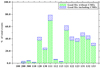 |
Fig. 1. Histogram of the GFs of the entire data set for each fitted (total) distribution fijk. The blue boxes show the additional GFs for the events during CMEs. See Table 1 for the corresponding values. |
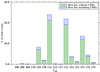 |
Fig. 2. Histogram for the BFs of the entire data set. The green boxes show the BFs without CMEs; the blue boxes show the additional BFs with CMEs. See Table 1 for the corresponding values. |
Our analysis covers the Ulysses data from the launch in late 1990 to early 2008. In total, there are 324 450 events, including 30 558 events during coronal mass ejections (CMEs), which are taken from Richardson (2014). During CMEs (reduced in number, below 10% of the number of events of a certain relevance) the electrons may exhibit a double strahl or two beaming components, sunwards and anti-sunwards, moving along the closed magnetic field topology. Thus, a double strahl (more or less symmetric) is not reproduced by our models, but it can mimic a suprathermal component with an excess of temperature anisotropy in the direction parallel to the magnetic field. To avoid such a confusing interpretation, the events during CMEs are counted separately in our present analysis. In addition, we rejected 2139 events that violated condition (2). The total number of bad fits is about 20%. Ideally, a data set consists of 400 data points with finite values, but most of the time there are much fewer such points, due to the missing data. If the number of these points is too low, the fits become unreliable, as indicated by the mean error and the standard deviation in the case of rejected fits. The data set is given in keV without any error estimates, thus we were not able to weight the data according to their observational errors, and therefore the weight is always unity.
In Fig. 1 we show the distribution of GFs for all individual distributions functions fijk. The most reduced relevance can be attributed to single fits, like f100, f200, or f300, with less than 4% of the total events, and those reproducing the halo with a Maxwellian and the strahl with GAK (f112 with GFs < 7%) or RAK (f113, with GFs < 3%); see Table 1. The highest peak is given by a standard combination of three AMDs, that is, the f111 combination, with the ability to provide GFs for about 70% of the total data (in the absence of CMEs, in green). However, GFs are also obtained with all the other combinations involving GAK or RAK for describing the suprathermal populations. These combinations dominate the histogram with representations between 20% and more than 50% of the total number of events: f130 with ∼22.5%; f133 with ∼29%, f120, f122, f123, and f132, each approaching 40%; f131 with ∼45%; and f121 with ∼54% (see Table 1).
These results are refined in Fig. 2, which shows the distribution of the BFs for the entire data set (in green for the events without CMEs). The number of BFs (in %) obtained for each combination of distribution functions is given in Table 1, and together sum up to 80.6% of the total number of events (70.7% without CMEs). Thus, each valid event is assigned one of these fitting combinations fijk. It can be seen that 21.2% of the events without CMEs are best fitted by the f111 combination. This is closely followed by f121 with 19.1%, and then by f131 with 12.1%, f120 with 7.1%, f132 with 3.8%, f122 with 3.2%, and f130 with 1.7%. Remarkably, there are dual core–halo distributions (in the absence of strahl, i.e., f120 and f130), with almost 9% of the relevant events. BFs around 1% are obtained for combinations like f123 and f133, while single distributions using GAK (i.e., f200) or RAK (i.e., f300) have a very reduced presence, with 0.3% and 0.1%, respectively. Fitting models involving generalized Kappa distributions, like GAK or RAK, total 56.7% of the events (49.5% without CMEs). It is noteworthy that 59.4% of the events (52.4% without CMEs) have the strahl component best reproduced by an AMD, while halos are described by a GAK in about 35% of the events (30.5% without CMEs), and by an RKD in about 21% of the events (18.3% without CMEs). We also note that the most prominent fit combines three AMDs, for 24% of all events (21.2% without CMEs).
In order to check if the more complicated GAK–halo distribution (f121) could be replaced by a simpler RAK–halo distribution (f131), we compare the BFs of the f121 distribution with the GFs of the f131 distribution. Figure 3 displays the mean error of the BFs of the f121 distribution against the mean error of GFs of the corresponding f131 distribution. It can be seen that about half of the f121 distributions can be replaced by the f131 distribution and still obtain a GF. In total, we have 63 821 f121 BF events, which can be replaced by 37 263 GF events of the f131 distribution. Thus, about 58% of the f121 distribution could be replaced by the f131 distribution. This can be helpful in analytic studies of dispersion relations. Nevertheless, we still have about 42% (26 558) events of the f121 distribution for which the fits of the f131 distribution give only bad results.
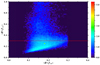 |
Fig. 3. Correlating the mean error of GFs of the f121 distribution and the mean error of GFs of the f131 distribution. The red line indicates the threshold for a GF. |
The total number of bad fits is about 19.4% or 62 843 events, together with 2139 rejected events (0.66%). These data shall be handled individually (about 20%) because the fit procedure needs to start with a different initial guess, the data sets are too spare to be fitted, or the data cannot be fitted with the above combinations of distribution functions. In the present analysis, from the total number of events we consider the remaining majority of 80%, or 259 365 events. In the following we discuss the correlation between macroscopic parameters, and concentrate only on the BFs that are unique. We mainly refer to the most representative combinations (e.g., f111, f121, and f131), although the analysis may also take into account the less prominent examples (e.g., f120, f122, or f132).
3. Time and speed variations
We recall the time and latitude dependence of the solar wind speed along the Ulysses trajectory (McComas et al. 2008), and again present in Fig. 4 the angular distribution from McComas et al. (2008). It can be seen that during the first and third latitude scan there are low solar wind speeds below ≈35° latitude and high speeds above ≈35° latitude, and almost no intermediate speeds. This is different during a more active Sun in the second scan, when the speeds scatter over all latitudes.
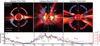 |
Fig. 4. Ulysses solar wind speeds over time, adapted from McComas (2008). The three upper panels show the solar wind proton speed as a function of heliographic latitude in a polar coordinate system, during solar minimum (upper right panel), solar maximum (upper centre panel), and again solar minimum (upper left panel). The corresponding sun spot number (solar activity) is shown in the lower panel, where the black line gives the sunspot number and the red line the tilt angle. Indicated in the lower inset are the dominant distribution functions during that period to illustrate the solar cycle dependence of the electron distribution functions shown in Fig. 6. |
The difference in solar wind speeds depending on the latitude is also evident in Fig. 5, which shows the histograms of the number of events (in %) as a function of the solar wind speed. We split the figure into a part for low latitudes < 30° (upper panel) and a part for high latitudes > 40° (lower panel). This time the events (and the corresponding values) without CMEs are given in black, while those during CMEs in blue. The gap at intermediate speeds, with about 2.5% of events, is obvious around ≈650 km s−1. These histograms also show that the low speeds cluster around 450 km s−1 at low latitudes near the ecliptic (upper panel), while the high speeds cluster around 750 km s−1 at high latitudes towards the poles and coronal holes (lower panel). Thus, high speeds are mainly observed during solar minimum (see also McGregor et al. 2011).
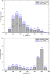 |
Fig. 5. Histograms of the number of events depending on solar wind speed during the Ulysses mission, from low latitudes < 30° (upper panel) and from high latitudes > 40° (lower panel). |
In Fig. 6 the histogram of Fig. 2 is divided into individual years. This helps us to find the combinations of distribution functions relevant for each orbit of the Ulysses missions, and implicitly for different solar activities. These combinations are also indicated in Fig. 4, in order of their relevance as follows: [f111, f121, f131, f120] for the first and third orbits, and [f121, f111, f131, f120] for the second orbit. Instead, the f111 and f131 distributions have a dip around the years 1996–2000, which is the ascending phase of solar cycle 23 (see Fig. 4), while the f121 and f122 distributions show a maximum. Unfortunately, this is the only ascending phase covered by the Ulysses mission. Therefore, we can only guess that during the ascending phases of a solar cycle, the f121 (f122) distributions are more appropriate. In two declining phases (that of solar cycles 22 and 23) the distribution functions f111 and f131 give the most relevant BFs, although f121 is also well represented in this case. Thus, in a declining phase of a solar cycle, the electron distributions are better reproduced by three Maxwellians, meaning that they are, individually, closer to thermal equilibrium. Contrarily, in the rising phase, when the solar activity increases, the halo distribution is not well fitted by Maxwellians, meaning that the particles are no longer in thermal equilibrium. The above also holds true for the period around 2002, where the f111 and f131 distributions have a minimum, and later at 2007 show a maximum (and vice versa for the f121 and f122 distributions). However, because this is at the end of the misson and no further data are available, we cannot safely conclude that this time dependence is verified by observations. The reason is that the time series only covers parts of a solar Hale cycle, but at least a few such cycles were needed. From a theoretical point of view the time dependence can be explained by the changing magnetic field in the rising phase and the beginning of the solar activity. Thus, the non-equilibrium distributions f121 (f122) can be caused by an enhanced flare activity. This proposed context needs a more detailed analysis including all spacecraft and solar data, which is far beyond the topic of this work.
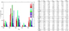 |
Fig. 6. Histogram and table of relative numbers given on a yearly basis. Left panel: histogram for the BFs of individual years. Inside a distribution function fijk each bar represents the events per year, from 1990 to 2008. The data for 2005 are missing. The data for 1990 at the beginning of the mission are very sparse, which is also the case towards the end of the mission (after 2005). Right panel: relative number of events by the BFs of the five most representative distribution functions. For each intermediate row, |

4. Case study: Temperature anisotropy
We define the four temperature anisotropies as
 (9)
(9)
and we define the parallel plasma beta as
 (10)
(10)
with magnetic field magnitude B. The β⊥ can be defined, but is not discussed here. See Appendix A for further information including the representation method in Figs. 7–10. Furthermore, we only discuss the events without CMEs, and the distributions in the CMEs will be left for future work. We display the total number of events on a multi-coloured scale, while the number of core events is displayed on a red scale, that of the halo on a blue scale, and that of the strahl on a green scale.
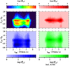 |
Fig. 7. Correlating the solar wind speed (x-axis) given in units of 100 km s−1 and the temperature anisotropy (y-axis) for all events. The number of events |

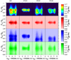 |
Fig. 8. Correlating the solar wind speed and the temperature anisotropy without CMEs. The results shown in the columns from left to right are for fall, f111, f121, and f131, respectively. Rows from top to bottom display the results for the total, core, halo, and strahl distributions, respectively. See text for more details. |
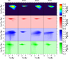 |
Fig. 9. Correlating the parallel plasma beta and the temperature anisotropy. Panels are organized as in Fig. 8. See text for more details. |
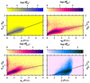 |
Fig. 10. Correlation between the temperature anisotropy and parameters of the halo components of the distributions are displayed. The temperature anisotropy is compared with the κ parameter of the f131 distribution (upper left panel), and with the η∥, η⊥, and ζ parameters of the f121 distribution (upper right panel, lower left panel, and lower right panel, respectively). For further explanation, see text. |
4.1. Temperature anisotropy and solar wind speed.
Figures 7 and 8 display the colour-coded binned number of events  (see Appendix A.1), in a plot with the solar wind speed versus the temperature anisotropy (Eq. (9)). In Fig. 7 we correlate temperature anisotropy and solar wind speeds for the total distribution function of all events (upper left panel), and only for the core (upper right panel), for the halo (lower left panel), and for the strahl (lower right panel). In the upper left panel, four maxima in the number of all events
  can be identified: the first between vsw = 300−500 km s−1 and an anisotropy of A ≈ 1, the second between vsw ≈ 700 km s−1 and vsw ≈ 800 km s−1 and A ≈ 1, and the third and fourth at about the same solar wind speeds, but at lower temperature anisotropies A ≈ 0.5. The core distribution contributes mainly to the first and second maxima (upper right panel), while the halo distribution determines the third and fourth maxima, and contributes also to the first and second maxima (lower left panel). The strahl distribution (lower right panel) contributes primarily to the first and second maxima. This implies that the temperature anisotropy is mainly caused by the halo and strahl components, while the core distribution is well fitted with an isotropic (A = 1) temperature distribution function. The dip at solar wind speeds about vsw ≈ 650 km s−1 is due to the fact that these speeds are rare (see Figs. 4 and 5).
Figure 8 is structured similarly to Fig. 7, and shows a comparison of fall with f111, f121, and f131 (from left to right) by plotting  of the corresponding total, core, halo, and strahl distributions. It can be seen that the f111 distributions have maxima at temperature anisotropies around A = 1 for all four plots: total, core, halo, and strahl. The f121 distribution has two maxima along A ≈ 1 and A ≈ 0.5, where the former is mainly the contribution from the core, while the latter are contributions from the halo and the strahl. The core of the f121 distribution has a behaviour similar to that of f111 distribution, that is, it scatters mainly around A = 1. A similar behaviour shows the f131 distribution, except that the halo does not scatter as much as the halo of the f121 distribution. In addition, the total anisotropy is smoother for the f131 distribution. The total anisotropy for the f111 distribution scatters only around A = 1 (temperature isotropy), while the total of the f121 distribution has two maxima around A = 1 and A = 0.5, similar to the f131 distributions, except that the second maximum around A = 0.5 is not very pronounced. The dips are again explained by the absence of speeds about vsw ≈ 650 km s−1 (see above).
The f121 distribution shows the strongest scattering in the halo and superhalo component. Nevertheless, because this is the BF, it indicates that there might be another distribution function involved not covered by the fitted AMD, RKD, or GAK distributions. The scattering in the fitted halo by the f121 distribution might also occur due to the general nature of the GAK. We do not make a closer inspection here, but state that the bulk of the data is in the maximum of the f121 distribution, so that the GAK can be used for fitting.
To conclude this section, we point out that the core has in this analysis a bi-Maxwellian distribution, which can be replaced by an isotropic Maxwell distribution, while the halo and superhalo/strahl are best fitted with anisotropic distributions (here an RAK or GAK). In many cases we can also replace the GAK by the RAK (see the discussion in Sect. 2).
4.2. Temperature anisotropy and parallel plasma beta
Figure 9 displays the temperature anisotropy as a function of the parallel plasma beta. In the top panel of first column the total temperature anisotropy of all events is shown. For all distributions, the core events (second row) show small deviations from isotropy and distribute regularly, approximately parallel to the x-axis. The halo events (first column, third row) predominantly show an excess of parallel temperature T‖,h > T⊥,h, revealing a mushroom-like shape, with the ‘stalk’ at β∥ ≈ 0.1, and the ‘cap’ widely ranging from very low to high values of β∥, h: 10−4 < β∥, h < 50. The strahl events (first column, fourth row) are similar, but spread at slightly lower values of β∥, s < 1. The distributions of these data are very similar to those obtained by Štverák et al. (2008) with the ecliptic electron data.
The second, third, and fourth columns of Fig. 9 display the events fitted by f111, f121, and f131, respectively. It can be seen that the f111 distribution has a very weak scattering in all components and is quite similar to the above-mentioned plots by Štverák et al. (2008). This is also true for the core events of all other distributions (second row). However, the halo events of the f121 and f131 distributions show much stronger scattering (third row). Although more constrained, the strahl component (fourth row) shows the same variation. For all distributions, the stalk is thus a feature mainly resulting from the other distributions not shown here (e.g., the f120 and f122 distributions).
4.3. Temperature anisotropy and κ, η∥, η⊥, and ζ parameters
In Fig. 10 we show the correlation between parameters of the halo components of the f131 and f121 distributions with the temperature anisotropy. The color-coding is given at the top of each panel. In the upper left panel the scattering of the κ values of the f131 distribution is shown. We can see that κ has only values between 0 and about 2.5. It is also evident that the lower the κ values, the lower the halo temperature anisotropy; in other words, the perpendicular temperature is much higher than the parallel temperature. The reason for κ values only below 2.5 can be due to the fact that for higher κ values the distribution is comparable to a Maxwellian, and thus the distribution f121 approaches f111. However, this statement requires more research.
For the f121 distribution, the scattering of the η∥, η⊥, and ζ parameters is similar to the scattering of the κ values in the f121 distribution, except that η∥ has higher values (up to 5, see upper right panel), while the η⊥ values are in a range similar to that of κ (left lower panel). The ζ parameter (right lower panel) is similar to the η⊥ parameter. The f131 halo component also shows an increased scattering in the anisotropy around η∥ = 0, η⊥ = 0, and ζ = 0, which can be caused by the fitting procedure due to the small values of the corresponding parameters.
We computed a linear regression for the data shown in Fig. 10 via
 (11)
(11)
where x ∈ {κ, η∥, η⊥, ζ}. The values for the fits are listed in Table 2. The linear regression is quite good for A(κ), but for A(η∥) and A(η⊥) the events form a curve asymptotically approaching A = 1. The fit for A(ζ) runs through a cloud, which clusters around the linear regression and scatters towards higher anisotropies. Nevertheless, the simplified regressions can help us to study the temperature anisotropy in the halo with increasing values of κ, η∥, η⊥, and ζ.
5. Conclusions
In the present work we used a 2D fitting method, which accounts for different temperatures, parallel and perpendicular with respect to the background magnetic field, to fit the electron velocity distributions obtained during the Ulysses mission. In doing so, we used a triple model to fit the core, halo, and superhalo/strahl populations within the total distribution. As model functions we applied an anisotropic Maxwellian distribution (AMD), a generalized anisotropic Kappa (GAK), and a regularized anisotropic Kappa (RAK) distribution. Our findings indicate a time dependence of the electron distributions on the solar cycle. Unfortunately, the data series is not long enough to solidly confirm this behaviour. Nevertheless, the results suggest that in a declining phase of a solar cycle, the individual electron distributions are best described by three Maxwellians, meaning that they are in thermal equilibrium. In the ascending phase, when the solar activity increases, the halo distribution is not well fitted by a Maxwellian, which means that the particles are out of thermal equilibrium. This behaviour deserves more attention and should be combined with other spacecraft data. However, due to the unique solar polar orbit of Ulysses and that most of the other spacecraft are in the ecliptic (HELIOS) or close to the Sun (Parker Space Probe, Solar Orbiter), in principle the distance and latitude effects need to be subtracted.
While the core distribution can most likely be fitted with an isotropic Maxwell distribution as the temperature anisotropy is close to 1 (see the red panels in the figures in Sect. 4), the halo and superhalo/strahl (the blue and green panels) are best fitted with anisotropic distributions (here with an RAK or a GAK). In many cases we can also replace the GAK by the simpler RAK, resulting in a slightly worse fit (see Fig. 3).
The parallel plasma beta correlation with the temperature anisotropy is similar for the three distributions f111, f121, and f131, but shows a stalk for the halo distribution in the sample of all distributions. We also showed the correlation between the temperature anisotropy and the κ parameter of the f131 distribution as well as the η∥, η⊥ and ζ parameters of the f121 distribution. The temperature anisotropy shows almost a linear dependence on κ with increasing values of κ, and the temperature anisotropy becomes more isotropic. For the GAK parameters (η∥, η⊥, ζ) we also found a linear dependence of the temperature anisotropy.
Finally, we would like to highlight Fig. 4, which shows that during a solar cycle the type of distribution function changes from mainly a f111 type near solar minimum to a more general f121 type close to solar maximum, and then goes back to f111 for the next minimum phase. These results demonstrate that the multi-distribution function fitting of velocity distributions has a significant potential to advance our understanding of the solar wind kinetics and, therefore, deserves further quantitative analyses.
The data sets were derived from sources in the public domain2.
Acknowledgments
The authors acknowledge support from the Ruhr-University Bochum and the Katholieke Universiteit Leuven. EH is grateful to the Space Weather Awareness Training Network (SWATNet) funded by the European Union’s Horizon 2020 research and innovation programme under the Marie Skłodowska-Curie grant agreement No 955620. ML acknowledges support in the framework of the project SIDC Data Exploitation (ESA Prodex-12).
References
- Alexandrova, O., Chen, C. H. K., Sorriso-Valvo, L., Horbury, T. S., & Bale, S. D. 2013, Space Sci. Rev., 178, 101 [Google Scholar]
- Bale, S. D., Kasper, J. C., Howes, G. G., et al. 2009, Phys. Rev. Lett., 103, 211101 [NASA ADS] [CrossRef] [Google Scholar]
- Bame, S. J., McComas, D. J., Barraclough, B. L., et al. 1992, A&AS, 92, 237 [NASA ADS] [Google Scholar]
- Kasper, J. C., Lazarus, A. J., Steinberg, J. T., Ogilvie, K. W., & Szabo, A. 2006, J. Geophys. Res., 111, A03105 [NASA ADS] [CrossRef] [Google Scholar]
- Lazar, M. 2012, Exploring the Solar Wind (Rijeka: Intech Europe) [CrossRef] [Google Scholar]
- Lazar, M., & Fichtner, H. 2021, Kappa Distributions: From Observational Evidences via Controversial Predictions to a Consistent Theory of Non-equilibrium Plasmas (Berlin: Springer) [CrossRef] [Google Scholar]
- Lazar, M., Pomoell, J., Poedts, S., Dumitrache, C., & Popescu, N. A. 2014, Sol. Phys., 289, 4239 [NASA ADS] [CrossRef] [Google Scholar]
- Lazar, M., Pierrard, V., Shaaban, S. M., Fichtner, H., & Poedts, S. 2017, A&A, 602, A44 [NASA ADS] [CrossRef] [EDP Sciences] [Google Scholar]
- Lin, R. P. 1998, Space Sci. Rev., 86, 61 [NASA ADS] [CrossRef] [Google Scholar]
- Macneil, A. R., Owen, M. J., Lockwood, M., Štverák, Š., & Owen, C. J. 2020, Sol. Phys., 295, 16 [NASA ADS] [CrossRef] [Google Scholar]
- Maksimovic, M., Pierrard, V., & Riley, P. 1997, Geophys. Rev. Lett., 24, 1151 [NASA ADS] [CrossRef] [Google Scholar]
- Maksimovic, M., Zouganelis, I., Chaufray, J.-Y., et al. 2005, J. Geophys. Res. (Space Phys.), 110, A09104 [NASA ADS] [CrossRef] [Google Scholar]
- Marsch, E. 2006, Liv. Rev. Sol. Phys., 3, 1 [Google Scholar]
- Mason, G. M., & Gloeckler, G. 2012, Space Sci. Rev., 172, 241 [NASA ADS] [CrossRef] [Google Scholar]
- McComas, D. J. 2008, Space Sci. Rev., 122 [Google Scholar]
- McComas, D. J., Ebert, R. W., Elliott, H. A., et al. 2008, Geophys. Rev. Lett., 35, 18103 [NASA ADS] [CrossRef] [Google Scholar]
- McGregor, S. L., Hughes, W. J., Arge, C. N., Owens, M. J., & Odstrcil, D. 2011, J. Geophys. Res. (Space Phys.), 116, A03101 [NASA ADS] [Google Scholar]
- Olbert, S. 1968, in Physics of the Magnetosphere, eds. R. D. L. Carovillano, & J. F. McClay, Astrophys. Space Sci. Lib., 10, 641 [NASA ADS] [CrossRef] [Google Scholar]
- Paschmann, G., Fazakerley, A. N., & Schwartz, S. J. 1998, ISSI Sci. Rep. Ser., 1, 125 [NASA ADS] [Google Scholar]
- Pierrard, V., Maksimovic, M., & Lemaire, J. 2001, Astrophys. Space Sci., 277, 195 [NASA ADS] [CrossRef] [Google Scholar]
- Pilipp, W. G., Miggenrieder, H., Montgomery, M. D., et al. 1987a, J. Geophys. Res.: Space Phys., 92, 1075 [NASA ADS] [CrossRef] [Google Scholar]
- Pilipp, W. G., Miggenrieder, H., Montgomery, M. D., et al. 1987b, J. Geophys. Res.: Space Phys., 92, 1093 [NASA ADS] [CrossRef] [Google Scholar]
- Pilipp, W. G., Miggenrieder, H., Mühlhäuser, K. H., et al. 1987c, J. Geophys. Res.: Space Phys., 92, 1103 [NASA ADS] [CrossRef] [Google Scholar]
- Richardson, I. G. 2014, Sol. Phys., 289, 3843 [NASA ADS] [CrossRef] [Google Scholar]
- Scherer, K., Fichtner, H., & Lazar, M. 2017, Europhys. Lett., 120, 50002 [NASA ADS] [CrossRef] [Google Scholar]
- Scherer, K., Lazar, M., Husidic, E., & Fichtner, H. 2019, ApJ, 880, 118 [NASA ADS] [CrossRef] [Google Scholar]
- Scherer, K., Husidic, E., Lazar, M., & Fichtner, H. 2020, MNRAS, 497, 1738 [NASA ADS] [CrossRef] [Google Scholar]
- Scherer, K., Husidic, E., Lazar, M., & Fichtner, H. 2021, MNRAS, 501, 606 [Google Scholar]
- Štverák, Š., Trávníček, P., Maksimovic, M., et al. 2008, J. Geophys. Res.: Space Phys., 113, A03103 [Google Scholar]
- Vasyliunas, V. M. 1968, in Physics of the Magnetosphere, eds. R. D. L. Carovillano, & J. F. McClay, Astrophys. Space Sci. Lib., 10, 622 [NASA ADS] [CrossRef] [Google Scholar]
- Wilson, L. B., Chen, L.-J., Wang, S., et al. 2019a, ApJS, 243, 8 [NASA ADS] [CrossRef] [Google Scholar]
- Wilson, L. B., Chen, L.-J., Wang, S., et al. 2019b, ApJS, 245, 24 [NASA ADS] [CrossRef] [Google Scholar]
- Wilson, L. B., Chen, L.-J., Wang, S., et al. 2020, ApJ, 893, 22 [NASA ADS] [CrossRef] [Google Scholar]
- Yoon, P. H. 2011, Phys. Plasmas, 18, 122303 [NASA ADS] [CrossRef] [Google Scholar]
- Yoon, P. H., Ziebell, L. F., Gaelzer, R., Wang, L., & Lin, R. P. 2013, Terr. Atmos. Ocean Sci., 24, 175 [CrossRef] [Google Scholar]
Appendix A: Pressure and temperature moments
We briefly repeat here the definitions given in Paschmann et al. (1998) and Scherer et al. (2021). The partial parallel and perpendicular thermal pressures are as follows:
 (A.1)
(A.1)
The total pressure Ptot is the sum of the thermal pressure plus (twice) the ram pressure (see Scherer et al. 2021 for further explanation).
The respective temperatures are given by the ideal gas law as
 (A.2)
(A.2)
with kB denoting Boltzmann’s constant, and
 (A.3)
(A.3)
where the number density nt is given by
 (A.4)
(A.4)
A.1. Representation method
In the graphical representations we divide the x- and y-axis into 100 sub-intervals Δxi and Δyj, and compute the total number of events (data points) Nall in each interval Ni, j/(ΔxiΔyj) via
 (A.5)
(A.5)
As stated above, we only discuss the macroscopic parameters for the most relevant distribution functions, according to their BFs, that is fall, f111, f121, and f131, where fall are all the BFs including all distributions fijk. We always show the total first, and then core, halo, and superhalo/strahl moments for fall, and then we show how the moments for the single distributions f111, f121, and f131 contribute to fall.
All Tables
All Figures
|
Fig. 1. Histogram of the GFs of the entire data set for each fitted (total) distribution fijk. The blue boxes show the additional GFs for the events during CMEs. See Table 1 for the corresponding values. |
| In the text | |
|
Fig. 2. Histogram for the BFs of the entire data set. The green boxes show the BFs without CMEs; the blue boxes show the additional BFs with CMEs. See Table 1 for the corresponding values. |
| In the text | |
|
Fig. 3. Correlating the mean error of GFs of the f121 distribution and the mean error of GFs of the f131 distribution. The red line indicates the threshold for a GF. |
| In the text | |
|
Fig. 4. Ulysses solar wind speeds over time, adapted from McComas (2008). The three upper panels show the solar wind proton speed as a function of heliographic latitude in a polar coordinate system, during solar minimum (upper right panel), solar maximum (upper centre panel), and again solar minimum (upper left panel). The corresponding sun spot number (solar activity) is shown in the lower panel, where the black line gives the sunspot number and the red line the tilt angle. Indicated in the lower inset are the dominant distribution functions during that period to illustrate the solar cycle dependence of the electron distribution functions shown in Fig. 6. |
| In the text | |
|
Fig. 5. Histograms of the number of events depending on solar wind speed during the Ulysses mission, from low latitudes < 30° (upper panel) and from high latitudes > 40° (lower panel). |
| In the text | |
|
Fig. 6. Histogram and table of relative numbers given on a yearly basis. Left panel: histogram for the BFs of individual years. Inside a distribution function fijk each bar represents the events per year, from 1990 to 2008. The data for 2005 are missing. The data for 1990 at the beginning of the mission are very sparse, which is also the case towards the end of the mission (after 2005). Right panel: relative number of events by the BFs of the five most representative distribution functions. For each intermediate row, |
| In the text | |
|
Fig. 7. Correlating the solar wind speed (x-axis) given in units of 100 km s−1 and the temperature anisotropy (y-axis) for all events. The number of events |
| In the text | |
|
Fig. 8. Correlating the solar wind speed and the temperature anisotropy without CMEs. The results shown in the columns from left to right are for fall, f111, f121, and f131, respectively. Rows from top to bottom display the results for the total, core, halo, and strahl distributions, respectively. See text for more details. |
| In the text | |
|
Fig. 9. Correlating the parallel plasma beta and the temperature anisotropy. Panels are organized as in Fig. 8. See text for more details. |
| In the text | |
|
Fig. 10. Correlation between the temperature anisotropy and parameters of the halo components of the distributions are displayed. The temperature anisotropy is compared with the κ parameter of the f131 distribution (upper left panel), and with the η∥, η⊥, and ζ parameters of the f121 distribution (upper right panel, lower left panel, and lower right panel, respectively). For further explanation, see text. |
| In the text | |
Current usage metrics show cumulative count of Article Views (full-text article views including HTML views, PDF and ePub downloads, according to the available data) and Abstracts Views on Vision4Press platform.
Data correspond to usage on the plateform after 2015. The current usage metrics is available 48-96 hours after online publication and is updated daily on week days.
Initial download of the metrics may take a while.