© ESO, 2022

1 Introduction

Small fragments of comets and asteroids of sizes ranging from micrometres (μm) to millimetres (mm) moving in various orbits around the Sun remain unexplored for most of the time. Over a long period of time, the initial orbits of these dust particles, known as meteoroids, change due to interactions with other planets or non-gravitational forces, or both. As a result, a small fraction of the meteoroid population will inevitably encounter the orbits of planets with an atmosphere and produce meteors or meteor showers. Detailed measurements of their dynamic behaviour and properties during their atmospheric entry can be used for the geometric reconstruction of their trajectories and the subsequent determination of their heliocentric orbits.

A number of different methods for the trajectory determination using optical systems have been developed over recent years. The two most well-established approaches are the plane-intersection method described by Ceplecha (1987) and the straight line least squares (SLLS) method published by Borovicka (1990). The plane intersection method fits a 2D plane from line-of-sight (LoS) measurements for each station. The trajectory of a meteor is then calculated by intersecting the planes generated from at least two stations in space. In the present paper, we refer to this travelled path by a meteor as the trajectory line. In the case of multi-station observations, the best trajectory is calculated as the average line considering the geometry between each individual trajectory solution. On the other hand, the SLLS method provides a least squares solution for the trajectory line by minimising the sum of the squared orthogonal distances of all measured direction vectors to the meteor line in space. Even though the latter approach allows each LoS measurement to influence the solution, measurements from a single station are given the same weight depending solely on the station-meteor geometry. Uncertainties of single measurements have an impact on the determined trajectory and must therefore be taken into account. This problem becomes evident when measurements provided by several camera systems with different characteristics (e.g. resolution, optics, etc.) are used for the estimation of the trajectory.

Recently, several authors noted the need to consider the standard deviations of measurements in the computation of the meteor trajectory (Gural 2012; Sansom et al. 2019; Vida et al. 2020). In the study by Vida et al. (2020), the estimated errors of the measurements contribute to the trajectory solution as follows: first an estimate of the trajectory line is computed by applying the plane-intersection method, which is later used as starting values for the iterative procedure of the SLLS method. By introducing Gaussian noise to the original measurements with standard deviations based on the errors of the first trajectory estimation, a new solution is calculated. This iterative process continues until the solution converges, indicating the best fit, considering dynamic and geometric parameters of the meteoroid.

Jeanne et al. (2019) presented a data reduction pipeline which they applied to image data acquired by the Fireball Recovery and InterPlanetary Observation Network (FRIPON) (Colas et al. 2012). Similarly to previous studies, estimation of the meteor trajectory is based on the SLLS method. An empirical weight was introduced for each camera system modifying the objective function to be minimised under the assumption that systematic errors, characterised by imperfections present at each station, dominate the measurement errors on the images. As a result, the different characteristics of each camera system can be taken into account when computing the trajectory of a meteor observed from multiple stations.

Gural (2012) presented a solution for the determination of the trajectory line of a meteoroid, which incorporates the dynamic behaviour of the motion of the body. The initial velocity, that is the velocity before any deceleration occurs, the deceleration parameters, and the position of the meteoroid during its atmospheric entry are determined by means of a least squares adjustment. This solution strategy assumes that identical characteristics of the meteoroid will be observed from different camera systems, allowing the computation of possible time-offsets between stations due to synchronisation deficiencies. Empirical errors are estimated for the unknown parameters of the model in terms of Monte Carlo simulations. This approach has been used by several authors (Jenniskens et al. 2011; Vida et al. 2020) and was extended by Egal et al. (2017) by implementing various optimisation techniques for solving the minimisation problem.

The camera systems of the Desert Fireball Network (DFN) are able to register a meteor event with submillisecond precision allowing point-to-point triangulations of multi-station observations (Howie et al. 2017; Sansom et al. 2019). High temporal resolution is achieved using a liquid crystal shutter which generates a unique pattern of short and long pulse widths along the meteor trail. The pattern is then decoded to binary elements (0,1) corresponding to a specific time interval within a single exposure. Each camera station is equipped with a GNSS receiver which provides absolute timing for every recorded meteor event. Sansom et al. (2017) presented a sequential Monte Carlo solution incorporating dynamical as well as physical parameters to the trajectory solution of the meteor in three dimensions.

In the studies of Ceplecha (1987) and Borovicka (1990), the standard deviations of the LoS measurements were, in some sense, disregarded and the stochastic model is based solely on the geometry between each station and the meteor. In the most recent studies, a combined solution for the 3D motion of the meteoroid is provided, including velocity and deceleration parameters in a single step. In these cases, the standard deviations of the measurements are empirically assigned using Monte Carlo simulations.

In the present paper, we propose a new geometrical approach for fitting a straight line to multi-station LoS measurements inspired by the solution of Borovicka (1990). Our goal is to take into account the stochastic information of the LoS measurements and the geometry between each station and the recorded meteor, resulting to a more realistic stochastic model. The newly presented solution strategy for the discussed problem is based on the development of a new functional model, where the LoS measurements are treated as observations. The inclusion of more general stochastic models allows weights to be computed individually or as a combination of (a) the precision of the observed LoS measurements and (b) the geometrical configuration between each station and the recorded meteor.

Only overdetermined configurations are considered, where the solution for the searched parameters is determined by means of a least squares adjustment. For the considered case of trajectory determination, this leads to a non-linear adjustment problem with condition equations and general weights for the observations. We therefore present a least squares solution based on the Gauss-Newton approach. Such a solution can be determined by an iteratively linearised Gauss-Helmert (GH) model, as shown in (Ghilani 2018, p. 497 ff.), (Niemeier 2008, p. 172 ff.), or (Perovic 2005, p. 203). Furthermore, we avoid the pitfalls mentioned by Pope (1972) and Lenzmann & Lenzmann (2004) when dealing with the linearisation of non-linear adjustment problems.

The paper is organised in four sections: Sect. 2 describes the main objective of this work and presents current approaches for estimating meteor trajectories. Section 3 presents a detailed description of the new approach including the mathematical formulae for the adjustment solution. In Sect. 4 we describe a numerical example and present the results of the trajectory solution by means of two different methods. Finally, in Sect. 5 we summarise the results presented in the previous section and draw conclusions.

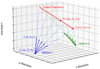Fig. 1 Schematic illustration of the observation of a linear trajectory from two locations.

2 Existing approaches for estimation of a 3D linear trajectory

In this section, we give a short overview of the two predominant approaches in the literature for estimating a 3D linear trajectory of a body, in particular the parameters of a spatial straight line.

2.1 Problem definition

Let us assume a meteoroid observed from a station P_S (X_S, Y_S, Z_S) in a 3D Cartesian coordinate system. The relationship between an image plane and the 3D space can be mathematically established by performing a geometric calibration of the camera system that acquired the image. Hence, from the measured pixel positions of a meteortrailin the image plane, the direction vectors V_i(a_i, b_i, c_i) and their standard deviations can be derived, with i = 1,…,n and n being the number of measurements from a station. The components a_i, b_i, and c_i; can be seen as the coordinate difference of a point on each direction vector and the point of the station P_S. An illustration of the problem using two stations is presented in Fig. 1.

In this study, we assume that the body is moving on a linear trajectory, that is, a spatial straight line. This assumption was found to be valid for meteors observed by commercial all-sky camera systems, because any deceleration cannot be measured (Jeanne et al. 2019). The goal is to estimate the direction of the line in which the body moves, a point on that line, and their uncertainties. The equation of a line passing through a point on the body's trajectory P_M (X_M, Y_M, Z_M) parallel to a direction vector V_M(a_M, b_M, c_M) can be described by $$\frac{X-X_{\text{M}}}{a_{\text{M}}}=\frac{Y-Y_{\text{M}}}{b_{\text{M}}}=\frac{Z-Z_{\text{M}}}{c_{\text{M}}},$$(1)

with X, Y, and Z denoting any point on this line, as shown in (Bronshtein et al. 2007, p. 217). The components a_M, b_M, and c_M can be seen as the coordinate difference of a point on the direction vector of the body’s trajectory and the point on the observed body P_M. Therefore, the trajectory line of a meteor can be obtained by computing, for example, the point coordinates X_M, Y_M, and Z_M and the components a_M, b_M, and c_M of the direction vector.

In the following, we give a short overview of two existing adjustment approaches for the discussed problem, which take into account different overdetermined configurations for a least squares solution.

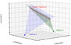Fig. 2 Geometric representation of the solution estimated by the plane intersection method from two stations.

2.2 Linear trajectory from plane intersection

Ceplecha (1987) was the first to address the discussed adjustment problem, by fitting planes to the direction vectors of each station using the method of least squares. The requested parameters of the trajectory line and point can then be computed by finding the intersection line of the two planes, as is depicted in Fig. 2.

A plane in 3D can be expressed by the general equation $$n_{x}X+n_{y}Y+n_{z}Z+d=0,$$(2)

with X, Y, and Z being the 3D coordinates of a point that lies in the plane; see Bronshtein et al. (2007, p. 214). The plane parameters are denoted with n_x, n_y, n_z, and d. Ceplecha (1987) presented a direct solution for fitting a plane to the observed direction vectors, where all vector components are taken as observations subject to random errors. This leads to the condition equations $$n_x\left(a_i-e_{a_i}\right)+n_y\left(b_i-e_{b_i}\right)+n_z\left(c_i-e_{c_i}\right)+d=0,$$(3)

with the constraint $$n_x^2+n_y^2+n_z^2=1,$$(4)

allowing all planes in space to be computed. For equally weighted and uncorrelated observations, a least squares solution can be derived by minimising the objective function $$\text{Ω}={\displaystyle \sum _{i=1}^n{e}_{a_i}^2}+e_{b_i}^2+e_{c_i}^2.$$(5)

A direct least squares solution for this non-linear adjustment is possible, as presented by Ceplecha (1987). A discussion of this adjustment problem in the context of total least squares adjustment, taking into account more general weighting cases, is provided by Malissiovas et al. (2016) and Malissiovas (2019, pp. 78–81, 113–118).

2.2.1 Linear solution for fitting a plane in 3D

Here it is important to point out that Vida et al. (2020) presented an approximate linear solution of the problem, assuming-contrary to assumptions made by Ceplecha (1987) – that coordinates in x and y directions are free of errors, leading to the linear observation equations $$c_i-e_{ci}=n_x{a}_i+n_y{b}_i+d,$$(6)

after taking into account the constraint¹ $$n_z=1.$$(7)

The solution of the approximate substitute problem can be obtained by minimising the sum of squared errors only in the z-direction $$\text{Ω}={\displaystyle \sum _{i=1}^n{e}_{c_i}^2},$$(8)

which leads to linear normal equations that can be solved directly, that is without linearisation and iterative computation, using the rules of linear algebra. This solution clearly refers to a different adjustment problem, as only the errors of the coordinates in the z-direction are taken into account and will lead to a different solution forthe plane parameters from that presented in the previous subsection.

2.2.2 Line of intersection of two planes in 3D

If the body has been observed from two stations, then two planes have to be computed in total. The trajectory line of the body is simultaneously the line of intersection of the two planes and can be computed, for example, by taking the cross product of the two planes $$V_{\text{M}}\left(a_{\text{M}},b_{\text{M}},c_{\text{M}}\right)=V_1\left(n_{x_1},n_{y_1},n_{z_1}\right)\times V_2\left(n_{x{}_2},n_{y_2},n_{z_2}\right).$$(9)

Additionally, a point on the linear trajectory P_M (X_M, Y_M, Z_M) can be obtained by computing the intersection point of one direction vector from one station to the plane of the second. For the interested reader, the equations for intersection of lines and planes can be found in Bronshtein et al. (2007, p. 218).

In the case where the body has been observed from multiple stations, then the weighted mean of all the lines of intersection can give the solution of the trajectory. This was described in detail by Ceplecha (1987) and by Vida et al. (2020).

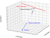Fig. 3 Simplified geometric representation of the SLLS method.

2.3 Least squares estimation of a linear trajectory

Borovicka (1990) presented an elegant geometrical way to express this adjustment problem, by taking into account each individual observed direction from multiple stations. In that study, a least squares solution was derived for the requested trajectory line by minimising the sum of squared orthogonal distances between the line described by each measured direction vector and the trajectory line. An illustration of this geometric arrangement is shown in Fig. 3.

2.3.1 Functional model and resulting observation equations

The equation of a line passing through a station P_S (X_s, Y_s, Z_s), with a direction vector V_i;(a_i, b_i, c_i), towards the observed body can be described by $$\frac{X-X_S}{a_{\text{i}}}=\frac{Y-Y_S}{b_{\text{i}}}=\frac{Z-Z_S}{c_{\text{i}}},$$(10)

with i = 1, …n and n being the number of direction vectors. The orthogonal distances between the lines of the measured direction vectors and the trajectory line Eq. (1) can be expressed by $$\begin{array}{lll}{D}_i\hfill & =\hfill & \frac{\left[\left(X_{\text{M}}-X_{\text{S}}\right)\left(b_{\text{M}}{c}_{\text{i}}-c_{\text{M}}{b}_{\text{i}}\right)\right]}{\sqrt{\left[{\left(b_{\text{M}}{c}_{\text{i}}-c_{\text{M}}{b}_{\text{i}}\right)}^2+{\left(a_{\text{M}}{c}_{\text{i}}-c_{\text{M}}{a}_{\text{i}}\right)}^2+{\left(a_{\text{M}}{b}_{\text{i}}-b_{\text{M}}{a}_{\text{i}}\right)}^2\right]}}\hfill \\ \hfill & \hfill & -\frac{\left[\left(Y_{\text{M}}-Y_{\text{S}}\right)\left(a_{\text{M}}{c}_{\text{i}}-c_{\text{M}}{a}_{\text{i}}\right)\right]}{\sqrt{\left[{\left(b_{\text{M}}{c}_{\text{i}}-c_{\text{M}}{b}_{\text{i}}\right)}^2+{\left(a_{\text{M}}{c}_{\text{i}}-c_{\text{M}}{a}_{\text{i}}\right)}^2+{\left(a_{\text{M}}{b}_{\text{i}}-b_{\text{M}}{a}_{\text{i}}\right)}^2\right]}}\hfill \\ \hfill & \hfill & +\frac{\left[\left(Z_{\text{M}}-Z_{\text{S}}\right)\left(a_{\text{M}}{b}_{\text{i}}-b_{\text{M}}{a}_{\text{i}}\right)\right]}{\sqrt{\left[{\left(b_{\text{M}}{c}_{\text{i}}-c_{\text{M}}{b}_{\text{i}}\right)}^2+{\left(a_{\text{M}}{c}_{\text{i}}-c_{\text{M}}{a}_{\text{i}}\right)}^2+{\left(a_{\text{M}}{b}_{\text{i}}-b_{\text{M}}{a}_{\text{i}}\right)}^2\right]}}.\hfill \end{array}$$(11)

Utilizing a concept of ‘zero’ observations subject to random errors expressed as the orthogonal distances D_i, Borovicka (1990) presumed the overdetermined system Eq. (11) to be nonlinear observation equations of an adjustment problem. In this case, the unknown parameters are: the coordinates of a point on the meteor X_M, Y_M, and Z_M; and the components a_M, b_M, and c_M of the direction vector parallel to the meteor, while the coordinates of each station X_S, Y_S, and Z_S and the components a_i, b_i, and C_i of the direction vectors from each station to the recorded meteor are taken as fixed values.

Therefore, the orthogonal distances Eq. (11) can be written equivalently with the general formulation $$L-\text{e}=\Phi \left(X\right),$$(12)

with the observation vector L listing only zero values and the accompanied error vector e holding the orthogonal distances D_i. The formal vector Φ holds the non-linear functional relationship between the unknown parameters, which are listed in vector $$X={\left[X_{\text{M}},Y_{\text{M}},Z_{\text{M}},a_{\text{M}},b_{\text{M}},c_{\text{M}}\right]}^{\text{T}}.$$(13)

As already explained by Borovicka (1990), it is possible to fix two unknown parameters, for example by setting $X_{\text{M}}=X_{\text{M}}^0$ and a_M = 1, with the superscript ‘0’ denoting the starting value. It is worth noting that setting parameter a_M = 1 prevents the calculation of all lines in space. For a more general solution, the constraint $a_{\text{M}}^2+b_{\text{M}}^2+c_{\text{M}}^2=1$ should be taken into account. Subsequently, the vector of unknown parameters becomes $$X={\left[Y_{\text{M}},Z_{\text{M}},b_{\text{M}},c_{\text{M}}\right]}^{\text{T}}.$$(14)

2.3.2 Stochastic model

For normally distributed errors,$e\sim \left(0,{\sigma }_0^2{Q}_{\text{LL}}\right)$, where ${\sigma }_0^2$, is the theoretical variance of the unit weight, we can construct the diagonal cofactor matrix $$Q_{\text{LL}}=\frac{1}{{\sigma }_0^2}\left[\begin{array}{llll}{\Sigma }_{{\text{LL}}_1}\hfill & 0\hfill & \cdots \hfill & 0\hfill \\ 0\hfill & \Sigma {\text{LL}}_2\hfill & \cdots \hfill & 0\hfill \\ ⋮\hfill & ⋮\hfill & \ddots \hfill & ⋮\hfill \\ 0\hfill & 0\hfill & \cdots \hfill & {\Sigma }_{\text{LL}m}\hfill \end{array}\right],$$(15)

with the diagonal variance-covariance matrices (VCMs) ${\Sigma }_{{\text{LL}}_1}$, ${\Sigma }_{{\text{LL}}_2}$, and ${\Sigma }_{{\text{LL}}_{\text{m}}}$ listing the variances of the observations for each station, and m being the number of all stations. For example, if the standard deviations of the observations were known, which is not the case in this adjustment approach, the VCM for the first station would be $${\Sigma }_{{\text{LL}}_1}=\left[\begin{array}{llll}{\sigma }_1^2\hfill & 0\hfill & \cdots \hfill & 0\hfill \\ 0\hfill & {\sigma }_1^2\hfill & \cdots \hfill & 0\hfill \\ ⋮\hfill & ⋮\hfill & \ddots \hfill & ⋮\hfill \\ 0\hfill & 0\hfill & \cdots \hfill & {\sigma }_1^2\hfill \end{array}\right],$$(16)

with σ₁ being the standard deviation for the observations of the first station. Assuming a non-singular cofactor matrix, the weight matrix can be obtained from $$P=Q_{\text{LL}}^{-1}.$$(17)

As the direction vectors V_i;(a_i,b_i,c_i) are introduced as fixed (error-free) values in this adjustment approach, their precision measures cannot be taken into account in the stochastic model. Instead, Borovicka (1990) considers a different weighting concept that depends on the geometry between each station and the trajectory line. Following Vida et al. (2020), the weights are calculated as $$\begin{array}{l}{P}_{{\text{a}}_i}=\arccos \left(V_{\text{M}}\cdot V_i\right),\hfill \\ w_i={\sin }^2{P}_{\text{a}i},\hfill \end{array}$$(18)

where V_M is the computed direction vector of the trajectory line given in Eq. (9) and P_a is the perspective angle computed as the dot product between each direction vector V_i and V_M. Weights w_i are calculated for all available direction vectors of a station. Of all direction vectors V_i, the one closest to the meteor trajectory is chosen, yielding the highest weight. This occurs when a meteor is moving in a line perpendicular to the direction vector, for instance when the perspective angle is P_a = 90°. Subsequently, the computed weights from Eq. (18) can be directly introduced into the weight matrix for the first station as follows $$P_1=\left[\begin{array}{llll}{w}_1\hfill & 0\hfill & \cdots \hfill & 0\hfill \\ 0\hfill & w_1\hfill & \cdots \hfill & 0\hfill \\ ⋮\hfill & ⋮\hfill & \ddots \hfill & ⋮\hfill \\ 0\hfill & 0\hfill & \cdots \hfill & w_1\hfill \end{array}\right].$$(19)

The weight matrices P₁, P₂, P_m containing the weights for each station can be included in the weight matrix P, which yields $$P=\left[\begin{array}{llll}{P}_1\hfill & 0\hfill & \cdots \hfill & 0\hfill \\ 0\hfill & P_2\hfill & \cdots \hfill & 0\hfill \\ ⋮\hfill & ⋮\hfill & \ddots \hfill & ⋮\hfill \\ 0\hfill & 0\hfill & \cdots \hfill & P_m\hfill \end{array}\right].$$(20)

2.3.3 Least squares solution within the Gauss-Markov model

A least squares solution within the Gauss-Markov (GM) model can be derived following the Gauss-Newton approach, that is by linearising the non-linear functional model in Eq. (11) and obtaining an iterative solution for the unknown parameters by minimizing the objective function $$\text{Ω}\left(e\right)=e^{\text{T}}Pe.$$(21)

Detailed explanations of this iterative procedure are given by, for example, Niemeier (2008, p. 137 ff.) and Ghilani (2018, p.207 ff.).

2.4 Discussion and open questions

In this section we review two of the most popular approaches for the estimation of linear trajectories. These are the line of intersection of planes from Ceplecha (1987) and the SLLS from Borovicka (1990). This leads us to two open questions:

• Is there a different geometrical approach that can lead to an adjustment problem that directly involves the measured direction vectors from multiple stations?

• Is it possible to incorporate more realistic stochastic models in the adjustment, where the standard deviations of the measured direction vectors would be used directly?

3 A new approach for the determination of linear trajectories

Inspired by the solution of Borovicka (1990), in this section we present a new geometric point of view for the problem being discussed. This leads to an adjustment model that allows the inclusion of the stochastic parameters of the observed direction vectors directly.

The idea is based on the fact that the direction vectors from each station should be coplanar and not parallel to the direction of the meteor. Individual planes would describe the coplanarity between each individual station with the observed meteor, as illustrated in Fig. 4.

Two vectors or lines in space would be on the same plane if they cross each other, that is, they would not be skewed and not parallel. According to Bronshtein et al. (2007, p. 218), the determinant of the two vectors should be equal to zero, which yields $$\left|\begin{array}{ccc}\left(X_{\text{M}}-X_{\text{S}}\right)& \left(Y_{\text{M}}-Y_{\text{S}}\right)& \left(Z_{\text{M}}-Z_{\text{S}}\right)\\ a_{\text{M}}& b_{\text{M}}& c_{\text{M}}\\ a_{\text{i}}& b_{\text{i}}& c_{\text{i}}\end{array}\right|=0,$$(22)

which can be described equivalently by $$\begin{array}{c}\left(X_{\text{M}}-X_{\text{S}}\right)\left|\begin{array}{cc}{b}_{\text{M}}& c_{\text{M}}\\ b_{\text{i}}& c_{\text{i}}\end{array}\right|-\left(Y_{\text{M}}-Y_{\text{S}}\right)\left|\begin{array}{cc}{a}_{\text{M}}& c_{\text{M}}\\ a_{\text{i}}& c_{\text{i}}\end{array}\right|\\ +\left(Z_{\text{M}}-Z_{\text{S}}\right)\left|\begin{array}{cc}{a}_{\text{M}}& b_{\text{M}}\\ a_{\text{i}}& b_{\text{i}}\end{array}\right|=0,\end{array}$$(23)

or $$\begin{array}{l}\left(X_{\text{M}}-X_{\text{S}}\right)\left(b_{\text{M}}{c}_{\text{i}}-c_{\text{M}}{b}_{\text{i}}\right)-\left(Y_{\text{M}}-Y_{\text{S}}\right)\left(a_{\text{M}}{c}_{\text{i}}-c_{\text{M}}{a}_{\text{i}}\right)\hfill \\ +\left(Z_{\text{M}}-Z_{\text{S}}\right)\left(a_{\text{M}}{b}_{\text{i}}-b_{\text{M}}{a}_{\text{i}}\right)=0.\hfill \end{array}$$(24)

In this case, the direction vectors [a_i,b_i,c_i]^T are observations, while the unknown parameters are the coordinates of a point on the meteor X_M, Y_M, and Z_M, and the components a_M, b_M, and c_M of the direction vector parallel to the meteor. The coordinates of each station X_S,Y_S, and Z_S are considered as fixed values.

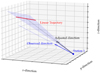Fig. 4 New geometrical perspective based on the coplanarity constraint between each measured direction vector and the trajectory line.

3.1 Functional model and resulting condition equations

As the direction vectors V_i(a_i, b_i, c_i) are introduced as observations subject to random errors, the observation errors $e_{a_{\text{i}}}$, $e_{b_{\text{i}}}$, and $e_{c_{\text{i}}}$ have to be introduced in the functional model, yielding from Eq. (24) the non-linear condition equations $$\begin{array}{l}\left(X_{\text{M}}-X_{\text{S}}\right)\left[b_{\text{M}}\left(c_{\text{i}}-e_{c_{\text{i}}}\right)-c_{\text{M}}\left(b_{\text{i}}-e_{b_{\text{i}}}\right)\right]\hfill \\ -\left(Y_{\text{M}}-Y_{\text{S}}\right)\left[a_{\text{M}}\left(c_{\text{i}}-e_{c_i}\right)-c_{\text{M}}\left(a_{\text{i}}-e_{a_{\text{i}}}\right)\right]\hfill \\ +\left(Z_{\text{M}}-Z_{\text{S}}\right)\left[a_{\text{M}}\left(b_{\text{i}}-e_{b_{\text{i}}}\right)-b_{\text{M}}\left(a_{\text{i}}-e_{a_{\text{i}}}\right)\right]=0,\hfill \end{array}$$(25)

or written equivalently, following the general form of condition equations, as $${\varphi }_i\left(X_{\text{M}},Y_{\text{M}},Z_{\text{M}},a_{\text{M}},b_{\text{M}},c_{\text{M}},e_{a_{\text{i}}},e_{b_{\text{i}}},e_{c_{\text{i}}}\right)=0,$$(26)

with i = 1, …n and n being the number of direction vectors and ϕ_i representing non-linear differentiable functions of the unknown parameters and the errors. This can be expressed in matrix notation as $$\Phi \left(X,e\right)=0,$$(27)

with the formal vector Φ containing the implicit non-linear functional relationship between the error vector $$e={\left[e_{a_1},e_{b_1},e_{c_1},\mathrm{...},e_{a_n},e_{b_n},e_{c_n}\right]}^{\text{T}},$$(28)

which contains the errors of the observations from all stations and the vector of unknown parameters $$X={\left[X_{\text{M}},Y_{\text{M}},Z_{\text{M}},a_{\text{M}},b_{\text{M}},c_{\text{M}}\right]}^{\text{T}}.$$(29)

In this study, we apply the same restrictions for the unknowns as in Borovicka (1990) to obtain a simpler equation system for the following computations. Therefore, setting $X_{\text{M}}=X_{\text{M}}^0$ and a_M = 1, the vector of unknown parameters results in $$X={\left[Y_{\text{M}},Z_{\text{M}},b_{\text{M}},c_{\text{M}}\right]}^{\text{T}}.$$(30)

3.2 Stochastic model taking into account variances and covariances of the observations

In this adjustment problem, the cofactor matrix will have the same structure as in Eq. (15), while for example, the VCM for the first station contains the variances and covariances of the observed directions: $${\Sigma }_{{\text{LL}}_1}=\left|\begin{array}{llllll}{\sigma }_{a_1}^2\hfill & {\sigma }_{a_1{b}_1}\hfill & {\sigma }_a{{}_{{}_1}}_{c_1}\hfill & 0\hfill & \cdots \hfill & 0\hfill \\ {\sigma }_b{{}_{{}_1}}_a{}_{{}_1}\hfill & {\sigma }_{b_1}^2\hfill & {\sigma }_{{\text{b}}_1{c}_1}\hfill & 0\hfill & \cdots \hfill & 0\hfill \\ {\sigma }_c{}_{{}_1{a}_1}\hfill & {\sigma }_{c_1{b}_1}\hfill & {\sigma }_{c_1}^2\hfill & 0\hfill & \cdots \hfill & 0\hfill \\ 0\hfill & 0\hfill & 0\hfill & \ddots \hfill & \hfill & \hfill \\ ⋮\hfill & ⋮\hfill & ⋮\hfill & \hfill & \hfill & \hfill \\ 0\hfill & 0\hfill & 0\hfill & \hfill & \hfill & \hfill \end{array}\right|.$$(31)

For a non-singular dispersion matrix, the respective weight matrix P can be obtained from Eq. (17).

3.3 Stochastic model taking into account the geometry between station and meteor

The presented stochastic model for this adjustment problem can be extended in such a way that the geometry information between each station and the observed meteor is also taken into account. This is allowed, as the weights in the adjustment are relative in the sense that the relationship between the group of observations between each station is of importance. Therefore, an individual variance for the unit weight can be introduced in $$Q_{\text{LL}}=\left|\begin{array}{cccc}\frac{2}{{\sigma }_{0_1}^2}{\Sigma }_{{\text{LL}}_1}& 0& \cdots & 0\\ 0& \frac{1}{{\sigma }_{0_2}^2}{\Sigma }_{{\text{LL}}_2}& \cdots & 0\\ ⋮& ⋮& \ddots & ⋮\\ 0& 0& \cdots & \frac{1}{{\sigma }_{0_m}^2}{\Sigma }_{{\text{LL}}_{\text{m}}}\end{array}\right|.$$(32)

The individual variances of the unit weight can be seen as scaling factors for the observations of each station. Therefore, the computed weights w_i from Eq. (18), expressed by the geometry of each station and the recorded meteor, can be introduced in this stochastic model as a scale factor for each group of observations, yielding $$Q_{\text{LL}}=\left|\begin{array}{cccc}\frac{1}{w_1}{\Sigma }_{{\text{LL}}_1}& 0& \cdots & 0\\ 0& \frac{1}{w_2}{\Sigma }_{{\text{LL}}_2}& \cdots & 0\\ ⋮& ⋮& \ddots & ⋮\\ 0& 0& \cdots & \frac{1}{w_m}{\Sigma }_{{\text{LL}}_{\text{m}}}\end{array}\right|.$$(33)

3.4 Least squares solution within the Gauss-Helmert model

We present a solution for the resulting adjustment problem that is based on the Gauss-Newton approach. This involves a linear approximation of the non-linear condition equations and an approximation of both the unknown parameters and the unknown errors. The studies of Pope (1972), Lenzmann & Lenzmann (2004), and Neitzel & Petrovic (2008) have shown theoretically and numerically that only such a linearisation of the functional model can lead to a rigorous solution within the GH model.

The first-order Taylor series approximation of the formal vector Φ(X, e) at the point X⁰ and e⁰ yields $$\begin{array}{c}\Phi \left(X,e\right)\approx \Phi \left(X^0,e^0\right)+\frac{\partial \Phi \left(X,e\right)}{\partial X}|{}_{X^0\text{,}{e}^0}\left(X-X^0\right)\\ +\frac{\partial \Phi \left(X,e\right)}{\partial e}|{}_{X^0,e^0}\left(e-e^0\right)=0.\end{array}$$(34)

Therefore, we compute as a first step the partial derivatives of the condition equations with respect to the unknown parameters of the problem and form the Jacobian matrix $$A=\frac{\partial \Phi \left(X,e\right)}{\partial X}|{}_{X^0,e^0}=\left[j_{Y_{\text{M}}}\left|j_{Z_{\text{M}}}\right|j_{b_{\text{M}}}|j_{c_{\text{M}}}\right],$$(35)

with the respective vectors $$j_{Y_{\text{M}}}=\left[\begin{array}{c}⋮\\ c_{\text{M}}{}^0\left(a_i-e_{a_i}{}^0\right)-a_{\text{M}}{}^0\left(c_i-e_{c_i}{}^0\right)\\ ⋮\end{array}\right],$$(36) $$j_{Z_{\text{M}}}=\left[\begin{array}{c}⋮\\ a_{\text{M}}{}^0\left(b_i-e_{b_i}{}^0\right)-b_{\text{M}}{}^0\left(a_i-e_{a_i}{}^0\right)\\ ⋮\end{array}\right],$$(37) $$j_{b_{\text{M}}}=\left[\begin{array}{c}⋮\\ \left(X_{\text{M}}{}^0-X_{\text{S}}\right)\left(c_i-e_{c_i}{}^0\right)-\left(Z_{\text{M}}{}^0-Z_{\text{S}}\right)\left(a_i-e_{a_i}{}^0\right)\\ ⋮\end{array}\right]$$(38)

and $$j_{c_{\text{M}}}=\left[\begin{array}{c}⋮\\ \left(Y_{\text{M}}{}^0-Y_{\text{S}}\right)\left(a_i-e_{c_i}{}^0\right)-\left(X_{\text{M}}{}^0-X_{\text{S}}\right)\left(b_i-e_{b_i}{}^0\right)\\ ⋮\end{array}\right].$$(39)

Subsequently, a second Jacobian matrix is formulated that contains the partial derivatives of the condition equations with respect to the unknown errors $$B=\frac{\partial \Phi \left(X,e\right)}{\partial e}|{}_{X^0,e^0}=\left[\begin{array}{llll}{B}_1\hfill & 0\hfill & \cdots \hfill & 0\hfill \\ 0\hfill & B_2\hfill & \cdots \hfill & 0\hfill \\ ⋮\hfill & ⋮\hfill & \ddots \hfill & ⋮\hfill \\ 0\hfill & 0\hfill & \cdots \hfill & B_m\hfill \end{array}\right],$$(40)

with matrices B₁, B₂,…, B_m constructed individually for each station. For example, the respective matrix for the first station can be written as $$B_1=\left[\begin{array}{llllllll}{j}_{e_{a1}}\hfill & j_{e_{b1}}\hfill & j_{e_{c1}}\hfill & 0\hfill & 0\hfill & 0\hfill & 0\hfill & \cdots \hfill \\ 0\hfill & 0\hfill & 0\hfill & j_{e_{a1}}\hfill & j_{e_{b1}}\hfill & j_{e_{c1}}\hfill & 0\hfill & \cdots \hfill \\ 0\hfill & 0\hfill & 0\hfill & 0\hfill & 0\hfill & 0\hfill & \ddots \hfill & \hfill \\ ⋮\hfill & ⋮\hfill & ⋮\hfill & ⋮\hfill & ⋮\hfill & ⋮\hfill & \hfill & \hfill \end{array}\right],$$(41)

with the respective partial derivatives being $$j_{e_a}=b_{\text{M}}{}^0\left(Z_{\text{M}}{}^0-Z_S\right)-c_{\text{M}}{}^0\left(Y_{\text{M}}{}^0-Y_S\right),$$(42) $$j_{e_b}=c_{\text{M}}{}^0\left(X_{\text{M}}{}^0-X_S\right)-a_{\text{M}}{}^0\left(Z_{\text{M}}{}^0-Z_S\right),$$(43)

and $$j_{e_c}=a_{\text{M}}{}^0\left(Y_{\text{M}}{}^0-Y_S\right)-b_{\text{M}}{}^0\left(X_{\text{M}}{}^0-X_S\right).$$(44)

Introducing the Jacobian matrices into Eq. (34) results in the linearised condition equations as $$\Phi \left(X^0,e^0\right)+A\left(X-X^0\right)+B\left(e-e^0\right)=0.$$(45)

Following the usual notation, we introduce the vector of misclosures $$w=\Phi \left(X^0,e^0\right)-B{e}^0,$$(46)

and the vector of reduced unknowns x = X - X⁰ into Eq. (45), resulting in the linearized functional model² $$Ax+Be+w=0.$$(47)

Due to the implicit functional relationship between the unknown parameters of this type of adjustment problem, a least squares solution can be derived by searching for stationary points of the Lagrange function: $$\text{K}\left(x,e,k\right)=e^{\text{T}}Pe-2k^{\text{T}}\left(Be+Ax+w\right),$$(48)

where k denotes the vector of Lagrange multipliers. The iterative procedure for obtaining a least squares solution within the GH model can be found in many textbooks and studies in the geodetic literature, such as those of Niemeier (2008, p. 177) or Malissiovas (2019, p. 40 ff.). In the following we present this procedure for solving the discussed problem.

The system of normal equations can be derived by $$\begin{array}{r}\hfill \frac{\partial \text{K}}{\partial e^{\text{T}}}=2P\tilde{e}-2B^{\text{T}}\widehat{k}=0\\ \hfill \Rightarrow \tilde{e}=Q_{\text{LL}}{B}^{\text{T}}\widehat{k},\end{array}$$(49) $$\begin{array}{r}\hfill \frac{\partial \text{K}}{\partial x^{\text{T}}}=-2{\widehat{k}}^{\text{T}}A=0\\ \hfill \Rightarrow A^{\text{T}}\widehat{k}=0,\end{array}$$(50) $$\frac{\partial \text{K}}{\partial K^{\text{T}}}=-2\left(B\tilde{e}+A\widehat{x}+w\right)=0.$$(51)

The tilde symbol denotes a prediction, while the circumflex an estimator. Introducing the error vector from Eqs. (49) into (51) yields the reduced normal equations $$B{Q}_{\text{LL}}{B}^{\text{T}}\widehat{K}+A\widehat{x}\text{+}w=0.$$(52)

Furthermore, Eqs. (50) and (52) can be expressed in block matrix form as $$\left[\begin{array}{cc}B{Q}_{\text{LL}}{B}^{\text{T}}& A\\ A^{\text{T}}& 0\end{array}\right]\left[\begin{array}{c}\widehat{k}\\ \widehat{x}\end{array}\right]=\left[\begin{array}{c}-w\\ 0\end{array}\right],$$(53)

that leads to the solution of $$\left[\begin{array}{c}\widehat{k}\\ \widehat{x}\end{array}\right]={\left[\begin{array}{cc}B{Q}_{\text{LL}}{B}^{\text{T}}& A\\ A^{\text{T}}& 0\end{array}\right]}^{-1}\left[\begin{array}{c}-w\\ 0\end{array}\right].$$(54)

For a non-singular product [BQ_LLB^T] it is possible to explicitly express an estimate for the vector of reduced unknowns $$\widehat{x}\text{=}{N}^{-1}n\text{,}$$(55)

and the vector of Lagrange multipliers $$\widehat{k}=-{\left(B{Q}_{\text{LL}}{B}^{\text{T}}\right)}^{-1}\left(A\widehat{x}+w\right),$$(56)

after introducing the normal matrix $$N=-\left[A^{\text{T}}{\left(B{Q}_{\text{LL}}{B}^{\text{T}}\right)}^{-1}A\right]$$(57)

and the vector $$n=A^{\text{T}}{\left(B{Q}_{\text{LL}}{B}^{\text{T}}\right)}^{-1}w.$$(58)

Finally, an estimate for the vector of unknown parameters can be derived by $${\widehat{X}}_i={\widehat{x}}_i+X^0,$$(59)

and a prediction for the errors from Eq. (49). A series of linearised adjustments within the GH model have to be computed because of the iterative nature of the Gauss-Newton approach. Therefore, the estimated vector $\widehat{X}$ is used as the vector of initial values for the subsequent iteration step: $$X_{i+1}^0={\widehat{X}}_i,$$

and the predicted error, excluding for a moment its random character, as $$e_{i+1}^0={\tilde{e}}_i.$$(60)

The vector of adjusted observations can be finally computed as $$\widehat{L}=L-{\tilde{e}}_{\text{final}},$$(61)

with the subscript ‘final’ denoting the last iteration step of the procedure.

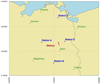Fig. 5 Map illustrating the geometry between the stations and the projection of the synthetic meteor (ground track) depicted with the red arrow.

Error estimation

The error estimates of the adjustment results can be easily computed in terms of the cofactor matrices of the unknown parameters $Q_{\widehat{\text{X}}\widehat{\text{X}}}$ of the errors $Q_{\tilde{\text{e}}\tilde{\text{e}}}$ and the adjusted observations $Q_{\widehat{\text{L}}\widehat{\text{L}}}$. These cofactor matrices can be obtained using standard procedures, presented for example in Niemeier (2008, p. 178) or Malissiovas (2019, p. 44 ff.).

4 Numerical example

A set of synthetic observations were generated using the simulation tool implemented for the study of meteor showers (Margonis et al. 2018). These observations were used as an input to the different methods described in this work. The intention of our synthetic setup is to reveal the limitations of a trajectory solution when geometric aspects alone are taken into account.

Our hypothetical scenario consists of four observing stations which simultaneously register a meteor. Two of the stations (A, D) have a favourable geometry but the measurements are of relatively low precision (e.g. use of low-resolution cameras). The other two stations (B, C) have a less favourable geometry, as they are located close to the projection of the trajectory line. However, these measurements are more precise compared to the ones made from A and D (e.g. use of high-resolution cameras; Fig. 5). Three observation vectors from each station were used: at the beginning, at the middle, and at the end of the meteor trail. The trajectory solution consists of a point on the meteor trail and the moving direction.

For the simulated meteor event, the following entry parameters were assigned:

• (i)

  geodetic coordinates of the meteor position at t₀ = 0;

• (ii)

  duration of the meteor ∆t in seconds;

• (iii)

  speed of the meteor in km s⁻¹;

• (iv)

  horizontal coordinates of the trail orientation with respect to the local plane of a station;

• (v)

  geodetic coordinates of the observing stations.

The geodetic coordinates at the beginning and end point of the meteor along with those of each station are given in Table 1. The moving orientation of the meteor was defined with reference to the local coordinate system of station A. The azimuth of the moving direction was Az = 10° measuring from north to west while the elevation angle, which corresponds to the entrance angle of the meteor, was El = 25°. The speed of the meteor was assumed to be v = 19 kms−¹. From the known orientation and moving speed of the meteor, the velocity vector can be calculated.

For our computations, all direction (unit) vectors were trans-formed to the Earth-centred Earth-fixed (ECEF) coordinate system, with $$\begin{array}{l}X=\cos \text{\hspace{0.17em}Az\hspace{0.17em}sin\hspace{0.17em}E1,}\hfill \\ Y=\sin \text{\hspace{0.17em}Az\hspace{0.17em}sin\hspace{0.17em}E1,}\hfill \\ Z=\cos \text{\hspace{0.17em}E}1.\hfill \end{array}$$(62)

The direction vectors from each station (a_i, b_i, c_i) to the meteor at time intervals t₀, t_∆t/2, and t_∆t were calculated by simply sub-tracting the position vectors of the meteor P_M (X_M, Y_M, Z_M) from the position vectors of the station P_S (X_S, Y_S, Z_S).

In our example, we assume that the observations between the four stations have different standard deviations. The difference in the quality of the measurements, when derived from optical systems, may result for example from the use of sensors of different quality or from following different calibration procedures. Given in spherical coordinates at first, the direction vectors from sta-tions A and D were taken with a standard deviation of σ_{A D} = 1° in both azimuth and elevation, whereas from stations B and C, σ_b,c = 0.1°. Assuming uncorrelated spherical coordinates for simplicity, we can form a diagonal variance–covariance matrix Σ_AzEl

As all computations in this article were made in a rectangular coordinate system, the initial stochastic information has to be converted to the same coordinate system by applying the law of error propagation. Therefore, the cofactor matrix of the direction vectors in rectangular coordinates can be computed using the rules of error propagation, resulting in $${\Sigma }_{\text{abc}}=F{\Sigma }_{\text{AZE1}}{F}^{\text{T}}.$$(63)

Matrix F contains the partial derivatives of the non-linear relationships in Eq. (62) with respect to the spherical coordinates. The derived VCM Σ_abc used to compute the cofactor matrix Q_llor the adjustment in the GH model from Eq. (15).

In the next step, the calculated variances were used to generate normally distributed random errors for each station individually, which were added respectively to the LoS measurements. For the interested reader, the values of the observed direction vectors, their standard deviations, and the geometrical weights for each station are listed in Tables A.3 and A.5 of the Appendix, respectively. Consequently, two least squares solutions were computed for the simulated data. First, by applying the SLLS method described in Sect. 2.3 and the newly presented solution within the GH model from Sect. 3.4. For completeness, the solution of the GH with the extended stochastic model is also presented. The values of the estimated parameters and their standard deviations are shown in Table 2.

The initial values for the unknown parameters X given in Eq. (29) are calculated using the plane-plane intersection method between the first two stations A and B. For our numerical example, the approximated values X° = $\left[X_{\text{M}}^0,Y_{\text{M}}^0,Z_{\text{M}}^0,a_{\text{M}}^0,b_{\text{M}}^0,c_{\text{M}}^0\right]$ were equal to $X_{\text{M}}^0=3794.49124$, $Y_{\text{M}}^0=898.85936$, $Z_{\text{M}}^0=5095.39098$ for the point on the estimated trajectory line, while the vector components were $a_{\text{M}}^0=0.87506$, $b_{\text{M}}^0=0.29339$, $c_{\text{M}}^0=-0.38496$.

An interesting finding is the amount of discrepancy in the direction of the trajectory line, which can be interpreted as an angular displacement D_rad of the radiant, that is the point in the sky where the meteor appears to originate. This will be equal to D_rad = 3.55°, D_rad = 0.88°, and D_rad = 0.25° for the SLLS method, the GH model and the GH with the extended stochastic model respectively.

The solutions presented in Table 2 and the angular distances between the simulated and the estimated trajectory lines suggest, as anticipated, a difference in the results of the two methods. The solution obtained by the SLLS method is influenced by the observations acquired by the low-resolution camera systems in stations A and D to a greater degree. These two stations have a better viewing geometry compared to stations B and C which results in a higher weight in the adjustment. The extended stochastic model offers a hybrid solution, in that the accuracy of the measurements and the geometrical configuration between the stations and the meteor influence the estimated trajectory.

The use of different stochastic models for the observations leads to different standard deviations for the adjusted unknowns. Beyond the aim for the lowest possible numerical values for the standard deviations, there is of course the demand for values that are as realistic as possible. Under this premise, the solution GH with an extended stochastic model appears to be the most appropriate, as both the measurement accuracy and the measurement configuration are taken into account in the stochastic model.

The effect of each adjustment approach to the estimated trajectory line is comprehensively shown in Fig. 6. This is a graphical representation of the orthogonal distances D between the measured direction vectors and each estimated trajectory line, computed by Eq. (11) for all adjustment solutions. As expected, each set of observed direction vectors for a given station contributes differently to the estimation of the trajectory in the GH approach. The juxtaposition of the low resolution measurements of stations A and D, and the high resolution of stations B and C is clearly projected to the computed orthogonal distances, depicted in orange and blue, respectively, in Fig. 6. It can be seen that low-resolution measurements lead to smaller weights in the adjustment and higher values for the orthogonal distances, as these measurements would contribute less to the solution of the trajectory line.

The solution GH with an extended stochastic model can be regarded as a reference solution, as both the measurement accuracy and the measurement configuration are taken into account in the stochastic model. The extent to which the other solutions, namely GH and SLLS, differ from this reference solution depends on the number of observations and stations as well as on the measurement configuration and can therefore not be given in a generalised form. However, depending on the type and extent of information on the accuracies and configuration of the measurements, the user is now able to properly take this information into account in the stochastic model when computing the trajectory line of a meteor.

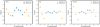Fig. 6 Values of the orthogonal distances calculated for each approach following Eq. (11). From left to right: computed values for the SLLS method, the GH, and the GH with the extended stochastic model are shown, respectively. Highlighted symbols in orange indicate calculated values derived from low-resolution observations, i.e. measurements obtained from stations A and D. The straight dashed line represents the estimated trajectory line for each approach.

5 Conclusion

This study sets out with the aim of assessing the importance of including more realistic stochastic information for the direction vectors when estimating the linear flight path of a mete-oroid. Detailed explanations of the two most popular approaches in the literature, namely the plane-intersection method of Ceplecha (1987) and the SLLS approach of Borovicka (1990), are presented in Sect. 2 accompanied by the corresponding mathematical formulations. It is noted that especially the latter approach postulates a geometry-based stochastic model, disregarding any existing a priori stochastic information about the observed direction vectors.

A novel geometric perspective for the discussed adjustment problem is presented in Sect. 3, based on the coplanarity condition between each adjusted direction vector and the linear meteor trajectory. An iterative least squares solution within the GH model has been described in detail, which is based on the Gauss-Newton approach and allows the consideration of the a priori stochastic information of the observed direction vectors directly in the stochastic model. Additionally, an extended stochastic model is presented that allows the integration of the geometry information between the observed group of directions from each station.

The results of this study show a discrepancy between the SLLS method and the GH approach described in this work. Although a single numerical example is presented here, we anticipate that the computation of the trajectory line for various geometrical configurations between a meteoroid and the observing stations will yield different results when implementing the methods presented in this study. It is therefore possible that the use of the stochastic information leads to a more realistic solution for the trajectory line of a meteoroid.

A combined solution which takes into account the full 3D motion of the meteoroid including velocity and deceleration parameters and incorporates their uncertainties directly in the adjustment has yet to be investigated. Other effects that may divert the flight path of a meteoroid from a straight line, such as the rotation of the Earth or the influence of the Earth’s gravity field, need to be considered when calculating the true radiant of a meteor. Furthermore, physical processes during the atmospheric entry of a meteoroid, such as fragmentation or aerodynamic effects, may increase the complexity of a trajectory solution.

Acknowledgements

The authors of this study would like to gratefully acknowledge Dr. Jiři Borovička for his valuable comments and suggestions for the improvement of this paper. This work was funded in part by the Deutsch Forschungsgemeinschaft (DFG – German Research Foundation) under the grant number OB 124/20-1.

Appendix A LoS measurements and stochastic models

In this Appendix we provide all necessary data for the computations of the numerical example. Interested readers who need further information are welcome to contact the authors directly. The rectangular coordinates of the meteor and the stations are given in Table A.1 and Table A.2 respectively. Table A.3 lists the synthetic direction vectors, which are utilized as observations in the adjustment for the estimation of the meteor line. Table A.4 lists the submatrices for the VCM of each station computed from (63). For example, for the first station this will be $${\Sigma }_{{\text{LL}}_1}=\left[\begin{array}{lll}{\Sigma }_{{\text{LL}}_{\text{A1}}}\hfill & 0\hfill & 0\hfill \\ 0\hfill & {\Sigma }_{{\text{LL}}_{\text{A}2}}\hfill & 0\hfill \\ 0\hfill & 0\hfill & {\Sigma }_{{\text{LL}}_{\text{A3}}}\hfill \end{array}\right].$$

Additionally, taking into account the geometrical weights computed from (18) and listed in Table A.5, it is possible to set up the cofactor matrix of Eq. (33).

References

All Tables

All Figures

	Fig. 1 Schematic illustration of the observation of a linear trajectory from two locations.
In the text

	Fig. 2 Geometric representation of the solution estimated by the plane intersection method from two stations.
In the text

	Fig. 3 Simplified geometric representation of the SLLS method.
In the text

	Fig. 4 New geometrical perspective based on the coplanarity constraint between each measured direction vector and the trajectory line.
In the text

	Fig. 5 Map illustrating the geometry between the stations and the projection of the synthetic meteor (ground track) depicted with the red arrow.
In the text

Fig. 6 Values of the orthogonal distances calculated for each approach following Eq. (11). From left to right: computed values for the SLLS method, the GH, and the GH with the extended stochastic model are shown, respectively. Highlighted symbols in orange indicate calculated values derived from low-resolution observations, i.e. measurements obtained from stations A and D. The straight dashed line represents the estimated trajectory line for each approach.

In the text

References

- Borovicka, J. 1990, Bull. Astron. Inst. Czechoslovakia, 41, 391 [NASA ADS] [Google Scholar]
- Bronshtein, I., Semendyayev, K., Musiol, G., & Muehlig, H. 2007, Handbook of Mathematics, 5th edn. (Berlin Heidelberg New York: Springer) [Google Scholar]
- Ceplecha, Z. 1987, Bull. Astron. Inst. Czechoslovakia, 38, 222 [NASA ADS] [Google Scholar]
- Colas, F., Zanda, B., Vernazza, P., et al. 2012, in Asteroids, Comets, Meteors (New York: HarperCollins), 1667, 6426 [NASA ADS] [Google Scholar]
- Egal, A., Gural, P.S., Vaubaillon, J., Colas, F., & Thuillot, W. 2017, Icarus, 294, 43 [NASA ADS] [CrossRef] [Google Scholar]
- Ghilani, C.D. 2018, Adjustment Computations: Spatial Data Analysis, 6th edn. (Hoboken, NJ, USA: John Wiley and Sons) [Google Scholar]
- Gural, P.S. 2012, Meteor. Planet. Sci., 47, 1405 [NASA ADS] [CrossRef] [Google Scholar]
- Howie, R.M., Paxman, J., Bland, P.A., et al. 2017, Meteor. Planet. Sci., 52, 1669 [NASA ADS] [CrossRef] [Google Scholar]
- Jeanne, S., Colas, F., Zanda, B., et al. 2019, A&A, 627, A78 [EDP Sciences] [Google Scholar]
- Jenniskens, P., Gural, P.S., Dynneson, L., et al. 2011, Icarus, 216, 40 [NASA ADS] [CrossRef] [Google Scholar]
- Lenzmann, L., & Lenzmann, E. 2004, Allgemeine Vermessungs-Nachr., 111, 68 [Google Scholar]
- Malissiovas, G. 2019, New Nonlinear Adjustment Approaches for Applications in Geodesy and Related Fields (Munchen: Ausschuss Geodasie der Bayerischen Akademie der Wissenschaften (DGK)), C, 841 [Google Scholar]
- Malissiovas, G., Neitzel, F., & Petrovic, S. 2016, J. Geodetic Sci., 6, 43 [NASA ADS] [CrossRef] [Google Scholar]
- Margonis, A., Christou, A., & Oberst, J. 2018, A&A, 618, A99 [NASA ADS] [CrossRef] [EDP Sciences] [Google Scholar]
- Neitzel, F., & Petrovic, S. 2008, Zeitschrift fur Geodasie, Geoinformation und Landmanagement, 133, 141 [Google Scholar]
- Niemeier, W. 2008, Ausgleichungsrechnung, (in German) 2nd edn. [Adjustment computations] (New York: Walter de Gruyter) [CrossRef] [Google Scholar]
- Perovic, G. 2005, Least Squares (Monograph) (Faculty of Civil Engineering, University of Belgrade) [Google Scholar]
- Pope, A. 1972, In: Proceedings of the 38th Annual Meeting of the American Society of Photogrammetry, Washington, DC, 449 [Google Scholar]
- Sansom, E.K., Rutten, M.G., & Bland, P.A. 2017, AJ, 153, 87 [NASA ADS] [CrossRef] [Google Scholar]
- Sansom, E.K., Jansen-Sturgeon, T., Rutten, M.G., et al. 2019, Icarus, 321, 388 [NASA ADS] [CrossRef] [Google Scholar]
- Vida, D., Gural, P.S., Brown, P.G., Campbell-Brown, M., & Wiegert, P. 2020, MNRAS, 492, 5313 [NASA ADS] [CrossRef] [Google Scholar]
- Wolf, H. 1978, Zeitschrift fur Vermessungswesen, 103, 41 [Google Scholar]
The restriction of Eq. (7) prevents the computation of planes that are parallel to the z-axis.
Similar to the definitions from Wolf (1978) or Perovic (2005, p. 203), the developed linearised functional model Eq. (47) accompanied by the stochastic model Eq. (15) results in the well-known GH model.
All Tables
Estimated values for the unknown parameters and their standard deviations calculated from the SLLS method, the GH, and the GH with the extended stochastic model, being compared with the simulated values.