| Issue |
A&A
Volume 662, June 2022
|
|
|---|---|---|
| Article Number | A60 | |
| Number of page(s) | 13 | |
| Section | Extragalactic astronomy | |
| DOI | https://doi.org/10.1051/0004-6361/202142871 | |
| Published online | 16 June 2022 | |
Molecular gas in z ∼ 6 quasar host galaxies
1
INAF – Osservatorio di Astrofisica e Scienza dello Spazio di Bologna, via Gobetti 93/3, 40129 Bologna, Italy
e-mail: This email address is being protected from spambots. You need JavaScript enabled to view it.
2
Dipartimento di Fisica e Astronomia, Alma Mater Studiorum, Universitá di Bologna, Via Gobetti 93/2, 40129 Bologna, Italy
3
Dipartimento di Fisica “G. Occhialini”, Università degli Studi di Milano-Bicocca, Piazza della Scienza 3, 20126 Milano, Italy
4
Max-Planck Institut für Astronomie, Königstuhl 17, 69117 Heidelberg, Germany
5
Leiden Observatory, Leiden University, PO Box 9513 2300 RA Leiden, The Netherlands
6
National Radio Astronomy Observatory, Pete V. Domenici Array Science Center, PO Box O Socorro, NM 87801, USA
7
Argelander-Institute for Astronomy, University of Bonn, Auf dem Hügel 71, 53121 Bonn, Germany
8
Sorbonne Université, UPMC Université Paris 6 & CNRS, UMR 7095, Paris, France
9
Institut d’Astrophysique de Paris, 98b boulevard Arago, 75014 Paris, France
10
Steward Observatory, University of Arizona, 933 N. Cherry St., Tucson, AZ 85721, USA
11
Gemini Observatory, NSF’s NOIRLab, 670 N A’ohoku Place, Hilo, Hawai’i 96720, USA
12
Department of Physics, Winona State University, Winona, MN 55987, USA
13
ICRAR M468, The University of Western Australia, 35 Stirling Hwy, Crawley, WA 6009, Australia
14
Research School of Astronomy and Astrophysics (RSAA), Australian National University, ACT 2611, Australia
15
Department of Astronomy, School of Physics, Peking University, 5 Yiheyuan Road, Haidian District, Beijing 10087, PR China
16
Kavli Institute of Astronomy and Astrophysics at Peking University, 5 Yiheyuan Road, Haidian District, Beijing 100871, PR China
17
Department of Astronomy, Tsinghua University, Beijing 100084, PR China
18
European Southern Observatory, Alonso de Córdova 3107, Vitacura, Región Metropolitana, Chile
19
Institut de Radioastronomie Millimétrique (IRAM), 300 Rue de la Piscine, 38400 Saint-Martin-d’Hères, France
20
Department of Astronomy, Cornell University, Space Sciences Building, Ithaca, NY 14853, USA
21
Astronomy Department, California Institute of Technology, MC249-17, Pasadena, California 91125, USA
22
Max-Planck-Institut für Radioastronomie, Auf dem Hügel 69, 53121 Bonn, Germany
Received:
9
December
2021
Accepted:
6
March
2022
Abstract
We investigate the molecular gas content of z ∼ 6 quasar host galaxies using the Institut de Radioastronomie Millimétrique Northern Extended Millimeter Array. We targeted the 3 mm dust continuum, and the line emission from CO(6–5), CO(7–6), and [C I]2−1 in ten infrared–luminous quasars that have been previously studied in their 1 mm dust continuum and [C II] line emission. We detected CO(7–6) at various degrees of significance in all the targeted sources, thus doubling the number of such detections in z ∼ 6 quasars. The 3 mm to 1 mm flux density ratios are consistent with a modified black body spectrum with a dust temperature Tdust ∼ 47 K and an optical depth τν = 0.2 at the [C II] frequency. Our study provides us with four independent ways to estimate the molecular gas mass, MH2, in the targeted quasars. This allows us to set constraints on various parameters used in the derivation of molecular gas mass estimates, such as the mass per luminosity ratios αCO and α[CII], the gas-to-dust mass ratio δg/d, and the carbon abundance [C]/H2. Leveraging either on the dust, CO, [C I], or [C II] emission yields mass estimates of the entire sample in the range MH2 ∼ 1010–1011 M⊙. We compared the observed luminosities of dust, [C II], [C I], and CO(7–6) with predictions from photo-dissociation and X-ray dominated regions. We find that the former provide better model fits to our data, assuming that the bulk of the emission arises from dense (nH > 104 cm−3) clouds with a column density NH ∼ 1023 cm−2, exposed to a radiation field with an intensity of G0 ∼ 103 (in Habing units). Our analysis reiterates the presence of massive reservoirs of molecular gas fueling star formation and nuclear accretion in z ∼ 6 quasar host galaxies. It also highlights the power of combined 3 mm and 1 mm observations for quantitative studies of the dense gas content in massive galaxies at cosmic dawn.
Key words: galaxies: high-redshift / galaxies: evolution / galaxies: ISM / galaxies: star formation / quasars: emission lines
© ESO 2022
1. Introduction
Quasars residing in the so-called cosmic dawn (z ≳ 6, age of the Universe < 1 Gyr) were first discovered at the turn of the century (e.g., Fan et al. 2000, 2003). To date, we know ∼400 quasars at z > 5.5, including three at z > 7.5 (Bañados et al. 2018; Yang et al. 2020; Wang et al. 2021). Multiwavelength campaigns, in particular at submillimeter and millimeter (hereafter, mm) wavelengths, revealed that these early quasars reside in extremely active galaxies, experiencing intense starbursts (with star formation rates SFR = 100–1000 M⊙ yr−1; Bertoldi et al. 2003; Wang et al. 2008a,b; Drouart et al. 2014; Leipski et al. 2014; Venemans et al. 2018) and fast, radiatively efficient black hole accretion (ṀBH > 10 M⊙ yr−1; De Rosa et al. 2014; Schindler et al. 2020; Yang et al. 2021). This rapid gas consumption depletes the immense reservoirs of molecular gas (MH2 > 1010 M⊙; Walter et al. 2003; Wang et al. 2010; Venemans et al. 2017a; Decarli et al. 2018) of the host galaxies, which can be refueled via accretion of cool gas from the circumgalactic medium (e.g., Farina et al. 2019; Drake et al. 2019) or via mergers with gas–rich galaxies (e.g., Trakhtenbrot et al. 2017; Decarli et al. 2017, 2019; Vito et al. 2019).
Both star formation and black hole accretion release huge amounts of energy which could affect the evolution of the host galaxies: Mechanical feedback (via winds or jets) can displace and even remove the gas reservoir; and radiative feedback can heat-up and excite the interstellar medium (ISM) thus slowing down or preventing cooling and gas fragmentation (see Fabian 2012; Heckman & Best 2014; King & Pounds 2015; Somerville & Davé 2015, for reviews on this topic). A quantitative description of the cold (T < 100 K) ISM, poised to constrain the mass, density, temperature, and excitation mechanism of the molecular gas in the quasar hosts, would shed light on the interplay between the ISM, star formation and nuclear activity.
In distant galaxies, the molecular gas mass, MH2, is usually inferred based on photometry covering the Rayleigh-Jeans part of the dust continuum emission (see, e.g., Groves et al. 2015; Scoville et al. 2017a), or via far-infrared emission lines of species such as the carbon monoxide, 12C16O (hereafter, CO; see, e.g., Walter et al. 2003; Wang et al. 2011, as well as the review in Carilli & Walter 2013), neutral carbon (in particular the fine-structure transitions [C I]1−0 and [C I]2−1; see, e.g., Popping et al. 2017; Valentino et al. 2018; Boogaard et al. 2020), or singly ionized carbon (via the bright [C II]3/2−1/2 line; see Venemans et al. 2017b; Zanella et al. 2018). All of these methods rely on a set of assumptions and conversion factors: for example, the gas-to-dust ratio, δg/d (see, e.g., Berta et al. 2016) or the αCO factor that links the luminosity of the CO(1−0) ground transition with the associated molecular gas mass (see Bolatto et al. 2013, for a review). These factors carry implicit dependencies on the metallicity and other properties of the galaxy. Comparisons of MH2 estimates obtained via different prescriptions are pivotal to pin down systematics in the mass determinations. For instance, Dunne et al. (2021) used a combination of dust continuum, CO(1–0) and [C I]1−0 line emission to gauge the molecular gas mass in a sample of massive galaxies at z = 0.35. Because four unknown quantities (molecular gas mass, carbon abundance, αCO, δg/d) are constrained with three observables, only relative values can be directly measured; however, by using additional information (e.g., from their sample variance), mean values for the calibration factors can be inferred. Similarly, Sommovigo et al. (2021, 2022) proposed to use a combination of nested scaling relations to constrain the dust temperature, Td, from the [C II] line luminosity.
The combination of different diagnostics of the cold ISM also reveal some precious information on the physical conditions of the gas. For instance, models of Photo-Dissociation Regions (PDRs) or X-ray Dominated Regions (XDRs) account for various chemical and radiative processes that take place in a gas cloud that is illuminated by an external radiation field in order to predict the emerging intensity of various lines. The former set of models assume that the excitation is driven by the UV radiation from young stars, and they are thus best suited to describe the emission of molecular clouds invested by the radiative output of an on-going starburst. The latter models assume the presence of a strong X-ray radiation field as the driver of the cold gas heating and excitation. These models are hence best suited to account for the quasar contribution to the excitation budget, although both PDR and XDR models have been extensively used in a wide range of astrophysical applications (e.g., Tielens & Hollenbach 1985; Maloney et al. 1996; Meijerink et al. 2007; Goicoechea et al. 2019; Vallini et al. 2019). By exploiting differences in the predicted line emission in PDRs versus XDRs, we can infer hints on the role of different radiative mechanisms (star formation or nuclear activity) that may drive the excitation of the cold ISM. Dust, [C II], [C I], and CO(7–6) form an observationally convenient suite of diagnostics, as with only two frequency settings (one covering the [C II], and one covering [C I] and CO(7–6), together with their respective underlying continuum) we can secure a rich collection of tracers of the cold interstellar medium.
In this study, we present the first systematic campaign targeting CO(7–6) and [C I] in a sample of ten z ∼ 6 quasars. In addition, the unprecedented bandwidth capabilities of new mm receivers together with upgraded correlators enable to observe CO(6–5) as well in the same frequency setting as CO(7–6) and [C I], for certain redshift windows. We used the Plateau de Bure Interferometer (PdBI), later upgraded to the NOrthern Extended Millimeter Array (NOEMA) of the Institut de Radioastronomie Millimétrique (IRAM) to secure CO(6–5), CO(7–6) and [C I] coverage in the 3mm atmospheric window. All of these quasars have been previously detected in the [C II] and dust continuum emission. The paper is structured as follows: in Sect. 2, we introduce the sample, the observations, and the data reduction. In Sect. 3, we present our results, our estimates of MH2 based on various methods, and our constraints on the physical properties of the ISM. We draw our conclusions in Sect. 4. Throughout this paper we assume a ΛCDM cosmology, with H0 = 70 km s−1 Mpc−1, Ωm = 0.3, and ΩΛ = 0.7, and a Kroupa initial mass function to compute star formation rates (SFR)1. In this cosmological framework, the scale distance at z = 6.00 is 5.713 kpc arcsec−1, the luminosity distance is DL = 57.742 Gpc, and the age of the Universe is 914 Myr. The notation ν refers to rest–frame frequencies.
2. Observations and data processing
2.1. Sample
Our goal is to capitalize on the combination of [C II], [C I], CO, and the underlying dust continuum emission to study the molecular medium in quasar host galaxies at the dawn of cosmic time. To this purpose, we selected all of the quasars with previously published [C II] detections. At the time of designing the main part of this program (March 2019), out of ∼150 quasars known at z ≳ 6, fourty-six were detected in [C II]. From these, only nine had previously been observed in their CO(7–6) emission: one (PSO J183.1124+05.0926) is currently unpublished (Decarli et al. in prep.), and two show no line detection (ULAS J1120+0641, ULAS J1342+0928; see Venemans et al. 2017b and Novak et al. 2019). The remaining six quasars (SDSS J1148+5251, VIK J0109–3047, VIK J0305–3150, VIK J2348–3054, SDSS J0100+2802, UHS J0439+1634) have CO(7–6) observations published in Riechers et al. (2009), Venemans et al. (2017a), Wang et al. (2019), and Yang et al. (2019). We removed all of the sources previously observed in CO(7–6) from our selection. We also removed 12 additional quasars that reside at 5.9 ≲ z ≲ 6.1, as at these redshifts the CO(7–6) + [C I] lines are significantly affected by poorer atmospheric transmission. We also removed six quasars that have IR luminosity LIR < 1012 L⊙, that is, quasars are likely too faint at IR wavelengths for our survey. Finally, we drop 11 quasars that lie at declination < − 10° for the sake of observability from NOEMA. In addition to this sample, we include previously unpublished observations of the quasars SDSS J0338+0021 (z = 5.0267) and SDSS J2054-0005 (z = 6.0391). The resulting list of targets thus consists of ten quasars (see Table 1).
Sample of quasars studied in this work.
2.2. Observations and data reduction
The dataset consists of the collection of a main survey and a number of smaller programs conducted at NOEMA and previously at PdBI, for a total observing time of ∼70 h on source (eight antennas equivalent). The half power beam width of NOEMA’s 15 m antennas is ≈48.6″ at 100 GHz. Observations were mostly carried out under average or poor weather conditions with precipitable water vapor columns typically ≳5 mm and system temperatures of 80–200 K with the array in compact (C or D) configuration. We processed the data using clic from the GILDAS2 suite. Table 2 provides a summary of our observations.
Summary of the observations presented in this paper.
J0338+0021 was observed on August 1, and September 28, 2008 (program ID: S052), using the narrow-band 2 mm receiver, and again in July 2013 (program ID: X04D) using WideX. The sources 3C454.3 and MWC349 were observed for bandpass and flux calibration. We observed J0406+066 as amplitude and phase calibrator. The final cube includes 7200 visibilities, corresponding to 9.0 h (five-antenna equivalent).
J2054–0005 was observed in October–November 2013 (program ID: X04D). We used the WideX correlator and tuned the receiver to secure the [C I] and CO(7–6) lines in a single setup. The sources 3C454.3 and MWC349 were observed for bandpass and flux calibration. For the amplitude and phase calibration, we observed 2059+034. The final cube includes 16881 visibilities, corresponding to 21.10 h (five-antenna equivalent).
PJ036+03 was observed in multiple short tracks in June–July 2015 (program ID: S15DA) and June–July 2017 (program ID: S17CD), in compact array configuration (5D and 6D in 2015; 7D and 8D in 2017) using the WideX correlator. The receiver was tuned to encompass the two CO(6–5) and CO(7–6) lines in two independent frequency settings. The calibration sources include the blazar 3C454.3 for bandpass calibration, the source MWC349 for absolute flux calibration, and the quasar 0215+015 for amplitude and phase calibration. The final cubes consist of a total of 22440 visibilities (13.33 h on source, assuming seven antennas) on the CO(7–6) line, and 22317 visibilities (13.28 h on source, assuming seven antennas) on CO(6–5).
The quasar PJ338+29 was observed in July 2018 (program ID: S18DM). The expanded bandwidth offered by the PolyFix correlator enables to encompass the CO(6–5) and CO(7–6) lines in our targets using a single frequency setting. The blazar 3C454.3 served as bandpass calibrator, MWC349 as absolute flux calibrator, and the quasars 2234+282 and J2217+243 as amplitude and phase calibrators. The final cubes comprises a total of 8670 visibilities (3.87 h on source, eight-antenna equivalent).
We observed the quasar J2219+0102 as part of two programs, one covering the CO(5-4) and CO(6–5) lines (August–September 2018, program ID: S18DM), and one covering the CO(6–5), CO(7–6) and [C I] lines (June 2019, program ID: S19DM). The bright sources 3C454.3 and MWC349 acted as bandpass and flux calibrators, while the quasars 2216-038 and 2223-052 were observed as amplitude and phase calibrators. We reduced the two settings independently, and then merged the visibilities in the overlapping frequency range. The 2018 and 2019 observations comprise 13380 and 8640 visibilities, respectively, corresponding to 5.97 and 3.86 h on source (eight-antenna equivalent).
We observed the remaining targets between June 2019 and January 2020 (program ID: S19DM). The observations of PJ159-02 relied on 0851+202, LKHA101, and J1028-0236 as bandpass, flux, and phase and amplitude calibrators respectively. The final cube consists of 7170 visibilities (2.0 h on source, ten-antenna equivalent). Observations of J1319+0950 were performed in excellent weather conditions (precipitable water vapor < 2 mm, system temperature Tsys = 55–70 K) and used on the calibrators 3C273 (bandpass), MWC349 (flux), and 1307+121 (phase, amplitude, pointing, focus). The final cubes consists of 8310 visibilities (2.88 h on source, nine-antenna equivalent). Observations of the quasar J1048-0109 were performed using 3C84, 3C273, and LKHA101 as bandpass and flux calibrators, and 1055+018 as phase and amplitude calibrator. The final cube consists of 10170 visibilities (3.53 h on source, nine-antenna equivalent). We calibrated the observations of the quasar J1104+2134 using MWC349, 0851+202, 3C273, 0923+392 for flux and bandpass calibration; and 1040+244 for phase and amplitude. The final cube consists of 12660 visibilities (4.40 h on source, nine-antenna equivalent). Finally, the observations of PJ359-06 capitalized on 3C454.3, MWC349, and 0003-066 for bandpass, flux, and amplitude and phase calibration. The final cube comprises 3.46 h on source (nine-antenna equivalent).
2.3. Imaging
We imaged the cubes using the GILDAS suite mapping. Natural weighting was adopted in all the cases. The beam FWHM ranges between 3″ and 7″ (see Table 2). We resampled the spectral axis in 50 km s−1 wide channels (computed at the CO(7–6) frequency). In creating the continuum images, we first masked out the channels where strong emission lines are found, based on visual inspection of the spectra. When no obvious lines were detected, we masked out a range of ∼600 km s−1 around the expected frequency of the lines. We created continuum images from the lower and upper side bands independently using the unmasked channels, and use them to subtract from the cubes using the task uv_subtract. Finally, we created continuum–subtracted line maps using the channels within the line full width at zero intensity. In the absence of an obvious line detection, we used a 6 channels (300 km s−1) window around the expected frequency of the transition, based on the [C II] redshift. For all the maps, we defined cleaning boxes around the quasar, and cleaned down to 1.5-σ per channel using Hogbom cleaning (via the task clean). Finally, we extracted spectra in single-pixel extraction at the formal optical and near-infrared coordinates of the targets (i.e., we did not optimize the signal extraction based on the observed maps). All astrometric uncertainties are negligible with respect to the beam size of the presented observations. Figures 1 and 2 show the extracted spectra and the maps of all the sources in our sample.
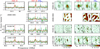 |
Fig. 1. IRAM PdBI and NOEMA spectra and images of CO(6–5), CO(7–6), and [C I] in quasar host galaxies at z ∼ 6. In the spectra, the dotted histograms mark the ±1σ range in the rms noise. The vertical red long-dashed and blue short-dashed lines mark the expected frequencies of the CO and [C I] transitions, respectively. The thick red lines show the best fit model of the spectra. In the right panels, the two continuum images were obtained by integrating over all of the line–free channels in the lower (1) and upper (2) side bands. The line maps are obtained by integrating over the observed or expected line width (see text for details). All the panels are 20″ × 20″ wide centered on the quasars. North is on the top, and east is on the left-hand side. Black and gray contours show the ±2,4,8,16-σ isophotes. The synthesized beam is shown as a white ellipse at the bottom left corner of the images. |
 |
Fig. 2. Continued from Fig. 1. In the last row, we show the stacked spectra of CO(6–5), CO(7–6) and [C I] obtained as described in Sect. 3.1. |
3. Results
In the following, we present our results on the spectral analysis of the new CO(7–6) + [C I] and CO(6–5) observations (Sect. 3.1). We then infer molecular gas mass estimates (Sect. 3.2), and constrain the properties of the ISM based on the available lines (Sect. 3.3).
3.1. Spectral analysis
We fit the 3 mm spectra from our sample and the 1 mm photometric measurements from the literature (see Table 1) with a Gaussian curve for each line: CO(6–5), CO(7–6), and [C I]; and a dust continuum described as:
![Mathematical equation: $$ \begin{aligned} S_{\nu , \mathrm {obs}}=\frac{\Omega }{(1+z)^3}\,[B_\nu (T_{\rm d})-B_\nu (T_{\rm CMB})]\,[1-\exp (-\tau _\nu )] \end{aligned} $$](/articles/aa/full_html/2022/06/aa42871-21/aa42871-21-eq11.gif) (1)
(1)
where Ω is the source angular size in steradiants; z is the source redshift; Bν(T) is the black body emissivity spectrum; Td is the dust temperature; TCMB is the CMB temperature at the source redshift, TCMB = 2.725 (1 + z) K. Finally, τν is the optical depth:
 (2)
(2)
where κd(ν) is the frequency–dependent dust absorption coefficient; Σd is the dust surface density; Md is the total dust mass within the angular size defined by Ω; DA is the angular diameter distance, DA = DL/(1 + z)2; NH2 is the column density of molecular gas; mH2 is the mass of the H2 molecule; and δg/d is the gas–to–dust mass ratio. We interpolate the κd(ν) values reported in Table 5 of Draine (2003) throughout the IR regime, and extrapolate assuming a power-law with slope β = 1.9 at ν < 350 GHz (see also da Cunha et al. 2021). At the CO(7–6) frequency, Eq. (2) implies that τν ∼ 1 for a molecular gas column density of ∼1.8 × 1025 cm−2 (assuming δg/d = 100, see, e.g., Berta et al. 2016). Such high column densities have been observed in the nuclei of some ULIRGs (e.g., Arp 220; see Scoville et al. 2017b), but are not expected to apply to the galaxy–averaged regimes sampled in our spatially unresolved observations (see also Sect. 3.3). At [C II] frequencies, the same optical depth is reached at ≈6.3× lower column densities.
We perform the spectral fits using our custom Monte Carlo Markov chain algorithm smc. We fit the redshift of the quasars, informed by the [C II] redshift; the width of the emission lines; the integrated fluxes of the lines; the dust continuum temperature, Td; and the dust mass within the beam, Md. Due to the modest signal-to-noise ratio of some of the lines in our survey, we impose that all of the fitted CO and [C I] lines of a given source have the same velocity width. As priors, we adopt Maxwellian distributions for the line width and the dust temperature (using 300 km s−1 and 50 K as scale lengths of the distributions); and loose Gaussian priors for the line fluxes and the logarithm of the dust mass. In Eqs. (1) and (2), we assume Ω = Ωbf, where Ωb is the resolution element in steradiants, and f is the (unconstrained) filling factor. Operatively, we assume f = 1 in the fits, and stress that, in the optically thin scenario, Ω has no impact on Sν and Md as it disappears from Eq. (1). The best fit and 1-σ errors on the fitted parameters are derived from the 50%, 14%, and 86% quantiles of the marginalized posterior distributions. The results of the fits are listed in Table 3. In the following, we treat as upper limits measurements of line fluxes and continuum flux densities for which the posterior flux estimates are below their upper 3-σ confidence level. All of the quasars are detected in the CO(7–6) emission line. Conversely, only 6/10 and 6/8 of the targeted quasars are detected in their [C I] and CO(6–5) emission, respectively.
Results from the spectral fits.
In Fig. 3, we plot the continuum flux density at 1 mm (at the rest frequency of [C II], as reported in the literature; see Table 1 for references) as a function of the observed flux densities at 3 mm [at the reference frequency of CO(7–6), from this work]. We find a typical 1 mm/3 mm flux density ratio of ∼19. Figure 3 also shows the flux densities expected under different assumptions of Td and τ1900 GHz, the optical depth τν computed at the [C II] frequency, for a quasar at z = 6, based on Eq. (2). The observed ratios favor relatively low optical depth values, τ1900 GHz ≲ 1 against the optically thick scenario (τ1900 GHz ≳ 5) for the quasars in our sample, unless extremely high temperatures (Td ≫ 100 K) are invoked. This suggests that the bulk of the dust is optically thin at 3 mm in these galaxy-wide observations, in contrast with what has been observed at the very center of some quasar host galaxies (e.g., Walter et al. 2022).
 |
Fig. 3. Measured continuum flux densities at 3 mm (at ν ≈ νCO(7−6)) and 1 mm (at ν ≈ ν[CII]). The expected flux density ratios for modified black body templates with different temperatures Td and opacity at the [C II] frequency, corrected for the CMB for a source at redshift z = 6, are shown for comparison. Our measurements, color-coded by the IR luminosity of the quasars, are generally consistent with Td = 47 K and τ1900 GHz = 0.2, or Td = 60 K and τ1900 GHz = 1. The former template is adopted in our analysis when computing IR luminosities and dust masses. |
For most of the quasars in our sample, only the two photometric points shown in Fig. 3 are available in the rest-frame far-infrared, thus making our estimates of the IR luminosities quite uncertain. In particular, the lack of constraints on the dust spectral energy distribution at wavelengths shorter than the expected peak hinders any informative constraints on the dust temperature, Td. For instance, the observed Fν(1 mm)/Fν(3 mm) ratios in our sample are equally fit with (Td,τ1900 GHz) = (60 K, 1) or (47 K, 0.2). With this caveat in mind, in the remainder of the analysis we infer IR luminosities following Eq. (2) under the assumption of τ1900 GHz = 0.2 and Td = 47 K, scaled to match the observed 1 mm flux density. These values are in line with the dust temperature reported for other high–z quasars that have been extensively studied in their dust spectral energy distribution (e.g., Beelen et al. 2006; Drouart et al. 2014; Leipski et al. 2014; Meyer et al. 2022). For the quasars J0338+0021, J2054–0005, and J1319+0950, we instead adopt the values published in Wang et al. (2013) and Leipski et al. (2014), based on the fits of their Spectral Energy Distributions. In all cases, the IR luminosities are computed by integrating the dust continuum between 8–1000 μm.
We convert line fluxes into luminosities, following, for instance, Carilli & Walter (2013):
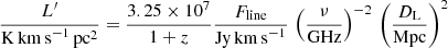 (3)
(3)
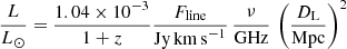 (4)
(4)
where Fline is the line integrated flux.
In Fig. 4, we compare the luminosity of the lines under examination with the infrared luminosity. Our sample spans a factor ∼10 in IR luminosity, but only a factor of ≲3 in the luminosity of any of the detected lines. Both the measured CO(6–5) and CO(7–6) luminosities are in line with empirical scaling relations based on local ULIRGs (see, e.g., Greve et al. 2014). This, together with the widespread detections of CO(7–6), and the similar luminosities found for CO(6–5) and CO(7–6), suggests that the CO excitation is relatively high up to Jup ≈ 7. We measure [C I] luminosities of (3−10)×107 L⊙, as expected based on the empirical [C I]–IR relation from Valentino et al. (2020). Finally, the [C II]/IR luminosity ratios in our sample span a factor ∼6, from 1.4 × 10⁻³ (J2219+0102) to 2.4 × 10⁻⁴ (J2054–0005), with lower [C II]/IR ratios typically observed for quasars with LIR > 3 × 10¹² L⊙ (see, e.g., Stacey et al. 2010; Gullberg et al. 2015). For comparison, the observed ratios in low and high surface density of star formation rate regimes as computed in Herrera-Camus et al. (2018) are [C II]/IR ≈ 1.6 × 10⁻³ and [C II]/IR ≈ 5 × 10⁻⁴, respectively (assuming the SFR–IR conversion from Kennicutt & Evans 2012).
 |
Fig. 4. Luminosity of CO(6–5), CO(7–6), [C I], and [C II], as a function of IR luminosity, for the quasars in our sample. For reference, we also show the CO line–IR luminosity relations from Greve et al. (2014) (dashed–dotted and long–dashed lines); the [C I]–LIR relation from Valentino et al. (2020) (solid line); and the two average values of the [C II]/IR luminosity ratio for low– and high–ΣIR galaxies from Herrera-Camus et al. (2018) (short dashed lines). The targeted quasars span a factor ∼10 in IR luminosity but only a factor ≳3 in each line luminosity. |
Capitalizing on the self-similarity of the line luminosities within our sample, we compute the average spectrum by shifting all of the 3 mm spectra to z = 6, and averaging the observed flux densities with weights set by the channel variance. The noise spectrum is derived as the sum of the inverse variance of the spectra of each source. We do not rescale the spectra based on the source luminosity. The stacked spectrum is then fitted in the similar fashion as individual sources. The stacked spectrum and the fitted values are reported in Fig. 2 and Table 3. In the following, when comparing the luminosity of the stacked lines with the one of [C II], for the stack we adopt the median luminosity of [C II] in our sample, L[CII] = 2.5 × 10⁹ L⊙.
3.2. Molecular gas masses
Here we infer molecular mass estimates via four recipes, based on the dust continuum emission and different molecular gas tracers. This allows us to test the consistency of the various mass estimators and to study the impact of working assumptions.
First, we derive the dust mass from the dust continuum emission. As discussed in the previous section, τν ≪ 1 at 3 mm in our galaxy–scale observations. In this regime, the dust is optically thin and Eq. (1) yields a nearly linear dependence of the observed flux density on τν, and hence, on the dust mass. In the following, we adopt the template used for the estimate of the IR luminosiy (Td = 47 K, τ1900 GHz = 0.2). Because the optical depth is fixed, Eq. (1) implies a constraint on the size of the emitting region, Ω, which thus sets the dust mass via Eq. (2). In this framework, an observed 3 mm flux density of 0.1 mJy for a source at z = 6 corresponds to a size of 0.097 arcsec2 (∼3.2 kpc2), and a dust mass of Md = 2.8 × 10⁸ M⊙. Our CO(7–6) observations have a median beam area of 16.8 arcsec2, yielding a typical filling factor f = 5.8 × 10⁻³. If instead we leave τν free, the dependence on the angular size is lost in the optically thin regime, and the flux density is simply a function of temperature and dust mass. As discussed in Sect. 3.1, however, we cannot constrain the dust temperature in the majority of our sample. If we refer to the best–fit values from our continuum fits, Td = 30–110 K, the inferred dust masses differ from the fiducial ones by an average factor ∼1.6. We convert the dust mass into the associated molecular gas mass via a gas–to–dust ratio, δg/d = 100 (see, e.g., Bolatto et al. 2013; Sandstrom et al. 2013; Genzel et al. 2015; Berta et al. 2016). For comparison, the analysis by Dunne et al. (2021) led to a mean value of δg/d = 128 ± 16, in broad agreement with the round value assumed here. The inferred molecular gas masses are listed in Table 4.
Inferred quantities from the observed line and continuum luminosities.
Molecular gas mass estimates in high–z galaxies typically rely on CO observations (see, e.g., reviews in Carilli & Walter 2013; Combes 2018; Tacconi et al. 2020; Hodge & da Cunha 2020). While low–J transitions should be preferred, as they are less sensitive to uncertainties on the CO excitation, the molecular mass estimates in z > 6 quasars tend to rely on intermediate (Jup = 5–7) transitions (e.g., Wang et al. 2010; Venemans et al. 2017a; Yang et al. 2019) which appear to be at the peak of the CO Spectral Line Energy Distribution for these quasars (e.g., Li et al. 2020). In this work, we pin our estimates to the CO(7–6) emission3. Molecular gas mass is derived from CO as:
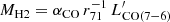 (5)
(5)
where we adopt a CO–to–H2 conversion factor αCO = 0.8 M⊙ (K km s−1 pc2)−1 typical for ULIRG and quasars (see discussions in Bolatto et al. 2013; Carilli & Walter 2013), and r71 is the CO(7–6)/CO(1–0) luminosity ratio, which we assume to be r71 = 0.17 based on the high–z CO excitation template in Boogaard et al. (2020). For comparison, the well-studied quasar J1148+5251 shows r71 > 0.12, and r73 = 0.58, suggesting very high CO excitation (Bertoldi et al. 2003; Riechers et al. 2009). Table 4 lists the inferred values.
A third path to molecular gas estimates capitalizes on the neutral carbon emission, which arises from the outer layers of molecular clouds as well as the diffuse molecular gas in the interstellar medium (see theoretical predictions in, e.g., Glover & Clark 2016; Clark et al. 2019; Bisbas et al. 2019; Galactic observations in, e.g., Frerking et al. 1989; Kramer et al. 2004; Cubick et al. 2008; Beuther et al. 2014; and searches at high redshift by, e.g., Walter et al. 2011; Alaghband-Zadeh et al. 2013; Bothwell et al. 2017; Popping et al. 2017; Papadopoulos et al. 2018; Valentino et al. 2018). In the optically thin assumption, following a three–level model of the carbon emission, the mass of neutral carbon can be inferred from the observed line luminosity using:
![Mathematical equation: $$ \begin{aligned} \frac{M_{\rm CI}}{M_\odot } = \frac{4.556}{10^{4}}\,\frac{Q_{\rm ex}}{5}\,\exp (62.5/T_{\rm ex})\,\frac{L^{\prime }_{\rm [CI]2-1}}{\mathrm{K\,km\,s}^{-1}\,\mathrm{pc}^2} \end{aligned} $$](/articles/aa/full_html/2022/06/aa42871-21/aa42871-21-eq138.gif) (6)
(6)
where Qex = 1 + 3 exp(−23.6/Tex)+5 exp(−62.5/Tex) is the partition function and Tex is the excitation temperature in Kelvin (see Weiß et al. 2003, 2005). We assume that the carbon emission is in thermal equilibrium with the dust, and thus adopt Tex = 47 K as measured on average in high–z quasars (Beelen et al. 2006; Leipski et al. 2014). The mass estimate in Eq. (6) is not very sensitive to Tex: any temperature in the range Tex = 30–100 K yields a mass estimate within ∼0.15 dex from our fiducial value. The resulting masses can be converted into H2 masses through the neutral carbon to H2 abundance, [C]/[H2], and accounting for the mass ratio of carbon atoms and H2 molecules. Following Boogaard et al. (2020), here we adopt a carbon abundance value of (1.9 ± 0.4)×10−5 (under the assumption that CO is in thermal equilibrium; see Bothwell et al. 2017; Boogaard et al. 2020). This value is consistent with the [C]/[H2] = (1.6 ± 0.1)×10−5 estimate by Dunne et al. (2021) for a sample of z = 0.35 galaxies.
Finally, recent work on intermediate redshift main sequence galaxies led to a definition of a molecular mass estimator based on [C II] (Zanella et al. 2018):
![Mathematical equation: $$ \begin{aligned} M_{\rm H2,[CII]} = \alpha _{\rm [CII]}\,L_{\rm [CII]}, \end{aligned} $$](/articles/aa/full_html/2022/06/aa42871-21/aa42871-21-eq139.gif) (7)
(7)
where L[CII] is the [C II] luminosity in solar units, and α[CII] ∼ 30 M⊙  is a scaling factor calibrated on a collection of main sequence and starburst galaxies. Venemans et al. (2017b) provide a first principle estimate of the ionized carbon mass in analogy to Eq. (6). Assuming Tex = 47 K, this formula is consistent with Eq. 7 if one assumes a [C+]/[H2] abundance of 3.4 × 10⁻⁵, that is, about 1.8 times higher than the [C]/[H2] abundance from Boogaard et al. (2020) but still in line with other carbon abundance values reported in the literature (e.g., Weiß et al. 2005). On the other hand, Sommovigo et al. (2021) find a wide range of α[CII] = 10–1000 for a sample of local galaxies, depending on the surface density of SFR and on the depletion time.
Figure 5 and Table 4 compare the molecular gas masses inferred with these four methods. All the MH2 estimates are in broad agreement, with typical values of 1010−11 M⊙, although the [C II]–based values show a systematic excess by ∼0.5 dex. Noticeably, Neeleman et al. (2021) find a similar excess for [C II]–based molecular gas mass measurements, when comparing to the dynamical masses obtained from high–resolution [C II] maps of quasars at similar redshifts. The dust–based estimates show the largest scatter in our work, as they spread over ∼1 dex; on the contrary, the CO–based estimates display a much smaller range (< 0.5 dex). The plot also highlights the impact of our operative assumptions: Our MH2 estimates depend linearly on αCO, δg/d, and α[CII], and antilinearly on r71, [C]/[H2], and (to first order) Td. Different assumptions for these parameters could mitigate or increase discrepancies among these mass estimates. For instance, by adopting a higher CO–to–H2 value, αCO = 3.6 M⊙ (K km s−1 pc2)−1 (see, e.g., Daddi et al. 2010), the CO–based estimates of MH2 would increase by a factor 4.5, thus narrowing the gap with respect to the [C II]–based ones, but at the same time separating them from the [C I]– and dust–based measurements. On the other hand, if we adopt a higher CO–excitation, for example, r71 = 0.38 from the quasar template in Carilli & Walter (2013) instead of the fiducial value r71 = 0.17 from Boogaard et al. (2020), we would reduce the CO–based dust mass estimates, thus widening the gap with respect to the [C II]–based estimates. Similarly, assuming a higher carbon abundance, [C]/[H2] = 5 × 10⁻⁵ as estimated by Weiß et al. (2005) in a sample of z ∼ 2.5 submillimeter galaxies, would yield a decrease in the [C I]–based mass of molecular gas. Along the same lines, one could adopt the method proposed by Sommovigo et al. (2021) to infer α[CII] and Td based on the surface brightness of [C II] for those quasars in our sample that have already been observed at high angular resolution in [C II] (PJ036+03, J1048–0109, J1319+0950, J2054–0005, and PJ359–06; see Venemans et al. 2020). The extremely high SFR densities reached in these sources lead to very low α[CII] ∼ 1 values and correspondingly to slightly higher dust temperatures, Td = 40–100 K. The higher Td would yield slightly lower (< 0.2 dex on average) MH2, dust estimates. However, the MH2, [CII] estimates would drop by a factor ∼30 based on this method, making them inconsistent with all other estimates. This discrepancy is likely due to the implicit wild extrapolation of local scaling relations (such as the Kennicutt–Schmidt star-formation law and the empirical SFR–L[CII] relation) toward regimes where other astrophysical mechanisms may be at play (for instance, [C II] might be suppressed by thermalization, changes in the photoelectric efficiency of dust grains, optical depth, and other processes; see e.g. Sutter et al. 2021). While a deeper understanding of the physical properties of the line and dust emitting ISM is required in order to directly constrain these unknown quantities, our analysis demonstrates that the fiducial values lead to consistent molecular gas mass estimates (within a factor ≲3).
 |
Fig. 5. Comparison between the mass estimates inferred from CO (MH2, CO), [C I] (MH2, [CI]), [C II] (MH2, [CII]) and dust continuum (MH2, dust), as described in the text. The one–to–one relation is shown as a dashed line. The different estimators lead to generally consistent results overall, with MH2 = 1010−11 M⊙, although different estimators lead to a different spread of values within our sample. The [C II]–based estimates are systematically higher than the ones based on other tracers. The arrows highlight how the data points would move if some parameters would change from their fiducial values to others commonly used in the literature. |
3.3. Physical properties of the cold ISM
In order to further explore the interplay among CO, [C I], [C II], and dust in high-z quasars, we assume that radiative processes (photodissociation, photoelectric heating, etc.) dominate over other nonradiative mechanisms altering the energy budget in the molecular gas (shocks, turbulence, cosmic rays, etc). This assumption allows us to directly compare our observations with the line and continuum luminosity predictions of Photo-Dissociation Regions (PDRs) and X-ray Dominated Regions (XDRs). The models are based on the analysis presented in Pensabene et al. (2021) and briefly summarized here. We use the CLOUDY radiative-transfer code (version c.17.01; Ferland et al. 2017) to predict the line emission of a single plane-parallel semi-infinite cloud impinged by a radiation field in both the PDR and XDR regimes. We created grids of 270 PDR and XDR models with total hydrogen density in the range log(nH [cm−3]) = [2, 6] (15 values in steps of ∼0.29 dex) and strength of the incident radiation field (18 models) in the range log G0 [Habing units] = [1, 6] (for PDRs), and log FX [erg s−1 cm−2] = [−2.0, 2.0] (for XDRs). We consider three cases of total hydrogen column density log NH [cm−2] = {22, 23, 24} (see Fig. 6). We assume that all the line emission arises from the neutral or molecular gas phase, in particular the contribution of HII regions to the [C II] emission is neglected (see, e.g., Díaz-Santos et al. 2017; Pensabene et al. 2021).
 |
Fig. 6. Luminosity line ratios predicted in the context of PDR and XDR models, as a function of column density, gas density, and strength of the incident radiation field (see text for details). The contours show the ratios measured in each source in our sample, color coded as shown in the legend. XDR models can reproduce the observed high [C II]/[C I] ratios only at low column densities, NH ≲ 1022 cm−2, whereas PDR models are compatible with the observed constraints over a wider range of parameters. The relatively low [C II]/CO(7–6) ratio observed in the targeted quasars is suggestive of typically large column densities, NH ≳ 1023 cm−2 for both PDR and XDR environments. Finally, the low observed [C I]/CO(7–6) ratios point to a high density nH ≳ 103 (105) cm−3 in PDRs (XDRs). Overall, a dense (nH > 103 cm−3) gas cloud with column densities of NH ∼ 1023 cm−2 impinged by UV radiation from newborn stars appears to best describe the observed line ratios. However, we stress that no single model accurately reproduces simultaneously all of the observed line ratios, thus suggesting that a single cloud is too simplistic a description of the observed phenomenology. |
The relative strength of all of the targeted lines is sensitive to the gas density, as well as to the intensity and hardness of the incident radiation field. For instance, the [C I]/CO(7–6) ratio is sensitive to the gas density in the regime nH < 104 cm−3, and only marginally affected by other parameters for NH ≳ 1023 cm−2. The [C II]/[C I] typically shows values > 10 in PDRs, while it is always < 10 in XDRs, unless NH ≲ 1022 cm−2. This is because X-rays penetrate deeper into the clouds than UV photons, thus heating the cloud cores and enhancing [C I]. For the same reason, CO molecules receive additional energy and thus the CO spectral line energy distribution shows stronger emission in the high–J transitions. This translates into a suppressed [C II]/CO(7–6) luminosity ratio in XDRs compared with predictions for PDRs, at least for high-density clouds (nH > 104 cm−3). At low column densities, NH ≲ 1022 cm−2, predictions for this set of observables based on PDR and XDR models tend to converge. The expected [C II]/[C I] ratios decrease in both models. Most notably, CO(7–6) emission is largely suppressed, thus leading to high [C II]/CO(7–6) and [C I]/CO(7–6) luminosity ratios.
As discussed in the previous sections, the line luminosities in our sample span a small range (< 0.5 dex). This implies that also the probed line ratios show similarly homogeneous values within the sample. We argue that the selection of IR–luminous (LIR > 1012 L⊙) sources might bias our sample toward a specific subclass of host galaxies hosting a compact starburst. In Fig. 6, we compare the predicted line ratios with the values observed for the quasars in our sample. We find that PDR models successfully predict the observed [C II]/[C I] ratios over a wide range of column densities. That is not the case for XDR models, which require low column densities in order to account for the high [C II]/[C I] luminosity ratios in our data. All models predict a wide range of [C II]/CO(7–6) luminosity ratios, although at low column densities it becomes increasingly difficult to explain the low values observed in our study, in particular if compared to predictions from PDR models. Finally, the observed [C I]/CO(7–6) luminosity ratios point to intermediate to high densities (nH ≳ 103 cm−3 in PDRs, nH ≳ 105 cm−3 in XDRs).
In Fig. 7, we compare the observed [C II]/[C I] and CO(7–6)/IR luminosity ratios in individual sources from our sample with other high-redshift quasars and SMGs (from Weiß et al. 2003, 2013; Riechers et al. 2009; Bradford et al. 2009; Ivison et al. 2010; Cox et al. 2011; De Breuck et al. 2011; Danielson et al. 2011; Wagg et al. 2012; Salomé et al. 2012; Walter et al. 2012; Riechers et al. 2013; Rawle et al. 2014; Leipski et al. 2014; Decarli et al. 2014; Venemans et al. 2017a; Yang et al. 2019; Zhao et al. 2020; Pensabene et al. 2021) as well local galaxies (based on the compilation in Rosenberg et al. 2015) and with the predictions from the models presented in Fig. 6. The quasars in our study appear to populate a rather narrow parameter space in this diagram: They all have [C II]/[C I] ≳ 20, consistent with most of the high-z sources in our comparison, as well as the bulk of the local sample from Rosenberg et al. (2015). Notably, only the local Seyfert 2 galaxy NGC 1068 falls (although, only marginally) in the [C II]/[C I] < 10 regime that is often adopted as a bona fide XDR domain. In terms of CO(7–6)/IR, we find values of 10−5 − 10−4, in line with most of the high–z comparison sample, and (on average) a factor 2–3 higher than most of the local galaxies in Rosenberg et al. (2015).
 |
Fig. 7. Observed [C II]/[C I] luminosity line ratio, as a function of the CO(7–6)/IR luminosity ratio (left panel), for the quasars in our study (filled circles; see references in the main text), as well as other high redshift (z > 1) galaxies and quasar hosts (filled squares) and local galaxies (empty stars, based on Rosenberg et al. 2015). All the quasars in our study show [C II]/[C I] ratios ≳20, which are not compatible with XDRs. Our sample also displays a range of CO(7–6)/IR ratios comparable with other high–z sources, but a factor ∼2−3× higher than the bulk of the local galaxies. Right: predictions of the [C II]/[C I] ratio as a function of the CO(7–6)/IR luminosity ratio for various gas densities log nH[cm−3] = (3, 4, 5) for a PDR with incident radiation field log G0 = (2, 3, 4) and an XDR with log FX = ( − 1, 0, +1). Our sources (shown in filled circled, with the same color scheme as in the left-hand panel) are best described by a PDR–like environment with NH ∼ 1023 cm−2, nH ≳ 104 cm−3, and G0 ∼ 103. |
In Fig. 7 we also show how the individual sources presented in our study compare with respect to the predicted [C II]/[C I] and CO(7–6)/IR luminosity ratios from our PDR and XDR models. As already mentioned, the high values observed for the [C II]/[C I] ratio point to a relatively low gas column density, NH ≲ 1023 cm−2 for PDRs, ≲1022 cm−2 for XDRs. However, at very low column densities, NH ∼ 1022 cm−2, the CO(7–6) luminosity is suppressed, thus models fail to reproduce the relatively high CO(7–6)/IR ratios observed in our quasars. The quasar population in our study appears to be best described by PDR models with column densities of NH ∼ 1023 cm−2, densities of nH ≳ 104 cm−3, impinged with a radiation field with G0 ∼ 103. These modest column density estimates are in agreement with the estimates based on the dust continuum slope discussed in Sect. 3.1. At face value, these constraints imply a line-of-sight thickness of the medium of only a few parsecs. However, we stress that the simplified models adopted here (in particular, because of the single-cloud treatment at fixed gas density, and because we neglect nonradiative ingredients contributing to the gas excitation, such as turbulence and cosmic rays) likely fail to capture the complex interplay of different phases in the ISM, thus these findings need to be taken with caution.
4. Conclusions
We present a survey of [C I], CO(7–6), CO(6–5) and their underlying dust continuum (observed at 3 mm) in a sample of ten quasar host galaxies at z ∼ 6. All of the quasars in our sample had previously been detected in their [C II] and dust continuum at ∼1 mm (in the observer’s frame). Our main findings are:
-
(i)
We detect CO(7–6) in all of the targeted quasars, and [C I] in 6 of them. Out of the 8 quasar host galaxies for which we have CO(6–5) coverage, we also report six detections in this emission line. The underlying 3 mm dust continuum is detected in 4/10 of the sample. This work doubles the number of z ∼ 6 quasars with CO(7–6) measurements in the literature.
-
(ii)
The observed flux density of the dust continuum emission at 3 mm and 1 mm is consistent with a modified black body emission with temperature Td = 47 K and an optical depth at the frequency of [C II] of τ1900 GHz = 0.2.
-
(iii)
Our targets span a factor ∼10 in IR luminosity, but only a factor ≲3 in the luminosity of any line detected in our study.
-
(iv)
We derive molecular gas masses using four independent methods, based on the dust continuum and the CO, [C I], and [C II] line emission. To first order, all the methods point to similar values of MH2 = 1010−11 M⊙. This confirms earlier results suggesting that immense gaseous reservoirs power the intense star formation and nuclear activity of the first quasar host galaxies. By combining the four independent measurements, we infer relative constraints on the unknown scaling factors (gas-to-dust, αCO, carbon abundance, α[CII], etc.). Our estimates for these conversion factors agree with the values inferred in a similar study by Dunne et al. (2021) on galaxies at z = 0.35.
-
(v)
We investigate the physical properties of the cold ISM via CLOUDY-based PDR and XDR models. By comparing the luminosity of dust, [C II], [C I], and CO(7–6), with the expectations from radiative transfer models, we find that the best (albeit imperfect) description of the observations requires a PDR–like environment with dense (nH > 104 cm−3) clouds impinged by a radiation field of G0 ∼ 103 (in Habing units). Column densities of NH ∼ 1023 cm−2 appear favored by our modeling, thus yielding a typical size of the clouds of only a few parsec.
This study confirms and further constrains the presence of massive reservoirs of molecular gas in the host galaxies of z ∼ 6 quasars, and suggests that star formation is the main mechanism responsible for the gas excitation at galactic scales. This work demonstrates the diagnostic power of combined 3 mm and 1 mm observations of very high-redshift sources, which can reveal a wide range of properties of the cold ISM in massive galaxies at cosmic dawn with only two frequency setups. Further NOEMA and ALMA observations will allow us to expand this analysis to a broader range of IR luminosities, and to extend the investigation to other sets of diagnostics (e.g., dense gas tracers, metallicity tracers, etc.).
For reference, SFR estimates based on a Chabrier (2003) initial mass function are practically unchanged, while adopting a Salpeter (1955) initial mass function would lead to ∼15% higher SFR estimates (Kennicutt & Evans 2012).
CO(7–6) is preferred to CO(6–5) as it is available for all of the sources, and in our dataset it usually displays higher signal-to-noise.
Acknowledgments
We are grateful to the referee for their useful and thorough report that helped to improve the manuscript. This work is based on observations carried out under project numbers S052, X04D, S15DA, S17CD, S18DM, S19DM with the IRAM NOEMA Interferometer. IRAM is supported by INSU/CNRS (France), MPG (Germany) and IGN (Spain). The research leading to these results has received funding from the European Union’s Horizon 2020 research and innovation program under grant agreement No 730562 [RadioNet]. R.D. is grateful to the IRAM staff and local contacts for their help and support in the data processing. F.W. and B.P.V. acknowledge support from ERC Advanced grant 740246 (Cosmic_Gas). D.R. acknowledges support from the National Science Foundation under grant numbers AST-1614213 and AST-1910107. D.R. also acknowledges support from the Alexander von Humboldt Foundation through a Humboldt Research Fellowship for Experienced Researchers. F.B. acknowledges support through the within the Collaborative Research Centre 956, sub-project A01, funded by the Deutsche Forschungsgemeinschaft (DFG) – project ID 184018867.
References
- Alaghband-Zadeh, S., Chapman, S. C., Swinbank, A. M., et al. 2013, MNRAS, 435, 1493 [Google Scholar]
- Bañados, E., Decarli, R., Walter, F., et al. 2015, ApJ, 805, L8 [CrossRef] [Google Scholar]
- Bañados, E., Venemans, B. P., Mazzucchelli, C., et al. 2018, Nature, 553, 473 [Google Scholar]
- Beelen, A., Cox, P., Benford, D. J., et al. 2006, ApJ, 642, 694 [NASA ADS] [CrossRef] [Google Scholar]
- Berta, S., Lutz, D., Genzel, R., Förster-Schreiber, N. M., & Tacconi, L. J. 2016, A&A, 587, A73 [NASA ADS] [CrossRef] [EDP Sciences] [Google Scholar]
- Bertoldi, F., Carilli, C. L., Cox, P., et al. 2003, A&A, 406, L55 [NASA ADS] [CrossRef] [EDP Sciences] [Google Scholar]
- Beuther, H., Ragan, S. E., Ossenkopf, V., et al. 2014, A&A, 571, A53 [NASA ADS] [CrossRef] [EDP Sciences] [Google Scholar]
- Bisbas, T. G., Schruba, A., & van Dishoeck, E. F. 2019, MNRAS, 485, 3097 [NASA ADS] [Google Scholar]
- Bolatto, A. D., Wolfire, M., & Leroy, A. K. 2013, ARA&A, 51, 207 [CrossRef] [Google Scholar]
- Boogaard, L. A., van der Werf, P., Weiss, A., et al. 2020, ApJ, 902, 109 [NASA ADS] [CrossRef] [Google Scholar]
- Bothwell, M. S., Aguirre, J. E., Aravena, M., et al. 2017, MNRAS, 466, 2825 [Google Scholar]
- Bradford, C. M., Aguirre, J. E., Aikin, R., et al. 2009, ApJ, 705, 112 [NASA ADS] [CrossRef] [Google Scholar]
- Carilli, C. L., & Walter, F. 2013, ARA&A, 51, 105 [NASA ADS] [CrossRef] [Google Scholar]
- Chabrier, G. 2003, PASP, 115, 763 [Google Scholar]
- Clark, P. C., Glover, S. C. O., Ragan, S. E., & Duarte-Cabral, A. 2019, MNRAS, 486, 4622 [Google Scholar]
- Combes, F. 2018, A&ARv, 26, 5 [NASA ADS] [CrossRef] [Google Scholar]
- Cox, P., Krips, M., Neri, R., et al. 2011, ApJ, 740, 63 [NASA ADS] [CrossRef] [Google Scholar]
- Cubick, M., Stutzki, J., Ossenkopf, V., Kramer, C., & Röllig, M. 2008, A&A, 488, 623 [NASA ADS] [CrossRef] [EDP Sciences] [Google Scholar]
- da Cunha, E., Hodge, J. A., Casey, C. M., et al. 2021, ApJ, 919, 30 [NASA ADS] [CrossRef] [Google Scholar]
- Daddi, E., Bournaud, F., Walter, F., et al. 2010, ApJ, 713, 686 [NASA ADS] [CrossRef] [Google Scholar]
- Danielson, A. L. R., Swinbank, A. M., Smail, I., et al. 2011, MNRAS, 410, 1687 [NASA ADS] [Google Scholar]
- De Breuck, C., Maiolino, R., Caselli, P., et al. 2011, A&A, 530, L8 [NASA ADS] [CrossRef] [EDP Sciences] [Google Scholar]
- De Rosa, G., Venemans, B. P., Decarli, R., et al. 2014, ApJ, 790, 145 [Google Scholar]
- Decarli, R., Walter, F., Carilli, C., et al. 2014, ApJ, 782, 78 [NASA ADS] [CrossRef] [Google Scholar]
- Decarli, R., Walter, F., Venemans, B. P., et al. 2017, Nature, 545, 457 [Google Scholar]
- Decarli, R., Walter, F., Venemans, B. P., et al. 2018, ApJ, 854, 97 [Google Scholar]
- Decarli, R., Dotti, M., Bañados, E., et al. 2019, ApJ, 880, 157 [Google Scholar]
- Díaz-Santos, T., Armus, L., Charmandaris, V., et al. 2017, ApJ, 846, 32 [Google Scholar]
- Drake, A. B., Farina, E. P., Neeleman, M., et al. 2019, ApJ, 881, 131 [CrossRef] [Google Scholar]
- Draine, B. T. 2003, ARA&A, 41, 241 [NASA ADS] [CrossRef] [Google Scholar]
- Drouart, G., De Breuck, C., Vernet, J., et al. 2014, A&A, 566, A53 [NASA ADS] [CrossRef] [EDP Sciences] [Google Scholar]
- Dunne, L., Maddox, S. J., Vlahakis, C., & Gomez, H. L. 2021, MNRAS, 501, 2573 [NASA ADS] [CrossRef] [Google Scholar]
- Farina, E. P., Arrigoni-Battaia, F., Costa, T., et al. 2019, ApJ, 887, 196 [Google Scholar]
- Fabian, A. 2012, ARA&A, 50, 455 [CrossRef] [Google Scholar]
- Fan, X., White, R. L., Davis, M., et al. 2000, AJ, 120, 1167 [NASA ADS] [CrossRef] [Google Scholar]
- Fan, X., Strauss, M. A., Schneider, D. P., et al. 2003, AJ, 125, 1649 [Google Scholar]
- Ferland, G. J., Chatzikos, M., Guzmán, F., et al. 2017, RMxAA, 53, 385 [NASA ADS] [Google Scholar]
- Frerking, M. A., Keene, J., Blake, G. A., & Phillips, T. G. 1989, ApJ, 344, 311 [Google Scholar]
- Genzel, R., Tacconi, L. J., Lutz, D., et al. 2015, ApJ, 800, 20 [Google Scholar]
- Goicoechea, J. R., Santa-Maria, M. G., Bron, E., et al. 2019, A&A, 622, A91 [NASA ADS] [CrossRef] [EDP Sciences] [Google Scholar]
- Glover, S. C. O., & Clark, P. C. 2016, MNRAS, 456, 3596 [Google Scholar]
- Greve, T. R., Leonidaki, I., Xilouris, E. M., et al. 2014, ApJ, 794, 142 [NASA ADS] [CrossRef] [Google Scholar]
- Groves, B. A., Schinnerer, E., Leroy, A., et al. 2015, ApJ, 799, 96 [Google Scholar]
- Gullberg, B., De Breuck, C., Vieira, J. D., et al. 2015, MNRAS, 449, 2883 [Google Scholar]
- Heckman, T. M., & Best, P. N. 2014, ARA&A, 52, 589 [Google Scholar]
- Herrera-Camus, R., Sturm, E., Graciá-Carpio, J., et al. 2018, ApJ, 861, 95 [Google Scholar]
- Hodge, J. A., & da Cunha, E. 2020, Roy. Soc. Open Sci., 7, 200556 [NASA ADS] [CrossRef] [Google Scholar]
- Ivison, R. J., Swinbank, A. M., Swinyard, B., et al. 2010, A&A, 518, L35 [NASA ADS] [CrossRef] [EDP Sciences] [Google Scholar]
- Kennicutt, R. C., & Evans, N. J. 2012, ARA&A, 50, 531 [NASA ADS] [CrossRef] [Google Scholar]
- King, A., & Pounds, K. 2015, ARA&A, 53, 115 [NASA ADS] [CrossRef] [Google Scholar]
- Kramer, C., Jakob, H., Mookerjea, B., et al. 2004, A&A, 424, 887 [NASA ADS] [CrossRef] [EDP Sciences] [Google Scholar]
- Leipski, C., Meisenheimer, K., Walter, F., et al. 2014, ApJ, 785, 154 [Google Scholar]
- Li, J., Wang, R., Riechers, D., et al. 2020, ApJ, 889, 162 [NASA ADS] [CrossRef] [Google Scholar]
- Maloney, P. R., Hollenbach, D. J., & Tielens, A. G. G. M. 1996, ApJ, 466, 561 [Google Scholar]
- Mazzucchelli, C., Bañados, E., Venemans, B. P., et al. 2017, ApJ, 849, 91 [Google Scholar]
- Meijerink, R., Spaans, M., & Israel, F. P. 2007, A&A, 461, 793 [NASA ADS] [CrossRef] [EDP Sciences] [Google Scholar]
- Meyer, R. A., et al. 2022, ApJ, submitted [Google Scholar]
- Neeleman, M., Novak, M., Venemans, B. P., et al. 2021, ApJ, 911, 141 [NASA ADS] [CrossRef] [Google Scholar]
- Novak, M., Bañados, E., Decarli, R., et al. 2019, ApJ, 881, 63 [NASA ADS] [CrossRef] [Google Scholar]
- Papadopoulos, P. P., Bisbas, T. G., & Zhang, Z.-Y. 2018, MNRAS, 478, 1716 [NASA ADS] [CrossRef] [Google Scholar]
- Pensabene, A., Decarli, R., Bañados, E., et al. 2021, A&A, 652, A66 [NASA ADS] [CrossRef] [EDP Sciences] [Google Scholar]
- Popping, G., Decarli, R., Man, A. W. S., et al. 2017, A&A, 602, A11 [NASA ADS] [CrossRef] [EDP Sciences] [Google Scholar]
- Rawle, T. D., Egami, E., Bussmann, R. S., et al. 2014, ApJ, 783, 59 [NASA ADS] [CrossRef] [Google Scholar]
- Riechers, D. A., Walter, F., Bertoldi, F., et al. 2009, ApJ, 703, 1338 [NASA ADS] [CrossRef] [Google Scholar]
- Riechers, D. A., Bradford, C. M., Clements, D. L., et al. 2013, Nature, 496, 329 [Google Scholar]
- Rosenberg, M. J. F., van der Werf, P. P., Aalto, S., et al. 2015, ApJ, 801, 72 [Google Scholar]
- Salomé, P., Guélin, M., Downes, D., et al. 2012, A&A, 545, A57 [NASA ADS] [CrossRef] [EDP Sciences] [Google Scholar]
- Salpeter, E. E. 1955, ApJ, 121, 161 [Google Scholar]
- Sandstrom, K. M., Leroy, A. K., Walter, F., et al. 2013, ApJ, 777, 5 [Google Scholar]
- Schindler, J.-T., Farina, E. P., Bañados, E., et al. 2020, ApJ, 905, 51 [Google Scholar]
- Scoville, N., Lee, N., Vanden, Bout P., et al. 2017a, ApJ, 837, 150 [NASA ADS] [CrossRef] [Google Scholar]
- Scoville, N., Murchikova, L., Walter, F., et al. 2017b, ApJ, 836, 665 [NASA ADS] [Google Scholar]
- Somerville, R. S., & Davé, R. 2015, ARA&A, 53, 51 [Google Scholar]
- Sommovigo, L., Ferrara, A., Carniani, S., et al. 2021, MNRAS, 503, 4878 [NASA ADS] [CrossRef] [Google Scholar]
- Sommovigo, L., Ferrara, A., Pallottini, A., et al. 2022, MNRAS, in press [Google Scholar]
- Stacey, G. J., Hailey-Dunsheath, S., Ferkinhoff, C., et al. 2010, ApJ, 724, 957 [NASA ADS] [CrossRef] [Google Scholar]
- Sutter, J., Dale, D. A., Sandstrom, K., et al. 2021, MNRAS, 503, 911 [NASA ADS] [CrossRef] [Google Scholar]
- Tacconi, L. J., Genzel, R., & Sternberg, A. 2020, ARA&A, 58, 157 [NASA ADS] [CrossRef] [Google Scholar]
- Tielens, A. G. G. M., & Hollenbach, D. 1985, ApJ, 291, 722 [Google Scholar]
- Trakhtenbrot, B., Lira, P., Netzer, H., et al. 2017, ApJ, 836, 8 [NASA ADS] [CrossRef] [Google Scholar]
- Valentino, F., Magdis, G. E., Daddi, E., et al. 2018, ApJ, 869, 27 [Google Scholar]
- Valentino, F., Magdis, G. E., Daddi, E., et al. 2020, ApJ, 890, 24 [Google Scholar]
- Vallini, L., Tielens, A. G. G. M., Pallottini, A., et al. 2019, MNRAS, 490, 4502 [CrossRef] [Google Scholar]
- Venemans, B. P., Walter, F., Decarli, R., et al. 2017a, ApJ, 845, 154 [Google Scholar]
- Venemans, B. P., Walter, F., Decarli, R., et al. 2017b, ApJ, 851, L8 [NASA ADS] [CrossRef] [Google Scholar]
- Venemans, B. P., Decarli, R., Walter, F., et al. 2018, ApJ, 866, 159 [Google Scholar]
- Venemans, B. P., Walter, F., Neeleman, M., et al. 2020, ApJ, 904, 130 [Google Scholar]
- Vito, F., Brandt, W. N., Bauer, F. E., et al. 2019, A&A, 628, L6 [NASA ADS] [CrossRef] [EDP Sciences] [Google Scholar]
- Wagg, J., Wiklind, T., Carilli, C. L., et al. 2012, ApJ, 752, L30 [NASA ADS] [CrossRef] [Google Scholar]
- Walter, F., Bertoldi, F., Carilli, C., et al. 2003, Nature, 424, 406 [Google Scholar]
- Walter, F., Weiss, A., Downes, D., Decarli, R., & Henkel, C. 2011, ApJ, 730, 18 [NASA ADS] [CrossRef] [Google Scholar]
- Walter, F., Decarli, R., Carilli, C., et al. 2012, Nature, 486, 233 [Google Scholar]
- Walter, F., Neeleman, M., Decarli, R., et al. 2022, ApJ, 927, 21 [NASA ADS] [CrossRef] [Google Scholar]
- Wang, R., Wagg, J., Carilli, C. L., et al. 2008a, AJ, 135, 1201 [NASA ADS] [CrossRef] [Google Scholar]
- Wang, R., Carilli, C. L., Wagg, J., et al. 2008b, ApJ, 687, 848 [NASA ADS] [CrossRef] [Google Scholar]
- Wang, R., Carilli, C. L., Neri, R., et al. 2010, ApJ, 714, 699 [Google Scholar]
- Wang, R., Wagg, J., Carilli, C. L., et al. 2011, AJ, 142, 101 [NASA ADS] [CrossRef] [Google Scholar]
- Wang, R., Wagg, J., Carilli, C. L., et al. 2013, ApJ, 773, 44 [Google Scholar]
- Wang, F., Wang, R., Fan, X., et al. 2019, ApJ, 880, 2 [NASA ADS] [CrossRef] [Google Scholar]
- Wang, F., Yang, J., Fan, X., et al. 2021, ApJ, 907, L1 [Google Scholar]
- Weiß, A., Henkel, C., Downes, D., & Walter, F. 2003, A&A, 409, L41 [NASA ADS] [CrossRef] [EDP Sciences] [Google Scholar]
- Weiß, A., Downes, D., Henkel, C., & Walter, F. 2005, A&A, 429, L25 [NASA ADS] [CrossRef] [EDP Sciences] [Google Scholar]
- Weiß, A., De Breuck, C., Marrone, D. P., et al. 2013, ApJ, 767, 88 [Google Scholar]
- Willott, C. J., Bergeron, J., & Omont, A. 2017, ApJ, 850, 108 [Google Scholar]
- Yang, J., Venemans, B., Wang, F., et al. 2019, ApJ, 880, 153 [NASA ADS] [CrossRef] [Google Scholar]
- Yang, J., Wang, F., Fan, X., et al. 2020, ApJ, 897, L14 [Google Scholar]
- Yang, J., Wang, F., Fan, X., et al. 2021, ApJ, 923, 262 [NASA ADS] [CrossRef] [Google Scholar]
- Zanella, A., Daddi, E., Magdis, G., et al. 2018, MNRAS, 481, 1976 [Google Scholar]
- Zhao, Y., Lu, N., Díaz-Santos, T., et al. 2020, ApJ, 892, 145 [NASA ADS] [CrossRef] [Google Scholar]
All Tables
All Figures
|
Fig. 1. IRAM PdBI and NOEMA spectra and images of CO(6–5), CO(7–6), and [C I] in quasar host galaxies at z ∼ 6. In the spectra, the dotted histograms mark the ±1σ range in the rms noise. The vertical red long-dashed and blue short-dashed lines mark the expected frequencies of the CO and [C I] transitions, respectively. The thick red lines show the best fit model of the spectra. In the right panels, the two continuum images were obtained by integrating over all of the line–free channels in the lower (1) and upper (2) side bands. The line maps are obtained by integrating over the observed or expected line width (see text for details). All the panels are 20″ × 20″ wide centered on the quasars. North is on the top, and east is on the left-hand side. Black and gray contours show the ±2,4,8,16-σ isophotes. The synthesized beam is shown as a white ellipse at the bottom left corner of the images. |
| In the text | |
|
Fig. 2. Continued from Fig. 1. In the last row, we show the stacked spectra of CO(6–5), CO(7–6) and [C I] obtained as described in Sect. 3.1. |
| In the text | |
|
Fig. 3. Measured continuum flux densities at 3 mm (at ν ≈ νCO(7−6)) and 1 mm (at ν ≈ ν[CII]). The expected flux density ratios for modified black body templates with different temperatures Td and opacity at the [C II] frequency, corrected for the CMB for a source at redshift z = 6, are shown for comparison. Our measurements, color-coded by the IR luminosity of the quasars, are generally consistent with Td = 47 K and τ1900 GHz = 0.2, or Td = 60 K and τ1900 GHz = 1. The former template is adopted in our analysis when computing IR luminosities and dust masses. |
| In the text | |
|
Fig. 4. Luminosity of CO(6–5), CO(7–6), [C I], and [C II], as a function of IR luminosity, for the quasars in our sample. For reference, we also show the CO line–IR luminosity relations from Greve et al. (2014) (dashed–dotted and long–dashed lines); the [C I]–LIR relation from Valentino et al. (2020) (solid line); and the two average values of the [C II]/IR luminosity ratio for low– and high–ΣIR galaxies from Herrera-Camus et al. (2018) (short dashed lines). The targeted quasars span a factor ∼10 in IR luminosity but only a factor ≳3 in each line luminosity. |
| In the text | |
|
Fig. 5. Comparison between the mass estimates inferred from CO (MH2, CO), [C I] (MH2, [CI]), [C II] (MH2, [CII]) and dust continuum (MH2, dust), as described in the text. The one–to–one relation is shown as a dashed line. The different estimators lead to generally consistent results overall, with MH2 = 1010−11 M⊙, although different estimators lead to a different spread of values within our sample. The [C II]–based estimates are systematically higher than the ones based on other tracers. The arrows highlight how the data points would move if some parameters would change from their fiducial values to others commonly used in the literature. |
| In the text | |
|
Fig. 6. Luminosity line ratios predicted in the context of PDR and XDR models, as a function of column density, gas density, and strength of the incident radiation field (see text for details). The contours show the ratios measured in each source in our sample, color coded as shown in the legend. XDR models can reproduce the observed high [C II]/[C I] ratios only at low column densities, NH ≲ 1022 cm−2, whereas PDR models are compatible with the observed constraints over a wider range of parameters. The relatively low [C II]/CO(7–6) ratio observed in the targeted quasars is suggestive of typically large column densities, NH ≳ 1023 cm−2 for both PDR and XDR environments. Finally, the low observed [C I]/CO(7–6) ratios point to a high density nH ≳ 103 (105) cm−3 in PDRs (XDRs). Overall, a dense (nH > 103 cm−3) gas cloud with column densities of NH ∼ 1023 cm−2 impinged by UV radiation from newborn stars appears to best describe the observed line ratios. However, we stress that no single model accurately reproduces simultaneously all of the observed line ratios, thus suggesting that a single cloud is too simplistic a description of the observed phenomenology. |
| In the text | |
|
Fig. 7. Observed [C II]/[C I] luminosity line ratio, as a function of the CO(7–6)/IR luminosity ratio (left panel), for the quasars in our study (filled circles; see references in the main text), as well as other high redshift (z > 1) galaxies and quasar hosts (filled squares) and local galaxies (empty stars, based on Rosenberg et al. 2015). All the quasars in our study show [C II]/[C I] ratios ≳20, which are not compatible with XDRs. Our sample also displays a range of CO(7–6)/IR ratios comparable with other high–z sources, but a factor ∼2−3× higher than the bulk of the local galaxies. Right: predictions of the [C II]/[C I] ratio as a function of the CO(7–6)/IR luminosity ratio for various gas densities log nH[cm−3] = (3, 4, 5) for a PDR with incident radiation field log G0 = (2, 3, 4) and an XDR with log FX = ( − 1, 0, +1). Our sources (shown in filled circled, with the same color scheme as in the left-hand panel) are best described by a PDR–like environment with NH ∼ 1023 cm−2, nH ≳ 104 cm−3, and G0 ∼ 103. |
| In the text | |
Current usage metrics show cumulative count of Article Views (full-text article views including HTML views, PDF and ePub downloads, according to the available data) and Abstracts Views on Vision4Press platform.
Data correspond to usage on the plateform after 2015. The current usage metrics is available 48-96 hours after online publication and is updated daily on week days.
Initial download of the metrics may take a while.