| Issue |
A&A
Volume 661, May 2022
|
|
|---|---|---|
| Article Number | A135 | |
| Number of page(s) | 19 | |
| Section | Extragalactic astronomy | |
| DOI | https://doi.org/10.1051/0004-6361/202142358 | |
| Published online | 19 May 2022 | |
Physical model for the broadband energy spectrum of X-ray illuminated accretion discs: Fitting the spectral energy distribution of NGC 5548
1
Astronomical Institute of the Czech Academy of Sciences, Boční II 1401, 14100 Prague, Czech Republic
e-mail: michal.dovciak@asu.cas.cz
2
Department of Physics and Institute of Theoretical and Computational Physics, University of Crete, 71003 Heraklion, Greece
3
Institute of Astrophysics, FORTH, 71110 Heraklion, Greece
4
IRAP, Université de Toulouse, CNRS, UPS, CNES 9, Avenue du Colonel Roche, BP 44346, 31028 Toulouse Cedex 4, France
5
National Astronomical Observatories, Chinese Academy of Sciences, 20A Datun Road, Beijing 100101, PR China
Received:
3
October
2021
Accepted:
21
January
2022
Aims. We develop a new physical model for the broadband spectral energy distribution (SED) of X-ray illuminated accretion discs that takes into account the mutual interaction of the accretion disc and the X-ray corona, including all the relativistic effects induced by the strong gravity of the central black hole (BH) on light propagation and on the transformation of the photon energy, from the disc to or from the corona rest-frames, and to the observer.
Methods. We assumed a Keplerian optically thick and geometrically thin accretion disc and an X-ray source in the lamp-post geometry. The X-ray corona emits an isotropic, power-law-like X-ray spectrum, with a high-energy cut-off. We also assumed that all the energy that would be released by thermal radiation in the standard disc model in its innermost part is transported to the corona, effectively cooling the disc in this region. In addition, we include the disc heating due to thermalisation of the absorbed part of the disc illumination by the X-ray source. X-ray reflection due to the disc illumination is also included. The X-ray luminosity is given by the energy extracted from the accretion disc (or an external source) and the energy brought by the scattered photons themselves, thus energy balance is preserved. We computed the low-energy X-ray cut-off through an iterative process, taking full account of the interplay between the X-ray illumination of the disc and the resulting accretion disc spectrum that enters the corona. We also computed the corona radius, taking the conservation of the photon number during Comptonisation into account.
Results. We discuss in detail the model SEDs and their dependence on the parameters of the system. We show that the disc-corona interaction has profound effects on the resultant SED, it constrains the X-ray luminosity and changes the shape and normalisation of the UV blue bump. We also compare the model SEDs with those predicted from similar models currently available. We use the new code to fit the broadband SED of NGC 5548, which is a typical Seyfert 1 galaxy. When combined with the results from previous model fits to the optical and UV time-lags of the same source, we infer a high black-hole spin, an intermediate system inclination, and an accretion rate below 10% of Eddington. The X-ray luminosity in this source could be supported by 45–70% of the accretion energy dissipated in the disc. The new model, named KYNSED, is publicly available to be used for fitting AGN SEDs inside the XSPEC spectral analysis tool.
Conclusions. X-ray illumination of the accretion disc in AGN can explain both the observed UV and optical time-lags and the broadband SED of at least one AGN, namely NGC 5548. A simultaneous study of the optical, UV, and X-ray spectral and timing properties of these AGN with multiwavelength, long monitoring observations in the past few years will allow us to investigate the X-ray and disc geometry in these systems, and to constrain their physical parameters.
Key words: accretion, accretion disks / galaxies: active / galaxies: Seyfert
© ESO 2022
1. Introduction
It is widely accepted that active galactic nuclei (AGN) are powered by accretion of matter onto a supermassive BH. The modesl of Shakura & Sunyaev (1973, hereafter SS73) and Novikov et al. (1973, hereafter NT73) are the standard accretion disc models that have been extensively used to study the accretion process in these objects. These models cannot account for the copious emission of X-rays from AGN. Somehow, through an as yet unknown mechanism, accretion power is released into a region in which electrons are heated, and they then up-scatter the ultraviolet (UV) and optical photons emitted by the disc to X-rays. This region is also known as the X-ray corona.
The size and location of the corona are not known at the moment. X-ray monitoring of several lensed quasars has shown that the half-light radius of the X-ray source is smaller than a few dozen gravitational radii (e.g. see Fig. 1 in Chartas et al. 2016). The corona is probably located close to the BH, where most of the accretion power is released. Further information regarding its location with respect to the accretion disc is provided by X-ray spectroscopy.
More than thirty years ago, GINGA observations showed that a strong fluorescent iron Kα emission line and a considerable flattening of the X-ray continuum at energies higher than ∼10 keV were common features in the X-ray spectra of bright Seyferts (e.g. Nandra et al. 1991). Both features were interpreted as evidence for reprocessing of the X-ray continuum by a slab of cold and dense gas (e.g. Pounds et al. 1990; George & Fabian 1991). If this were the accretion disc, then the X-rays would need to be located above the disc to be able to illuminate it.
This scenario makes one implicit prediction. As most of the X-rays will be absorbed, they will generate heat in the disc. As a result, the disc will emit thermal radiation at frequencies that will depend on its effective temperature. We therefore expect the thermally reprocessed radiation to emerge in the UV and optical part of the spectrum. Furthermore, because the X-rays are highly variable in AGN, we would expect the X-ray variations to be correlated with the UV and optical variations, with a delay that depends on the geometry and on the physical properties of the system (accretion rate, X-ray luminosity, etc.).
Many multiwavelength monitoring campaigns of nearby Seyferts have been performed in the past decades in order to study the correlation between the X-ray, UV and optical variations. The observational effort has significantly intensified in the past ten years. A few AGN have been observed continuously and intensively for many months over a wide range of spectral bands from the optical to X-rays (e.g. McHardy et al. 2014; Fausnaugh et al. 2016; Cackett et al. 2018, 2020; Edelson et al. 2019; Pahari et al. 2020; Hernández Santisteban et al. 2020; Vincentelli et al. 2021; Kara et al. 2021). In all cases, the UV and optical variations are well correlated, but with a delay that increases from the UV to the optical bands, as expected in the case of X-ray illumination of the disc. The dependence of the time-lags on the wavelength agrees with the predictions of the standard accretion disc models. However, the lag amplitude appeared to be larger than expected by a factor of ∼2 − 3, given the BH mass and accretion rate of the objects.
Recently, we studied in detail the response of a standard accretion disc in the UV and optical bands when it is illuminated by X-rays in the lamp-post geometry (Kammoun et al. 2021a, hereafter K21a). We considered all relativistic effects to determine the incident X-ray flux on the disc, and in propagating light from the source to the disc and to the observer. We computed the disc reflection flux taking the disc ionisation into consideration, we calculated the disc response for many model parameters, and we provided a model relation between the X-ray time-lags and the UV and optical time-lags that depends on the BH mass, accretion rate, the X-ray corona height, and the (observed) 2–10 keV band luminosity (for a BH spin of 0 and 1). Using this model, we showed that the observed UV and optical time-lags in AGN are fully consistent with the standard accretion disc model as long as the disc is illuminated by a corona that is located ∼30 − 40 rg above the BH (Kammoun et al. 2021b, hereafter K21b).
In this work, we present a new model that can be used to fit the broadband SED of AGN from optical and UV to X-rays. The model is based on the K21a model, with some important modifications. K21a considered the X-ray luminosity as a free parameter. In the new model, we also consider the possibility that through some physical mechanism, all the accretion power below a transition radius, rtrans, is transferred to the corona. In this way, a direct link between the disc and the X-ray corona is established. The X-ray luminosity is no longer a free parameter, but rather depends on the accretion rate and rtrans. In this respect, the model is similar to AGNSED, which is a model that can fit the broadband AGN SEDs. AGNSED was developed by Kubota & Done (2018), and it is an update of an earlier model by Done et al. (2012), called optxagnf. Apart from this similarity, there are also many differences between our model and AGNSED. We compare the two models in detail in Sect. 3.
The new model includes a better treatment for the determination of the low-energy cut-off in the X-ray spectrum, which is an important parameter for determining the X-ray flux incident on the disc (and hence the number of the X-rays that are absorbed and the importance of X-ray illumination), as well as the X-ray spectrum normalisation. It also considers conservation of the number of disc photons as they scatter off the hot electrons in the corona. In this way, the model determines the size of the X-ray corona. This should be compared with the height of the source, as the corona radius should be smaller than the corona height minus the horizon radius, at least. Any discrepancies indicate that the adopted lamp-post geometry is not consistent with the data.
In the second part of the paper, we present the results from the model fitting of the average broadband energy spectrum of NGC 5548. This was one of the first AGN that was simultaneously observed in the X-rays and in the UV with the aim to test whether the variations in these two bands are correlated (Clavel et al. 1992). It was also monitored by Swift, the Hubble Space Telescope (HST), and ground-based telescopes over long periods in the past few years (McHardy et al. 2014; Edelson et al. 2015). In Kammoun et al. (2019, K19, hereafter) and K21b, we fitted the observed time-lag spectra of the source reported by Fausnaugh et al. (2016), and we found a very good agreement with a standard disc that accretes at a few percent of the Eddington limit and is illuminated by an X-ray source located at a height of 20 − 60 or 30 − 80 rg, depending on whether the BH spin is 0 or 1. In addition, we also studied the X-ray, UV, and optical power spectra of the STORM light curves (Panagiotou et al. 2020). We used the disc response functions of K19, and we found that the amplitude of the UV and optical PSDs are also compatible with a standard disc that is illuminated by X-rays with low accretion rates.
The paper is organised as follows: in Sect. 2 we explain our assumptions and describe all the details of the model set-up, in Sect. 3 we show the broadband SED predicted by our model for different model parameter values, in Sect. 4 we apply the model to the broadband energy spectrum of NGC 5548, and in Sect. 5 we conclude by summing up our results.
2. Model set-up
We have already studied the disc thermal reverberation in K19, K21a, and K21b. K21a developed a code that can compute the disc response function for a given BH mass, accretion rate, X-ray luminosity, and so on. In this work, we present a new code, KYNSED, which can be used to fit the broadband SED of AGN from optical to hard X-rays. The model is similar to the model outlined in K21a, with some important modifications that we describe in the following sections.
We considered a Keplerian, geometrically thin, and optically thick accretion disc with an accretion rate of ṁEdd around a BH with a mass of MBH and spin a*. Note that ṁEdd is the accretion rate normalised to the Eddington accretion rate, that is, ṁEdd = Ṁ/ṀEdd, where Ṁ is the accretion rate in physical units, and ṀEdd is the accretion rate for the total disc luminosity to be equal to the Eddington luminosity. It depends on the accretion efficiency, that is, on the BH spin. The BH spin is defined as a* = Jc/G , where J is the angular momentum of the BH, and is smaller than or equal to 1, see for instance Misner et al. (1973). We assumed that the intrinsic disc temperature profile follows the NT73 prescription. We took the spectral hardening due to photon interactions with matter in the upper disc layers into account via a colour-correction factor, fcol, as described by Done et al. (2012). It depends on the effective temperature of the disc, hence on all parameters that determine the disc temperature (e.g. MBH, ṁEdd, and X-ray incident flux). Following Done et al. (2012), we assumed that fcol = 1 when Td(r) < 3 × 10⁴ K, then fcol = (Td(r)/3 × 104 K)0.82 over the critical temperature range of 3 × 10⁴ K < Td(r) < 105 K, and then fcol = (72 keV/kBTd(r))1/9 at higher disc temperatures (Td(r) is the disc temperature in kelvin, which is set by the energy released locally by the accretion process and by the X-ray absorbed flux, and kB = 8.62 × 10⁻⁸ keV K−1 is Boltzmann constant). The colour-correction factor changes the disc temperature and the normalisation of the emitted black-body radiation at each radius, r, in such a way that the total radiated power does not change.
As for the X-ray source, we assumed the lamp-post geometry: the X-ray corona is point-like and is located at a height h above the BH, on its rotational axis. We also assumed that the X-rays are emitted isotropically in the rest-frame of the corona. They illuminate the disc, which will increase its temperature due to the thermalisation of the absorbed incident flux.
As K21a showed (see e.g. their Eq. (4) ), the observed disc flux at a particular wavelength, Fobs(λ, t), will be equal to the NT disc flux, FNT(λ), plus an additional term due to the disc heating by the X-ray absorption,
The equation above assumes that the disc variability is due only to the (variable) X-ray illumination of the disc. The convolution in the right-hand side gives the thermally reprocessed disc emission. The term LX in K21a is equal to the observed 2 − 10 keV luminosity of the corona (in Eddington units). In general, it can be any quantity representative of the corona luminosity. For example, it can be the total X-ray luminosity itself, as long as the disc response is normalised accordingly. ΨLX(λ, t) is the disc response function at λ, which depends on the X-ray luminosity in a non-linear way (see K21a).
It is difficult to model the observed AGN SEDs using Eq. (1). If we were to use simultaneous observations to construct the optical and UV SED, we would need continuous X-ray observations over a long time in order to compute the convolution integral in the right part of Eq. (1). The duration of the X-ray observations depends on the X-ray variability amplitude of each source and on the width of the disc response function, which is wavelength dependent. For example, modelling the contemporaneous SED of an AGN with measurements from ∼1000 up to ∼10 000 Å will require continuous X-ray observations over ∼1 up to ∼20 − 30 days prior to the optical and UV observations to compute the convolution integral in Eq. (1) for the shortest and longest wavelength in the SED. Note that these numbers are indicative, and correspond to the time at which the respective disc response function decreases by a factor of a few as compared to its maximum value. The numbers correspond to the 1158 Å and the z-band disc response plotted in the top panel in Fig. 8 in K21a. They depend on the wavelength and on the considered model parameters.
Equation (1) can be used to study the time-averaged SED because
where brackets denote the mean. K21a showed (see their Appendix A) that even if X-rays vary by about a factor of ∼10, the integral in the right-hand side of Eq. (2) is almost equal to the product of the mean X-ray luminosity, ⟨LX⟩ and the integral of Ψ⟨LX⟩(t), that is, the response function that corresponds to ⟨LX⟩. In this case, Eq. (2) can be re-written as
KYNSED used this equation to compute the mean X-ray, UV and optical SED in AGN. We explain the model in the following sections in detail.
2.1. Transfer of the energy from the accretion disc to the corona
The power that heats the corona is a free parameter in K21a. In this work, we also considered the possibility that the power from the accretion flow that is used to heat the gas below a transition radius, rtrans, is transferred to the corona by an unknown physical mechanism (i.e. similarly as was done in AGNSED, see Kubota & Done 2018). In this way, the luminosity of the X-ray source is no longer a free parameter: rtrans determines the total luminosity of the corona. The transition radius, rtrans, as well as all other radii, is measured with respect to the gravitational radius, rg = G MBH/c2.
We also assumed that the accretion disc is still Keplerian below rtrans, with an unchanged radial transfer of energy and angular momentum. If the power that is transferred to the corona, Ltransf, is equal to the disc luminosity (at infinity) emitted below the transition radius, then
![$$ \begin{aligned} L_{\rm transf}=2\pi \int _{r_{\rm ms}}^{r_{\rm trans}}\,\sigma T^4_{\rm NT}(r) [-U_t(r)]\,r\,\mathrm{d}r, \end{aligned} $$](/articles/aa/full_html/2022/05/aa42358-21/aa42358-21-eq5.gif)
where rms is the radius of the marginally stable orbit (also referred to as the radius of the innermost circular stable orbit, ISCO, rISCO), −Ut(r) is the time component of the accretion disc four-velocity that transforms the locally released accretion energy into the one with respect to the observer at infinity, and TNT(r) is the radially dependent NT73 effective disc temperature. The integral of the equation above over the whole accretion disc gives the total disc luminosity,
![$$ \begin{aligned} L_{\rm disc}=2\pi \int _{r_{\rm ms}}^{\infty }\,\sigma T^4_{\rm NT}(r)[-U_t(r)]\,r\,\mathrm{d}r=\eta \dot{M} c^2, \end{aligned} $$](/articles/aa/full_html/2022/05/aa42358-21/aa42358-21-eq6.gif)
where Ṁ is the disc accretion rate, and η = 1 + Ut(rms) is the accretion efficiency. The fraction of the power extracted from the accretion flow below rtrans over the total disc luminosity is given by (here, we used the equation for the energy balance at a given radius, see e.g. Eq. (3.171) in Kato et al. 1998),
where ℬ, 𝒞, 𝒢, and 𝒬 are relativistic correction factors defined in Page & Thorne (1974), for example, as functions of rtrans, and
is the four-velocity of the accreting matter at ISCO (we have used Eq. (5.4.8) in NT73 to evaluate Ut(rms) in this simple form).
The dependence of the fraction, Ltransf/Ldisc, on the transition radius, rtrans, is shown in Fig. 1 for several values of a*. The figure shows that it very quickly rises to one, as expected, because most of the accretion power is released in the inner disc. Half of the total accretion luminosity of the standard disc is released within ∼3 rg and ∼30 rg when a* = 1 and a* = 0, respectively. If the transition radius is at this distance from the centre, then almost half of the accretion luminosity of the standard disc in our model is transferred to the corona instead of being radiated away.
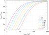 |
Fig. 1. Dependence of Ltransf/Ldisc on the transition radius, rtrans. |
The power extracted from the accretion flow evaluated in the reference frame of the corona then is
where Ltransf/Ldisc is given by Eq. (6) and ![$ U_{\!{\rm c}}^t(h,a^\ast)=[1-2h/(h^2+{a^\ast}^2)]^{-1/2} $](/articles/aa/full_html/2022/05/aa42358-21/aa42358-21-eq10.gif) accounts for the transformation of the extracted power at infinity into the local frame of corona. The subscript “c” in Eq. (8) and throughout the paper indicates quantities that are evaluated at the corona reference frame. The factor 1/2 accounts for the fact that only half of the extracted energy from the accretion flow is used to heat the corona above the accretion disc towards the direction of the observer, the other half is used for the corona on the other disc side.
accounts for the transformation of the extracted power at infinity into the local frame of corona. The subscript “c” in Eq. (8) and throughout the paper indicates quantities that are evaluated at the corona reference frame. The factor 1/2 accounts for the fact that only half of the extracted energy from the accretion flow is used to heat the corona above the accretion disc towards the direction of the observer, the other half is used for the corona on the other disc side.
2.2. X-ray energy spectrum and the size of the corona
We assumed that the X-ray corona isotropically emits (in its rest frame) a power-law photon flux of the form
where Ac is the power-law normalisation, Γ is the spectral photon index (assumed to be constant), and Ecut, c is the exponential cut-off at high energies. The X-ray spectrum extends to a low-energy rollover, E0, c. Γ and Ecut, c are free parameters of the model, while Ac and E0, c are determined by the other model parameters, as we explain below.
The value of E0, c is determined by the average energy of the seed photons, as seen by the corona,

where LBB, c and NBB, c are the luminosity and photon flux of the thermal radiation from the accretion disc illuminating the corona, both evaluated per unit area at the corona rest frame (see the following section for their estimation). The normalisation is determined as follows:
where Γf is the incomplete Gamma function, and
where L is the power given to the corona. It is either equal to Ltransf, c or, if the corona is powered by some external mechanism that is not related to the accretion process, it is a free parameter, for example Lext, c. Equation (12) states the conservation of energy: The total luminosity of the X-ray photons, LX, c, is equal to the sum of the power that is used to heat the electrons in the corona plus the energy of the photons that entered the corona and were scattered. The optical depth of the corona, τ, can be evaluated from the spectral slope Γ and the corona temperature. Γ is a free model parameter, and we assumed an electron temperature of 100 keV for the estimation of τ, like in Dovčiak & Done (2016, hereafter DD16). In the above equation, ΔSc is the local cross-section of the corona and depends on the corona radius, Rc, given in Boyer-Lindquist coordinates, as follows (DD16):
We cannot determine LX, c from Eq. (12) as ΔSc is not known. We therefore considered the fact that the Comptonisation process conserves the photon number. This implies that
where Nc is the number of the X-ray photons emerging from the corona. Equations (12) and (14) include only two unknown parameters, namely Ac (hence LX, c) and ΔSc (hence, the corona radius). Solving them eventually gives us
![$$ \begin{aligned}&R_{\rm c} = \left[\frac{L}{\pi \,(1-\mathrm{e}^{-\tau })\,U_{\!\mathrm{c}}^t\,(E_{\rm sc,c}-E_{\rm 0,c})\,N_{\rm BB, c}}\right]^{1/2}, \end{aligned} $$](/articles/aa/full_html/2022/05/aa42358-21/aa42358-21-eq18.gif)
where
is the average energy of the outgoing, scattered X-ray photons. Equations (15) and (16) are valid for both cases when L = Ltransf, c or L = Lext, c.
2.3. Thermal flux of the accretion disc received by the corona
As we showed above, the intrinsic X-ray luminosity as well as the corona radius depend on the disc thermal luminosity, LBB, c, and on the photon flux, NBB, c, evaluated at the corona rest frame. The disc spectrum at the corona is that of a multi-colour black body. The luminosity and photon number density per unit area that the corona receives from the disc when accounting for all relativistic effects is (see also Eqs. (1) and (2) in DD16)
where fcol(r) is the colour-correction factor, and Td(r) is the disc temperature (see Sect. 2.4). The integration over the whole accretion disc is done in Boyer-Lindquist coordinates. The g-factor, g(r) = Ed(r)/Ec, is the relativistic shift of the photon energy, Ed(r), when emitted from the accretion disc from radius r, to the photon energy, Ec, when received by the corona. The lensing factor, dΩc/dS(r), gives the ratio of the solid angle measured locally in the reference frame of the corona to the Boyer-Lindquist coordinate area on the disc at radius r from where photons are emitted into this solid angle, and we evaluate it numerically. The constants σ and σp are the Stefan-Boltzmann constant and its equivalent for the photon density flux.
2.4. X-ray absorption by the disc
X-rays from the corona illuminate the disc, and part of them is absorbed, acting as a second source of energy for the disc. In this case, the disc temperature, Td(r), is set by the energy released by the accretion process locally and by the X-ray absorbed flux as
![$$ \begin{aligned} T_{\rm d}(r) = f_{\rm col}(r)\,\left[\frac{F_{\rm acc}(r) + 2F_{\rm abs}(r)}{\sigma }\right]^{1/4}. \end{aligned} $$](/articles/aa/full_html/2022/05/aa42358-21/aa42358-21-eq22.gif)
 is the original black-body flux emitted by the disc, with the temperature radial profile given by NT73, and Fabs(r) is the absorbed X-ray flux. The factor 2 accounts for the fact that there are two coronæ, one on either side of the disc. We observe one of them, but the disc is illuminated and heated by both of them. Note that this is another difference with respect to K21a, who did not consider the factor of 2 in their Eq. (2). When L = Ltransf, c, then Facc(r) = 0 at r ≤ rtrans. This is because all the power dissipated to the disc below rtrans is transferred to the corona. All the energy that heats the disc at small radii is due to the X-ray absorption. On the other hand, the temperature above the transition radius is higher than in the NT73 disc because the additional absorbed flux is thermalised. Note that for L = Lext, c there is no transition region, that is, rtrans = rms.
Regarding the X-ray flux that is absorbed at each radius (due to disc illumination by the corona located on either side of the disc),

where Finc(r) and Frefl(r) are the incident and reflected fluxes, respectively. The incident energy flux, integrated in energy and evaluated per unit local area on the disc including all relativistic effects is (see e.g. Dovčiak et al. 2004, 2011)
The g−factor and dΩc/dS(r) are the same as in Eqs. (18) and (19). Like in K21a, for the total reflected flux at each radius, Frefl(r), we assumed that the local re-processing is given by the XILLVER tables (García et al. 2013, 2016), which we integrate in energy and over all emission angles. We further assumed a radially constant disc density of nH = 1015 cm−3, an iron abundance A = 1, and the high-energy cut-off value in the disc rest frame (i.e. shifted from the intrinsic value in the corona rest frame to g(r) Ecut, c).
The ionisation parameter is computed from the incident flux and the disc density. Because the XILLVER tables we used were computed assuming an X-ray spectrum with a low-energy cut-off fixed at 0.1 keV, we used only the part above g(r) E0, c (i.e. accounting for the relativistic energy shift between the corona and the disc at radius r) if g(r) E0, c > 0.1 keV. This is a small effect in the case of AGN, where the seed photon energy is far lower than in Galactic X-ray binaries, where the seed photon energy can easily be higher than 0.1 keV (see K21a for details).
2.5. Corona–disc interaction
As we explained in Sects. 2.2 and 2.3, we must know the amount of the disc thermal emission entering into the corona in order to compute its X-ray luminosity and size. At the same time, the radiation emitted by the accretion disc depends on its illumination by the corona through thermalisation of the absorbed part of the corona emission (see Sect. 2.4), hence on the X-ray luminosity and size.
To dissect this infinite loop, we used an iterative scheme in which we initially assumed that LX, c = L, that is, the second term for the incoming thermal flux in Eq. (12) is neglected. X-rays illuminate the disc, and we computed the disc illumination, Eq. (22), and the absorbed flux, Eq. (21), that determines the new disc temperature according to Eq. (20). This new temperature profile was then used to compute the incoming thermal disc luminosity and photon number density flux at the corona (Eqs. (18) and (19), respectively), and to evaluate the average seed photon energy, E0, c, and the average energy of comptonised photons, Esc, c, according to Eqs. (10) and (17), respectively. Finally, these were used to compute the new value of the X-ray luminosity, LX, c, according to Eq. (15), which was then used for the next iteration. If the neglected second term for the incoming thermal flux in the Eq. (12) contributes less than ∼20 − 30% of LX, c (which is the case for most of the parameter values relevant to AGN), the iterative scheme works relatively fast. In most cases, after the sixth iteration, the values of both LX, c and E0, c change by less than 1%, at which point the iterations stop.
The resulting radial temperature profile, Td(r), E0, c, LX, c, and NBB, c were then used to compute the radius of the corona, the final thermal flux from the accretion disc, and the primary X-ray flux (together with the disc X-ray reflection spectrum) as observed by a distant observer at infinity for a given set of the basic model parameters (i.e. MBH, ṁEdd, h, and inclination). We included all relativistic effects as detected by an observer at infinity from the accretion disc and from the X-ray source located on the system axis above the BH (see e.g. Dovčiak et al. 2004, 2011).
3. Broadband SED of the central engine in AGN
An important property of KYNSED is that it computes the broadband SED of AGN, taking into account X-ray illumination of the disc in the lamp-post geometry, assuming that the power that heats the corona is equal to the power the accretion process would dissipate to the gas below rtrans. We discuss below the effects to the SED shape of the energy transfer from the disc to the corona and of the X-ray thermalisation of the disc. We also discuss the dependence of the broadband SEDs on the main physical parameters of the model.
3.1. Effects of the energy transfer to the corona and X-ray illumination
Figure 2 shows the effects of energy transfer to the corona and of the X-ray thermalisation on the disc emission in the optical and UV bands. The dashed red lines in all panels show the SED of an NT73 disc (SEDNT) for three different spins. Relativistic effects and colour-correction factors are taken into account. The dotted blue line shows the disc SED when half of the accretion power (i.e. all the accretion power released below rtrans ∼ 5, ∼10, and ∼30 rg for a* = 0.998, 0.9, and 0, respectively) is transferred to the X-ray corona and the X-rays do not illuminate the disc, that is, without thermalisation. In this case, both Facc(r) and Fabs(r) in Eq. (20) are zero at r < rtrans. Consequently, the disc does not emit below rtrans, most of the far-UV emission is missing, and the whole SED is shifted to lower energies. At radii larger than rtrans, the disc emits as an NT73 disc, the disc temperature is the same in both cases, hence both the dashed and dotted SEDs are identical above a certain wavelength.
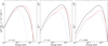 |
Fig. 2. NT disc spectra (dashed red lines) and KYNSED disc SEDs with and without thermalisation (solid black lines and dotted blue lines, respectively) for a* = 0, 0.9 and 0.998 (left, middle, and right panel, respectively). The physical parameters are MBH = 5 × 10⁷ M⊙, Ltransf/Ldisc = 0.5, ṁEdd = 0.1, θ = 40°, h = 10 rg, Γ = 2, and Ecut, obs = 300 keV. |
The solid black lines show the KYNSED SED when X-ray thermalisation takes place. The disc temperature at radii larger than rtrans is higher than the NT73 temperature in this case. As a result, X-ray illuminated discs emit more than the NT73 disc at lower energies (i.e. at longer wavelengths that are produced mainly at larger radii). The effect is more pronounced in the case of high spins because the intrinsic NT73 temperature is lower in these discs at large radii: due to enhanced efficiency, the accretion rate in physical units decreases (for the same accretion rate in Eddington units), and so does the original NT73 disc temperature. Therefore, for the same amount of transferred energy, Ltransf, the effects of X-ray thermalisation increase with increasing spin (see also K21a) and are visible up to higher energies (because rtrans is smaller).
At the same time, the disc below rtrans is no longer cold. The disc emits all the way down to rISCO because it absorbs the incident X-rays. This effect is much more pronounced for slow BH spin, where the transition radius rtrans is much larger for the same amount of the transferred energy, Ltransf.
The overall SED clearly approaches SEDNT for slow spin because the temperatures in the large region below rtrans (rtrans ∼ 30 rg for the spin a* = 0) are just redistributed; the transferred energy, Ltransf, that is used for the illumination, absorption, and eventually for the thermalisation mainly in this inner region, compensate for the original missing NT73 disc emission. However, for fast spins, the transferred energy, Ltransf, is extracted from a much smaller region (rtrans ∼ 3 rg for the spin a* = 0.998) while it illuminates larger region, which means that it increases the temperatures of the original NT73 disc above rtrans (compare the black and red lines in all panels of Fig. 2). This behaviour depends on the height of the corona and on the amount of the extracted energy (and thus on the size of rtrans).
3.2. Effects of the model parameters on the SED shape
Figures A.1–A.3 in the appendix show the broadband KYNSED SEDs for various spins, BH masses, and accretion rates. In general, the disc temperature increases with increasing spin, decreasing BH mass, and increasing accretion rate, as expected. The sharp flux increase at the far-UV that appears in many SEDs indicates the low-energy cut-off of the X-ray spectrum, E0. At energies above E0, the disc SED is enhanced due to the contribution from the X-ray continuum. For the model parameters we have assumed, the model predicts E0 values of ∼0.01 keV (i.e. ∼1250 Å) when MBH = 109 M⊙ (see the upper SEDs in Fig. A.2) and when ṁEdd ≤ 0.1 (see the respective SED in Fig. A.3). The seed photon energy, E0, increases and the flux jump is more pronounced for fast spins because of the higher disc temperature in the inner accretion disc. Because of higher E0 and the same extracted energy, Ltransf, the normalisation of the primary X-ray flux, Ac, is higher. The flux increase could be observed in the far-UV spectra for the right combination of parameters, but it will not be easily visible. Most of the time, the flux jump is of a low amplitude, and in any case, the flux increase should be smoother than shown in these plots. In reality, we do not expect the low-energy cut-off in the X-ray spectrum to be so sharp.
We kept Ltransf/Ldisc, Γ, and the high-energy cut-off constant in Figs. A.1–A.3. The normalisation of the X-ray spectrum changes because the total available energy increases with increasing BH mass and accretion rate, but the shape of the X-ray spectrum remains roughly the same. However, at low energies, a significant excess emission on top of the power-law continuum below 1 − 2 keV is evident in some SEDs. See for example the SEDs when MBH ≤ 5 × 10⁷ for spins a* ≥ 0.9, and when MBH ≤ 107 M⊙ for all spins (Fig. A.2). This excess flux in these cases is mainly due to the thermal emission of the disc.
Figure A.4 shows the AGN SEDs for various Ltransf/Ldisc values. As expected, the X-ray spectrum normalisation increases in proportion to Ltransf/Ldisc. However, although the fraction of the accretion power transferred to the corona increases, the optical and UV SED does not decrease accordingly. In fact, the optical and UV emission below ∼0.05 keV increases with increasing Ltransf/Ldisc (this is clearly visible in the high-spin SEDs). This is due to the assumption of isotropic X-ray emission (in the corona rest frame), which implies that at least 50% of the emitted X-ray luminosity returns to the disc (more, if the corona height is less than 10 rg), becomes absorbed, and increases the disc emission. Even when Ltransf/Ldisc = 0.9, the optical and UV peak is still larger than the SED peak in the X-rays. Moreover, two-component thermal emission may be present for very high Ltransf/Ldisc, especially in the low-spin case (see the left panel of Fig. A.4); the two components correspond to the two regions above and below the rtrans. The transition radius is quite large in this case (e.g. rtrans ∼ 200 rg for spin a* = 0 and Ltransf/Ldisc = 0.9; see Fig. 1), and the thermal radiation in these two regions may have quite different peak temperatures (especially for low heights when the illumination is concentrated in the region close to the BH).
The corona height affects the full-band SED significantly. The observed X-ray luminosity decreases significantly when h ≤ 10 rg (see Fig. A.5) even though Ltransf/Ldisc remains constant. This is due to light-bending: most of the X-rays fall into the BH or illuminate the inner disc when the corona is close to the BH. As the corona height increases, the absorbed X-ray flux at larger radii increases because of an increase in the photon incident angle (see also K21a). As a result, the disc temperature at larger radii increases in response to the corona height, and so does the flux at longer wavelengths (i.e. below ∼0.01 keV) for all spins. The opposite effect is observed at higher energies. The photon incident angle in the inner disc does not vary significantly with the height of the corona. However, as the height increases, the incident X-ray flux on the inner disc decreases, and so does the disc temperature, below rtrans. Consequently, the disc emission above 0.01 keV decreases with increasing height. This is more prominent for high spins.
The inclination angle strongly affects the disc emission (and the X-ray reflection spectrum) but not the X-ray continuum because we have assumed that the corona emission is isotropic in its rest frame. At high inclinations (θ ≥ 70°), the disc flux is substantially decreased (see Fig. A.6). The flux jump at ∼0.03 − 0.05 keV is most evident in this case. If the molecular torus does not block the view to the central nucleus in luminous AGN, this feature should be observed in the far-UV spectra of highly inclined sources at redshifts higher than ≥3 (for the parameters chosen in Fig. A.6).
Figures A.7 and A.8 show the effects of Γ and Ecut in the SED. A softer spectrum results in a stronger soft-excess (around 0.3–1 keV) and in a stronger flux jump at E0 (Fig. A.7). The X-ray spectrum normalisation at 1 keV decreases with increasing Ecut (Fig. A.8) even though Ltransf/Ldisc remains constant. This is because when rtrans is determined, both Ltransf/Ldisc and E0 are fixed (for a given combination of MBH, ṁEdd, a*, and h). Therefore, the X-ray spectrum normalisation is uniquely determined from the photon index, Γ, and Ecut. For the same Γ, the normalisation decreases as Ecut increases, and the (fixed) X-ray luminosity is spread over a larger energy band.
3.3. Comparison with AGNSED
Figure 3 shows a comparison between KYNSED and AGNSED for an AGN with MBH = 5 × 10⁷ M⊙ and ṁEdd = 0.1, for a* = 0, 0.9, 0.998. The dotted black line shows the KYNSED SED when fcol = 1 (which is what AGNSED assumes), and the solid black line shows the KYNSED model when we adopt the Done et al. (2012) prescription.
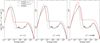 |
Fig. 3. Comparison between KYNSED and AGNSED (red) for a* = 0, 0.9, and 0.998 (left to right). The inclination is 40 degrees and Γ = 2 in both models. The dotted and solid black lines show the KYNSED model without the spectral hardening effect (colour-correction factor fcol = 1) and when the spectral hardening is computed following the Done et al. (2012) prescription (fcol = −1), respectively. |
To the best of our knowledge, AGNSED is the only other model for the broadband AGN SEDs (like KYNSED). The accretion flow in AGNSED is assumed to be radially stratified. It emits as a standard (i.e., NT73) disc black body from the outer disc radius to Rwarm, and in the region between Rwarm and a smaller radius, called Rhot, the model assumes the passive disc scenario of Petrucci et al. (2018). This is the so-called warm Comptonisation region, which is thought to be responsible for the observed soft X-ray excess in AGN. At a radius smaller than Rhot, the disc is truncated. Like KYNSED, AGNSED assumes that the accretion power that would be dissipated in the disc below Rhot is transferred to the hot Comptonisation component, which is responsible for the X-ray continuum in AGN.
We have assumed Ltransf/Ldisc = 0.5 in KYNSED for the spectra shown in Fig. 3. We also set Rhot = 31.55, 10.96, and 4.77 rg for the AGNSED spectra shown in the same figure for a* = 0, 0.9, and 0.998, respectively, so that the energy transferred to the hot Comptonisation component was equal to half the total accretion power. We set the corona height at 10 rg and Ecut at 300 keV in KYNSED. For AGNSED, we did not consider the warm corona, and we set kTe = 150 keV.
An obvious difference between the two models is the presence of the X-ray reflection features in KYNSED. This is because AGNSED does not consider X-ray reflection from the disc. There is a large difference between the X-ray continuum normalisation in KYNSED and AGNSED. To a large extent, this must be due to the fact that the corona in KYNSED emits isotropically to all directions, so that half of the X-ray power is directed away from the observer to the disc (which extends to rISCO and blocks emission from the corona, which is located on the other side of the disc). On the other hand, there is no disc (physically) below Rhot in AGNSED, hence the observer can detect emission from the whole of the corona. The KYNSED and AGNSED SEDs show differences in the optical and UV bands as well at all spins. There are significant differences even when we adopt fcol = 1. In the a* = 0 case, the difference in the far-UV is probably due to the X-ray heating of the inner disc (below rtrans) in KYNSED. The disc in AGNSED does not exist below Rhot, while the disc extends down to rISCO in KYNSED. Although the power that is dissipated due to the accretion process below rtrans is transferred to the corona, the disc is illuminated by the X-rays. Most of them are absorbed, and the disc is heated. As a result, the disc emits, mainly in the UV, hence the difference with AGNSED in these wavelengths.
At higher spins, the AGNSED optical and UV flux increases and in fact overcomes the KYNSED flux (below ∼0.01 keV) when a* = 0.998, although the disc in KYNSED emits down to rISCO, while the disc is truncated at Rhot in AGNSED (below which half of the disc power is emitted). This discrepancy is probably due to the fact that AGNSED does not take general relativistic (GR) effects into account. Due to GR effects, a large amount of flux from the inner disc will end up in the BH and the disc, hence the difference in the two spectra.
The comparison between the solid and dotted black lines in Fig. 3 shows that the choice of fcol significantly affects the optical and UV spectrum. For the adopted model parameter values, the Done et al. (2012) prescription significantly alters the spectrum in the optical and UV band. The choice of fcol affects the X-ray spectrum as well, as E0 depends on the disc temperature (although the differences between the solid and dotted lines in the X-ray band are not that significant).
We have assumed Ltransf/Ldisc = 0.5 for the KYNSED spectra in Fig. 3. This implies that the same amount of power that is released as the disc thermal radiation is also transferred to the corona. This power is used to heat the electrons, and then it is assumed to be released in its entirety as X-ray luminosity (see Eq. (12), which shows that the X-ray luminosity is equal to the total power transferred to the corona plus the luminosity of the soft photons that are scattered in the corona). However, as the left panel of the figure shows, the total X-ray flux appears to be far lower than the total thermal flux.
One reason for this is that the thermal energy is emitted as the cosine source (i.e. as μ L/π; here, μ = cos θ is the cosine of the inclination angle, and L is the power given to the disc and to the corona, which are assumed to be equal), while the X-ray source is assumed to be isotropic (i.e. L/4π). A second reason is that half of the X-ray emission is incident to the disc, where most is absorbed (for a neutral disc, it can be as high as 80%) and the rest is reflected in X-rays (the other 20%). Thus, the total thermal radiation should be μ L (1 + 0.8/2)/π, while the total X-ray emission is L/4π + μ 0.2 L/2/π. This approximate estimate predicts a ratio of the observed X-ray emission and the disc thermal radiation of 30% (for an inclination of 40°). A precise measurement shows that the total observed X-ray flux makes up only 22% of the total observed thermal flux in the KYNSED spectra shown in the left panel of Fig. 3. The difference with the result from the approximate computation arises because in the latter case we exclude all the nuances of the computations, including the radial dependence of the emission and illumination and relativistic effects.
4. Fitting the average broadband spectrum of NGC 5548
As an example of how KYNSED works in practice, we chose to fit the average SED of NGC 5548. This is a typical Seyfert 1 galaxy, at a distance of DL = 80.1 Mpc according to NED1. It has been observed extensively in the past at all wavebands. In particular, NGC 5548 was observed by Swift, the HST, and many ground-based optical telescopes from February to July 2014. These observations were part of the Space Telescope and Optical Reverberation Mapping project (STORM; De Rosa et al. 2015). Swift observed the source over 125 days with a mean sampling rate of ∼0.5 day in X-rays and across six UV and optical bands. Approximately daily HST UV observations were also obtained. The ground-based optical monitoring observations resulted in light curves with a nearly daily cadence in nine filters, namely B, V, R, I and u, g, r, i, z (see e.g. Edelson et al. 2015; Fausnaugh et al. 2016). These observations resulted in X-ray, UV and optical light curves that are among the densest and most extended light curves ever obtained for an AGN. Edelson et al. (2015) and Fausnaugh et al. (2016) used these light curves to compute the X-ray to UV and optical time-lags, and K21b fitted them using the K21a model. Therefore, it is interesting to fit the average SED of NGC 5548 using the same data set that K21b used to fit the optical and UV time-lags, and investigate whether the same model can fit both the average SED and the X-ray, optical and UV time-lags with the same best-fit parameters. K21b fitted the time-lags of other AGN as well, but we chose NGC 5548 because the host galaxy contribution in the optical and UV bands is quite well known for this object (see Mehdipour et al. 2015; Fausnaugh et al. 2016).
4.1. Average SED
We used the data from the 2014 multiwavelength campaign to compute the mean SED of NGC 5548. Regarding the UV and optical band, we used the data in Fausnaugh et al. (2016). These authors computed the mean of all light curves in 18 spectral bands (from ∼1160 − 9160 Å) and list the results in Col. 8 of their Table 5. Mean fluxes are corrected for Galactic extinction, and their error is equal to the rms scatter of the points in the light curve. Fausnaugh et al. (2016) also list the host galaxy contribution in each band, which we subtracted from the mean observed flux.
As for the X-rays, first we considered the 2 − 10 keV Swift/XRT light curve, and we realised that the count rate in the time interval between 56712 − 56714 MJD, 56775 − 56785 MJD, and 56807 − 56812 MJD is close to the overall mean count rate. There are 5, 20, and 14 observations during these intervals, respectively. We used data from all the observations in each interval, and we extracted the overall X-ray spectrum of each interval using the automatic Swift/XRT data product generator2 (Evans et al. 2009). We considered the 0.4 − 8 keV band in each spectrum, and grouped the spectra to have at least 25 counts per bin.
The flux measurements from broadband UV and optical filters can be affected by emission from the Balmer continuum, blended Fe II, and other emission lines that originate in the broad-line region (BLR; e.g. Korista & Goad 2001, 2019). Fausnaugh et al. (2016) estimated that the Balmer continuum emission accounts for about 19% of the flux in the u and U filters, and the Hα line contributes ∼20 and 15% of the flux in the r and R bands, respectively. We therefore excluded these points when we fitted the data. We also excluded the Swift/UVOT M2 and W1 data (in the 2000 − 3000 Å range), as they may also be affected by the Balmer continuum emission.
4.2. Theoretical model
We fitted the three X-ray spectra and the UV and optical data simultaneously. The spectral fitting was performed using XSPEC (Arnaud 1996). We used the FTOOLS command ftflx2xsp3 to create spectral files in the UV and optical range in a format that is compatible with XSPEC. The overall model, written in XSPEC parlance, is as follows:
We used KYNSED twice; once for the optical and UV and then for the X-ray spectra. Obviously, all the relevant KYNSED parameters were tied in the UV and optical range with those in the X-ray range. The TBabs component (Wilms et al. 2000) accounts for the effects of the Galactic absorption in the X-ray band (the UV and optical data points are already corrected for Galactic extinction). We fixed its column density to 1.55 × 1020 cm−2 (HI4PI Collaboration 2016). All model parameters were tied together in the X-ray spectra, as they are all considered to be representative of the mean X-ray spectrum, that is, they are treated as data sets of the same intrinsic spectrum.
4.3. Host galaxy absorption
We also considered the possibility of intrinsic absorption in the host galaxy. We considered the extinction curve of Czerny et al. (2004) for the absorption in the optical and UV bands. The extinctionCzerny component is determined by E(B − V)host, which we left free during the model fitting. The zTBabs component accounts for the absorption in the X-ray band of the same absorber, and its column density was kept linked to E(B − V)host through the relation NH, host = 5.8 × 10²¹E(B − V)host cm−2 (Bohlin et al. 1978). Finally, we used the spectral component zxipcf (Reeves et al. 2008) to account for possible warm absorption. This component accounts for absorption from partially ionised absorbing material, which covers some fraction of the source, while the remainder of the spectrum is seen directly. We left all the parameters of this component free during the model fitting.
4.4. Fitting process
We chose to fit the data by assuming that the X-ray source is powered by the accretion process. In addition to rtrans, the other KYNSED physical parameters in this case are black-hole mass and spin, Ltransf/Ldisc, accretion rate, corona height, photon index, high-energy cut-off, and inclination. We fixed the BH mass at 5.2 × 10⁷ M⊙ (Bentz & Katz 2015), and we assumed a high-energy cut-off of 150 keV (Ursini et al. 2015). Still, there are too many parameters to constrain by fitting the data. For example, the figures in the appendix show that spin, accretion rate, and inclination affect the optical and UV SED significantly. The corona height also affects the optical and UV, as well as the X-ray normalisation, together with Ltransf/Ldisc and Γ. We therefore decided to fit the data by considering a grid of height values from h = 2.5 rg to h = 10 rg, with a step of 2.5 rg, and from 10 to 80 rg with a step of 5 rg. At each height, we left the spin, inclination, photon index, Ltransf/Ldisc, and ṁEdd free to vary.
4.5. Best-fit results
The model fits the data very well at all heights, with pnull > 0.1. This is probably due to the effect we mentioned in the previous subsection: many model parameters affect the shape of the SED. As height changes, other physical parameters such as ṁEdd, Ltransf/Ldisc, and inclination also change in a way that the final fit is always acceptable. The best-fit values of each of the parameters are shown as a function of height in Fig. 5. The plots show that the spin varies from ∼0.8 − 1, Ltransf/Ldisc from ∼0.4 − 0.7, and ṁEdd from ∼0.05 to 0.15 (a difference of a factor of 3) as we increase the height from ∼5 to 85 rg.
The best-fit parameters for all absorption components do not depend on the corona height (therefore we do not plot them in Fig. A.5). We found E(B−V)host = 0.12 ± 0.02 mag for the host galaxy extinction (all errors are 1σ errors unless otherwise stated). This is consistent with the E(B − V) value of  that Panagiotou et al. (2020) reported from modelling the optical and UV PSDs (which were estimated using light curves from the 2014 monitoring campaign as well). Kraemer et al. (1998) reported a reddening of
  of the narrow-line region in NGC 5548. The portion of the reddening that is due to our own Galaxy is small (Schlafly & Finkbeiner 2011, ∼0.016), therefore this value is also consistent with our measurement. In addition, in our modelling, the absorber in the optical and UV band is linked to absorption by neutral gas in the X-ray band. The best-fit E(B − V) value implies a neutral absorber with NH ∼ 6 × 1020 cm−2. This is almost identical to the NH measurement of Mathur et al. (2017) when they fit Chandra spectra taken during the STORM campaign, with a power law plus a warm corona model. As for the ionised absorber, we found that NH ∼ 2 × 1022 cm−2, log(ξ/erg cm s−1) ∼ 1, and fcov = 0.94 − 1.
The fit results in a high spin value of a* > 0.8 for all heights (see the top panel in Fig. 5). This is in agreement with the results obtained by K21b, who found that the a* = 1 case was preferred because the resulting accretion rate was consistent with the value of ṁEdd = 0.05 that is reported in the literature for NGC 5548.
As we have already discussed in Sect. 2.2, KYNSED also computes Rc, assuming conservation of the photon number during Comptonisation. This model parameter is not used to fit the data, but it is computed when model fitting is completed, and can be viewed using the XSPEC command xset. The corona radius can be used to check the physical consistency of the model because Rc should be smaller than the height of the X-ray source minus the event horizon radius, RH. The dashed black line in panel f of Fig. 5 shows (h − RH) as a function of h. Below h = 7.5 rg, (h − RH) is always smaller than Rc. Clearly, despite the low χ2 values, we reject all heights smaller than h = 7.5 rg as physically unacceptable solutions.
We can use the results from the K21b fits to the time-lag spectra of NGC 5548 to place additional constraints on the coronal height range that would be acceptable from a physical point of view. We therefore considered the 1σ confidence region for height from fitting the time-lag spectrum in K21b (33 − 77 rg for a* = 1) to constrain the best-fit results to the mean SED even further. The respective 1σ confidence region on the height is indicated by the grey shaded area in Fig. 5. The solid vertical line in Fig. 5 indicates the best-fit height we obtained in K21b (h = 46 rg). The fit to the energy spectrum in this range is statistically acceptable and predicts a very high spin value (a* > 0.94). This result indicates how powerful it is to combine spectral and timing information to constrain the model. K21b could fit the time-lags equally well, both when assuming a* = 0 or 1. When combined with the fitting of the SED, the hypothesis of a* = 0 is no longer accepted.
Table 1 lists the range of the best-fit model parameter values that correspond to heights in the 33 − 77 rg interval. The transition radius range of ∼5 − 10 rg implies a rather small disc region, close to ISCO, where accretion power is transferred to the corona. However, because the best-fit BH spin is high, this power is large (at least ∼50% of the total disc luminosity is transferred to the corona).
The best-fit accretion rate range is fully consistent with the ∼5% value, which is based on bolometric luminosity estimates (Fausnaugh et al. 2016). It is also consistent with the accretion rate estimates from the fitting of the time-lag spectra. K21b found ṁEdd = 0.03, with a 1σ confidence region of [0.005–0.05] (see their Table 3). Our 1σ confidence region almost overlaps with theirs, indicating the agreement between the two approaches (within 1σ). We note that K21b assumed Γ = 1.5, based on the results of Mathur et al. (2017). This is different from our best-fit results of Γ ∼ 1.75, but the time-lags do not depend on Γ as long as Γ ≤ 2 (see Fig. 19 in K21a). Therefore, the K21b model would fit the NGC 5548 time-lags equally well even if they had assumed a photon index of 1.7–1.8. Our best-fit results of ∼50° −70° for the disc inclination is rather large for a type 1 AGN. Interestingly, Pancoast et al. (2014) found that the geometry of the Hβ BLR in NGC 5548 is that of a narrow thick disc (see Fig. 1 in their paper) with an inclination angle of 38.8 degrees. This agrees (within 1σ) with our results, which implies that the inclination of the BLR disc and the accretion disc may be similar in NGC5448, and that it may be slightly higher than the 40 degrees that are typically assumed for type I AGN.
As described in the KYNSED model documentation, the XSPEC command xset outputs various computed values of the system properties such as the value of the ionisation parameter at the inner and outer edge of the accretion disc, the intrinsic and observed X-ray luminosity of the primary X-ray source in the 2–10 keV energy band, the reflection ratio, the ISCO and transition radius, as well as the optical depth and the electron density in the corona. For a height 46 rg (indicated by the vertical black line in Fig. 5), we obtain the best-fit to the model for a = 0.998, θ = 55.9°, Γ = 1.756, Ltransf/Ldisc = 0.68, and ṁEdd = 0.052 (see Fig. 5). Then, the command xset lists the corona radius, Rc = 15.3 rg, optical depth, τ = 1.2, electron column density, Σe = τ/σT = 1.8 × 1024 cm−2 (where σT = 6.652 × 10⁻²⁵ cm2 is Thomson cross-section), and the electron density in the local frame of the corona,  .
.
Figure 4 shows the mean optical, UV and X-ray SED of NGC 5548, constructed as we explained above. The solid and the dashed lines in the same figure correspond to the absorbed and unabsorbed best-fit model, respectively, when h = 46 rg. The dot-dashed lines in the same figure show the individual spectral components of the best-fit model to the broadband SED, that is, the disc thermal emission (including thermalisation due to the absorbed X-rays), the X-ray emission from the corona, and the X-ray reflection component (both the overall and the individual spectral components are plotted as seen by a distant observer). The model fits the data well (χ2 = 415.6/388 d.o.f.). Open symbols in Fig. 4 show the M2, W1, U, u, R, and r -band measurements that we did not consider during the model fitting. The observed average flux in these bands is indeed higher than in the best-fit model. We estimate this excess to be ∼10 − 30% in the M2 to U bands and ∼20 − 40% in the r and R bands, respectively. These values are consistent with those estimated by Fausnaugh et al. (2016) as the contribution of the BLR to the observed flux in the same bands.
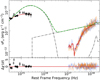 |
Fig. 4. Observed broadband NGC 5548 SED. The solid red line shows the model obtained for h = 46 rg. The dashed green line shows the unabsorbed best-fit model (i.e. by removing all Galactic and intrinsic neutral and warm absorbers). The dash-dotted black lines show the various spectral components. Empty circles indicate the data points that we did not consider during fitting, to avoid contamination from the BLR (see Sect. 4 for details). The grey, blue, and orange data points indicate the three X-ray spectra we used in the fitting. |
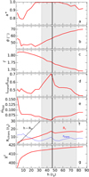 |
Fig. 5. Best-fit parameters obtained by fitting the NGC 5548 broadband spectra for various corona heights. The vertical solid line and the grey shaded area indicate the best-fit value and the 1σ confidence range, respectively, of the height obtained by fitting the time-lag spectrum of this source with a* = 1 in K21b. The dashed black line in panel f shows the difference between the corona height and the event horizon, and the dotted blue line in the same panel shows the best-fit rtrans that corresponds to the fitted values of transferred energy, Ltransf/Ldisc, and black-hole spin, a*. |
5. Discussion and conclusions
We presented a new model for the broadband SED of AGN from optical to X-rays. The model includes an X-ray illuminated standard NT73 disc, where all the relativistic effects are taken into account. We also include a colour-correction factor, following the prescription of Done et al. (2012). The model assumes that the X-ray corona is located at height h above the BH (the lamp-post geometry) and emits isotropically in its rest-frame. We took all the relativistic effects into account when we calculated the photon path from the disc to the corona and back, and when we calculated the path from the disc and the corona to the observer at infinity.
The KYNSED model can be used in the XSPEC spectral fitting package. It is publicly available, and it can be downloaded from https://projects.asu.cas.cz/dovciak/kynsed. A file called KYNSED-param.txt describes all the model parameters and can be downloaded from the same web address.
5.1. X-ray luminosity
The power that is given to the corona can either be a free parameter or it can be linked to the accretion power. In the second case, the model assumes that the total accretion power that is dissipated below a transition radius, rtrans, is transferred to the X-ray corona. The mechanism that feeds the corona may not be 100% efficient, and the power that is transferred to the hot corona may not be exactly equal to Ltransf, as defined by Eq. (4). The fraction of the power that is dissipated to the disc when the cold matter accretes over the power that is transported to the corona could be an additional free parameter of the model, but this is not currently incorporated in the model. In its current version, the model with a particular transition radius, rtrans, gives an upper limit of the X-ray normalisation.
It is also possible that the corona is powered by another source of energy, for example by the Blandford-Znajek process (Blandford & Znajek 1977). This mechanism is assumed to power the jets in radio-loud AGN. This possibility can be accommodated in our model if rtrans is set equal to rms. In this case, the energy that is provided to the corona, Lext, is a free model parameter. The only difference then is that the disc emits, like an NT disc, down to rISCO, and it is also heated by the X-rays, which take the power from somewhere else.
5.2. Low-energy X-ray cut-off
We took all transformations to the photons energy (due to GR effects) from the disc to and from the corona rest-frames and to the observer into account. In particular, KYNSED self-consistently computes the low-energy cut-off in the X-ray spectrum, E0, using an iterative process that takes the average energy of the disc photons that arrive at the corona (in its rest frame) into account. This depends on the accretion rate and rtrans, but also on the X-ray flux illuminating the disc (which, in turn, depends on E0).
The correct estimation of E0 is important for two reasons. On the one hand, if the spectral slope and the high-energy cut-off can be determined by the X-ray data, then the X-ray normalisation is uniquely determined as long as E0 is set. This may have important implications for the determination of the X-ray continuum amplitude and the study of the iron-line shape in the X-ray spectra of AGN. Secondly, E0 is necessary for the accurate calculation of the incident, reflected, and absorbed X-ray flux on each disc element above and below rtrans and hence for the determination of the disc heating and its temperature.
5.3. Corona height and size
KYNSED may overestimate the corona height. The model assumes a flat disc, which disagrees with the standard SS73 and NT73 predictions. Although low, the ratio of disc height to radius in these models is not zero. We expect the disc height to increase with increasing radius. Even a small increase of the disc height will affect the incident angle of the X-ray photons arriving on the disc surface. This will increase the incident and the absorbed X-ray flux in each disc element. It is therefore possible that coronæ with smaller heights will be able to heat the disc more efficiently, and perhaps fit the data with the same quality when the height is larger. We plan to update KYNSED with an advanced treatment of the X-ray illumination of discs with non-zero height in the future.
The model computes the X-ray corona size using the conservation of photons during the Comptonisation process. This computation is approximate because it assumes a fixed corona temperature and an approximate relation between the optical depth of the corona and its temperature (see Sect. 2.2). Nevertheless, an inspection of the size of the corona after fitting the data can provide useful constraints on the validity of the model. If the radius is considerably larger than its height (e.g. by a factor of ∼2 or more), this would indicate that the adopted lamp-post geometry is not consistent with the observed SED (see also Ursini et al. 2020, where the estimation of the size of the corona from 3D computations is discussed).
To confirm the validity of the point-source approximation, we computed the Comptonised spectra emerging from the corona with realistic (non-infinitesimal) size with the 3D Monte Carlo code MONK, see Zhang et al. (2019), which includes all relativistic effects. We considered three heights of the X-ray corona, h = 3, 10, and 30 rg, and we considered several sizes, from a small to a very large corona that would even reach as far as the BH horizon. The corona was assumed to be static and homogeneous with an optical depth that would result in a power-law-like energy spectrum with an index Γ ≈ 2. The electron temperature was set to Te = 100 keV. Because the MONK code does not yet include corona–disc interaction and thermalisation of the illumination in the accretion disc, we assumed the NT73 radial temperature profile, TNT(r), and we set the inner disc edge at ISCO. Furthermore, we assumed a BH mass MBH = 5 × 10⁷ M⊙, a BH spin a = 1, an accretion rate ṁEdd = 0.1, an inclination θ = 40°, and we set the temperature hardening factor to fcol = 1.
The colour lines in Fig. 6 show the MONK results. The spectra plotted in this figure show the luminosity divided by  so that we will be able to compare them directly with the KYNSED results, as we discuss below. The resulting Comptonised emission per
  gives a slightly higher normalisation for larger sizes. This is more pronounced when the corona is located farther away from the BH.
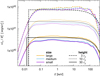 |
Fig. 6. Comparison of the primary X-ray spectra in the point source approximation used in KYNSED (black lines) with the 3D corona Monte Carlo computations of MONK (colour lines) for the spherical corona with different sizes, small (magenta), medium (blue), and large (yellow), at three heights. The three radii of the corona are Rc = 0.5, 1.5, and 2 rg for the height h = 3 rg; Rc = 1, 6, and 9 rg for the height h = 10 rg; and Rc = 5, 15, and 29 rg for the height h = 30 rg. The corona with the largest size extends as far as the BH horizon. The luminosities are divided by |

We used the same set-up as in KYNSED assuming an accretion disc with TNT(r) radial temperature profile, starting at ISCO, and without thermalisation due to the disc illumination. To achieve this, we used the model option with an external energy source, Lext. Regarding the high-energy cut-off in KYNSED, we assumed its value to be Ecut = 250 keV because it is thought to be approximately 2–3 times higher than the electron temperature, see for example Petrucci et al. (2001). The low-energy cut-off, E0, was computed as an average energy of the thermal disc photons illuminating the corona, as we described above, see for instance Eq. (10). Furthermore, in order to properly compare the normalisation of the KYNSED with the MONK spectra, we chose Lext to have the right value at each height so that the resulting size of the corona Rc was 1 rg. In this way, the resulting KYNSED spectrum is identical to the spectrum in units of power per unit area, and it can directly be compared with the MONK spectra, normalised to unit area. For this comparison, the external energy feeding the corona, Lext, decreases with the height in the KYNSED model for the constant Rc = 1 rg, therefore the normalisation of the primary X-ray spectra in Fig. 6 decreases with height as opposed to Fig. A.5, where the energy transferred to the corona, Ltransf/Ldisc, was kept constant.
The KYNSED spectra are depicted in Fig. 6 by the solid black line. Figure 6 shows that the MONK and KYNSED spectra are quite similar. The KYNSED low-energy cut-off corresponds quite well to the energy at which the Comptonised emission in the MONK spectra starts to decrease. The same is true for the high-energy cut-off in the MONK and KYNSED spectra. It is perhaps even more interesting that the normalisation of the KYNSED spectrum is always very close to the MONK spectra. The maximum difference between the KYNSED normalisation and the MONK spectra is a factor of 1.45. This would correspond to a relative error on the corona radius of about 20% ( ).
).
To conclude, our results indicate that the point-source approximation used in KYNSED approximates the spectrum of a 3D corona very well. The similarity between the MONK and KYNSED spectra suggests that the X-ray spectrum detected by the distant observer and the X-ray spectrum illuminating each disc element are the correct spectra even if the emission originates from a 3D corona, with a radius like the one that KYNSED computes at the end of the data fitting. This statement holds if the disc illumination of a point-like and a 3D corona are also similar.
Regarding the effects of the size of the corona with respect to the disc illumination, some extended geometries have already been studied in the past. For example, Dauser et al. (2013) studied the disc illumination by a vertically extended corona. They find that, in general, the incident radiation on the disc as a function of radius does not differ significantly from that of a point-like source located close to the centre of the jet-like structure. See for example the dashed green and solid red line in the left panel of their Fig. 7. There are differences, but the overall shape of the irradiation flux profile remains roughly similar. Dauser et al. (2013) only tested the vertical extension of the corona, which is different from the 3D geometry of a spherical source. However, Zhang et al. (in prep.) studied the disc irradiation in the case of a 3D spherical corona when the BH spin axis is an axis of symmetry. They found that the disc illumination pattern of the 3D corona and of a point-like source located in its centre are quite similar, for instance for the corona at height 10 rg the illumination profile is practically identical for the corona with its radius up to 4 rg. For reasonable sizes of the corona, the illumination pattern is therefore not expected to differ much from the point-like approximation.
5.4. Accretion disc density, ionisation, and accretion rate.
In the KYNSED model, the X-ray reflection as well as the partial absorption of the disc illumination by the corona is computed from disc reprocessing tables. As stated earlier, we used the XILLVER tables by García et al. (2013, 2016). These tables have two different flavours. In the first table, the high-energy cut-off is one of the free input parameters while the disc density is kept constant, and in the second option, the disc density is a free input parameter while the high-energy cut-off is kept at a constant value. Thus, unfortunately, we cannot change both the density and Ecut with radius in our model.
The high-energy cut-off of the incident spectrum on each disc element is shifted due to relativistic effects, therefore the reflection and thus also the absorption changes with radius. Furthermore, the normalisation of the Comptonised X-ray spectrum depends on the high-energy cut-off; see for example Fig. A.8 in the appendix. KYNSED therefore operates with the assumption of a constant disc density.
X-ray absorption by the disc will depend on the disc ionisation (a more ionised disc reflects more, thus absorbs less), and the ionisation will depend on the disc density, which decreases with radius farther out from the centre. The ionisation also depends on the illumination, which decreases with radius faster then density. We expect most of the outer parts of the disc to be neutral, and thus the absorption will not change much with radius due to changing ionisation. Only the very inner parts of the accretion disc will be affected.
It is possible that standard accretion discs are thermally stable until the accretion rate becomes ∼0.3 of the Eddington limit (e.g. Yuan & Narayan 2014, and references therein). In this case, results may not be reliable when broadband SEDs of AGN are fit with high accretion rates with any disc model. However, this may not be true for disc models like KYNSED when a large amount of power is transferred from the disc to the corona. Svensson & Zdziarski (1994) investigated the case when a major fraction, f, of the power released during the accretion process is transported to and dissipated in the corona. They showed that this has major effects on the cold disc, making it colder, more geometrically thin, denser, and with larger optical depths. One important consequence is the disappearance of the effectively optically thin zone as well as of the zone dominated by radiation pressure for f values close to unity (as in our case). Svensson & Zdziarski (1994) studied the case when f remains constant at all radii, while f = 1 below rtrans and 0 at larger radii in KYNSED. However, the zone dominated by radiation pressure is typically located in the inner disc. Hence the KYNSED set-up may result in disc solutions in which gas pressure dominates at all radii, and the disc may be stable against thermal and viscous instabilities at higher accretion rates. Although these authors only studied the case of spin zero, similar results may hold for higher spins as well. This may in effect cause that if the corona is fed by the accretion flow itself, the geometrically thin accretion disc may exist even for higher accretion rate values than the typically assumed upper limit of about 0.3.
5.5. Fitting SEDs in practice
KYNSED does not take variability into account in its computations. It assumes that the spectral properties do not change in the timescale of the processes in action, that is, illumination (corona to disc travel time), absorption, thermalisation, seed photon travelling back to the corona, Comptonisation, and the energy transfer from the disc to the coronal hot electrons. However, we know that AGN are highly variable on timescales that depend on the MBH, for example for MBH = 5 × 10⁷ M⊙, the X-ray flux changes by a factor of 2 or more in just one to two days. The light travel time between some parts of the disc and corona may be almost three days if we assume their separation to be 1000 rg. The optical (mainly) emission may be produced up to radii that may be even larger (depending on the wavelength). Thus, the changes in the system (notably variations in rtrans, Ltransf/Ldisc, h, ṁEdd, etc.) are not seen by the corona and the disc at the same time. Thus at some point in time, for instance tobs (i.e. the time at which we record the AGN flux at various bands), the disc photons received by the corona were different than those emitted by the disc, and the Comptonised photons radiated by the corona were different than those illuminating the disc.
The exact solution of this problem will depend on the details of the variability processes. Thus, we assume in KYNSED that the AGN emission process is stationary. The average (mean) X-ray spectrum radiated by the corona is sustained by the average of the energy transfer process from the accretion disc. It is produced by Comptonisation of the seed photons that correspond to the average disc energy spectrum emitted by the disc. This mean disc spectrum is the spectrum of a disc that is heated by the average mass-accretion rate and the time-average X-ray spectrum emitted by the corona. Therefore, the best-fit parameters that result from fitting the data with KYNSED should be representative of the average value of the physical parameters of the system.
One should always be cautious when KYNSED is used to fit broadband SEDs. In general, KYNSED is not appropriate for fitting data that were taken simultaneously in the X-ray, UV, and optical bands if the integration time was very short. The data sets must be taken over long timescales, so that the observed SEDs are indeed representative of the average disc spectrum that entered the corona and of the average X-ray spectrum that illuminated the disc (over the duration of the observations). The optimal duration of the observations used to construct the SED depends on the amplitude of the variations in each source. For example, KYNSED may not be appropriate to use and fit simultaneous optical, UV and X-ray data that were taken from short observations (i.e. shorter than a few ksec) when the source shows significant variations on similar (or shorter) timescales. In this case, the observed X-ray spectrum may not be representative of the X-ray spectrum illuminating the whole disc, while the observed optical and UV SED may not be representative of the seed photon spectrum when entering the corona.
It may still be possible to use KYNSED to fit the data, but the SED must only be constructed using parts of the observations, and only over a limited energy range, based on some assumptions regarding the width of the disc transfer function in each band. For example, the X-ray spectrum could be extracted from the start of the observation and the UV SED could be taken from data at the end of the observation if the time difference between the respective data is representative of the width of the disc transfer function in the UV band. Furthermore, the UV light curve should not show significant variations on short timescales, so that the UV SED could be considered as representative of the disc photon spectrum that entered the corona during the period that was used to extract the X-ray spectrum.
On the other hand, KYNSED is ideal to fit the time-averaged SEDs, which are computed using data from long monitoring observations. As we already mentioned in the Introduction, many AGN have been observed regularly over long periods in the last few years. The data from these monitoring campaigns can be used to construct the mean (average) SED, and then fit them using KYNSED. This is what we did with the time-averaged SED of NGC 5548.
5.6. Average SED of NGC 5548
We chose to fit the time-averaged SED of NGC 5548, which we constructed using optical, UV and X-ray data from a long multiwavelength observation campaign performed in 2014. We chose this object because K21b has already fitted the optical and UV time-lags that Fausnaugh et al. (2016) measured using the same data set. Our results show that we can fit the broadband, time-averaged SED assuming the same corona heights that K21a found can fit the time-lags. Our results regarding spin and accretion rate are entirely consistent with the K21b results. Therefore, the same model with the same model parameters can fit both the average SED and the time-lags that are computed from the same data sets.
Our results indicate that ∼45 − 70% of the total accretion power is transferred to the X-ray corona. This is in agreement with the results of Kubota & Done (2018), who also found that ∼70% of the total accretion power should be transferred to the corona. However, in contrast to their results, our best-fit solution strongly favours a high spin for the BH. For such a high spin, this large power is transferred to the corona from a rather small region in the inner disc, with a radius up to ∼5 − 10 rg. The radius of the corona turned out to be ∼12 − 18 rg, which is entirely consistent with the X-ray half-light radii of quasars from recent microlensing studies of lensed systems (e.g. Chartas et al. 2016).
Mathur et al. (2017) fitted Chandra and Swift/XRT X-ray spectra from the same data set as we analyse in this work, and required the presence of a warm Comptonising region to account for the soft X-rays. Emission from a warm corona was also used by Mehdipour et al. (2015), Petrucci et al. (2018), and Kubota & Done (2018) to fit the broadband SED of NGC 5548 using data from a different multiwavelength monitoring campaign that took place in the summer of 2013. KYNSED fitted the 2014 optical, UV and X-ray spectrum very well, without assuming a warm Comptonising region to account for the far-UV to soft X-ray emission of the source.
Arguably, the 2014 SED is missing X-ray data above ∼8 keV, so the question of whether a warm corona is present in this object is not conclusively resolved. It is important, however, that our model, which is based on the assumption of X-ray illumination of the disc in the lamp-post geometry, can explain both the average SED and the optical-UV time-lags, computed using simultaneous high quality optical, UV and X-ray data. We also plan to study the UV and optical power spectra, assuming X-ray illumination of the disc, in more detail. We used the response functions of K21 and modelled the expected PSDs. Preliminary results (Panagiotou et al., in prep.) show that the model predictions fit the NGC 5548 PSDs very well. To the best of our knowledge, ours is the only model that can explain the broadband energy spectrum, the observed UV and optical continuum time-lags, and PSDs in AGN. We note that the correlation of X-rays to UV in NGC5548 is significantly weaker than the UV-to-optical correlation, as is the case in most AGN with dense, multiwavelength monitoring data (see e.g. Edelson et al. 2019). At first sight, this disagrees with the hypothesis of disc X-ray illumination, and raises the question of whether the X-rays drive the variability at longer wavelengths. We plan to study the time-resolved UV and X-ray evolution in NGC 5548 to investigate whether X-ray illumination of the disc can also account for this effect.
K21b showed that the observed UV and optical time-lags in many AGN that have been monitored regularly over long periods are fully consistent with the hypothesis of X-ray illuminated standard accretion discs. We plan to simultaneously fit the observed mean SED, time-lags, and PSDs of these objects with our model to investigate whether the proposed lamp-post geometry is consistent with observations, and to determine the physical parameters of these AGN as accurately as possible. Simultaneous fitting of the energy and the time-lag spectrum should be the best way to lift the degeneracy between various physical parameters when fitting only the energy or the time-lag spectrum of the source. This is not an easy task, as we need to implement changes in the time-lag code we used in K21a and K21b (i.e. we need to add a factor of 2 in Eq. (2) of K21a, change the colour-correction prescription, implement the option to power the corona from the power released by accretion, etc.). This is beyond the scope of the current work. Nevertheless, we plan to change the reverberation code soon, and follow this approach in the future.
Acknowledgments
MD thanks for the support from the GACR project 21-06825X and the institutional support from RVO:67985815. IEP would like to acknowledge support by the project “Support of the international collaboration in astronomy (ASU mobility)” with the number: CZ. MD thanks for the support from the GACR project 21-06825X and the institutional support from RVO:67985815. IEP would like to acknowledge support by the project “Support of the international collaboration in astronomy (ASU mobility)” with the number: CZ.02.2.69/0.0/0.0/18-053/0016972. ASU mobility is co-financed by the European Union. ESK acknowledges financial support from the Centre National d’Etudes Spatiales (CNES). WZ acknowledges the support by the Strategic Pioneer Program on Space Science, Chinese Academy of Sciences through grant XDA15052100 .2.69/0.0/0.0/18-053/0016972. ASU mobility is co-financed by the European Union. ESK acknowledges financial support from the Centre National d’Etudes Spatiales (CNES). WZ acknowledges the support by the Strategic Pioneer Program on Space Science, Chinese Academy of Sciences through grant XDA15052100.
References
- Arnaud, K. A. 1996, Astronomical Data Analysis Software and Systems V, 101, 17 [Google Scholar]
- Bentz, M. C., & Katz, S. 2015, PASP, 127, 67 [Google Scholar]
- Blandford, R. D., & Znajek, R. L. 1977, MNRAS, 179, 433 [NASA ADS] [CrossRef] [Google Scholar]
- Bohlin, R. C., Savage, B. D., & Drake, J. F. 1978, ApJ, 224, 132 [Google Scholar]
- Cackett, E. M., Chiang, C.-Y., McHardy, I., et al. 2018, ApJ, 857, 53 [NASA ADS] [CrossRef] [Google Scholar]
- Cackett, E. M., Gelbord, J., Li, Y.-R., et al. 2020, ApJ, 896, 1 [NASA ADS] [CrossRef] [Google Scholar]
- Chartas, G., Rhea, C., Kochanek, C., et al. 2016, Astron. Nachr., 337, 356 [NASA ADS] [CrossRef] [Google Scholar]
- Clavel, J., Nandra, K., Makino, F., et al. 1992, ApJ, 393, 113 [NASA ADS] [CrossRef] [Google Scholar]
- Czerny, B., Li, J., Loska, Z., & Szczerba, R. 2004, MNRAS, 348, L54 [NASA ADS] [CrossRef] [Google Scholar]
- Dauser, T., García, J., Wilms, J., et al. 2013, MNRAS, 430, 1694 [NASA ADS] [CrossRef] [Google Scholar]
- De Rosa, G., Peterson, B. M., Ely, J., et al. 2015, ApJ, 806, 128 [NASA ADS] [CrossRef] [Google Scholar]
- Done, C., Davis, S. W., Jin, C., Blaes, O., & Ward, M. 2012, MNRAS, 420, 1848 [Google Scholar]
- Dovčiak, M., & Done, C. 2016, Astron. Nachr., 337, 441 [CrossRef] [Google Scholar]
- Dovčiak, M., Karas, V., Martocchia, A., Matt, G., & Yaqoob, T. 2004, in RAGtime 4/5: Workshops on black holes and neutron stars eds. S. Hledík, & Z. Stuchlík (Opava: Silesian University), 33 [Google Scholar]
- Dovčiak, M., Muleri, F., Goosmann, R. W., Karas, V., & Matt, G. 2011, ApJ, 731, 75 [CrossRef] [Google Scholar]
- Edelson, R., Gelbord, J. M., Horne, K., et al. 2015, ApJ, 806, 129 [NASA ADS] [CrossRef] [Google Scholar]
- Edelson, R., Gelbord, J., Cackett, E., et al. 2019, ApJ, 870, 123 [NASA ADS] [CrossRef] [Google Scholar]
- Evans, P. A., Beardmore, A. P., Page, K. L., et al. 2009, MNRAS, 397, 1177 [Google Scholar]
- Fausnaugh, M. M., Denney, K. D., Barth, A. J., et al. 2016, ApJ, 821, 56 [Google Scholar]
- García, J., Dauser, T., Reynolds, C., et al. 2013, ApJ, 768, 146 [NASA ADS] [CrossRef] [Google Scholar]
- García, J. A., Fabian, A. C., Kallman, T. R., et al. 2016, MNRAS, 462, 751 [Google Scholar]
- George, I. M., & Fabian, A. C. 1991, MNRAS, 249, 352 [Google Scholar]
- Hernández Santisteban, J. V., Edelson, R., Horne, K., et al. 2020, MNRAS, 498, 5399 [CrossRef] [Google Scholar]
- HI4PI Collaboration (Ben Bekhti, N., et al.) 2016, A&A, 594, A116 [NASA ADS] [CrossRef] [EDP Sciences] [Google Scholar]
- Kammoun, E. S., Papadakis, I. E., & Dovčiak, M. 2019, ApJ, 879, L24 [NASA ADS] [CrossRef] [Google Scholar]
- Kammoun, E. S., Dovčiak, M., Papadakis, I. E., Caballero-García, M. D., & Karas, V. 2021a, ApJ, 907, 20 [NASA ADS] [CrossRef] [Google Scholar]
- Kammoun, E. S., Papadakis, I. E., & Dovčiak, M. 2021b, MNRAS, 503, 4163 [CrossRef] [Google Scholar]
- Kara, E., Mehdipour, M., Kriss, G. A., et al. 2021, ApJ, 922, 151 [NASA ADS] [CrossRef] [Google Scholar]
- Kato, S., Fukue, J., & Mineshige, S. 1998, in Black-hole accretion disks eds. S. Kato, J. Fukue, & S. Mineshige (Kyoto University Press: Kyoto, Japan) [Google Scholar]
- Korista, K. T., & Goad, M. R. 2001, ApJ, 553, 695 [Google Scholar]
- Korista, K. T., & Goad, M. R. 2019, MNRAS, 489, 5284 [CrossRef] [Google Scholar]
- Kraemer, S. B., Crenshaw, D. M., Filippenko, A. V., & Peterson, B. M. 1998, ApJ, 499, 719 [NASA ADS] [CrossRef] [Google Scholar]
- Kubota, A., & Done, C. 2018, MNRAS, 480, 1247 [Google Scholar]
- Mathur, S., Gupta, A., Page, K., et al. 2017, ApJ, 846, 55 [NASA ADS] [CrossRef] [Google Scholar]
- McHardy, I. M., Cameron, D. T., Dwelly, T., et al. 2014, MNRAS, 444, 1469 [NASA ADS] [CrossRef] [Google Scholar]
- Mehdipour, M., Kaastra, J. S., Kriss, G. A., et al. 2015, A&A, 575, A22 [NASA ADS] [CrossRef] [EDP Sciences] [Google Scholar]
- Misner, C. W., Thorne, K. S., & Wheeler, J. A. 1973, Gravitation (W. H.: Freeman, Princeton University Press) [Google Scholar]
- Nandra, K., Pounds, K. A., Stewart, G. C., et al. 1991, MNRAS, 248, 760 [NASA ADS] [CrossRef] [Google Scholar]
- Novikov, I. D., & Thorne, K. S. 1973, in Black Holes, eds. C. Dewitt, & B. S. Dewitt (Les Astres Occlus), 343 [Google Scholar]
- Page, D., & Thorne, K. 1974, ApJ, 191, 499 [NASA ADS] [CrossRef] [Google Scholar]
- Pahari, M., McHardy, I. M., Vincentelli, F., et al. 2020, MNRAS, 494, 4057 [NASA ADS] [CrossRef] [Google Scholar]
- Panagiotou, C., Papadakis, I. E., Kammoun, E. S., & Dovčiak, M. 2020, MNRAS, 499, 1998 [CrossRef] [Google Scholar]
- Pancoast, A., Brewer, B. J., Treu, T., et al. 2014, MNRAS, 445, 3073 [Google Scholar]
- Petrucci, P. O., Haardt, F., Maraschi, L., et al. 2001, ApJ, 556, 716 [Google Scholar]
- Petrucci, P. O., Ursini, F., De Rosa, A., et al. 2018, A&A, 611, A59 [NASA ADS] [CrossRef] [EDP Sciences] [Google Scholar]
- Pounds, K. A., Nandra, K., Stewart, G. C., George, I. M., & Fabian, A. C. 1990, Nature, 344, 132 [NASA ADS] [CrossRef] [Google Scholar]
- Reeves, J., Done, C., Pounds, K. A., et al. 2008, MNRAS, 385, L108 [NASA ADS] [CrossRef] [Google Scholar]
- Schlafly, E. F., & Finkbeiner, D. P. 2011, ApJ, 737, 103 [Google Scholar]
- Shakura, N. I., & Sunyaev, R. A. 1973, A&A, 24, 337 [NASA ADS] [Google Scholar]
- Svensson, R., & Zdziarski, A. A. 1994, ApJ, 436, 599 [NASA ADS] [CrossRef] [Google Scholar]
- Ursini, F., Boissay, R., Petrucci, P. O., et al. 2015, A&A, 577, A38 [NASA ADS] [CrossRef] [EDP Sciences] [Google Scholar]
- Ursini, F., Dovčiak, M., Zhang, W., et al. 2020, A&A, 644, A132 [NASA ADS] [CrossRef] [EDP Sciences] [Google Scholar]
- Vincentelli, F. M., McHardy, I., Cackett, E. M., et al. 2021, MNRAS, 504, 4337 [CrossRef] [Google Scholar]
- Wilms, J., Allen, A., & McCray, R. 2000, ApJ, 542, 914 [Google Scholar]
- Yuan, F., & Narayan, R. 2014, ARA&A, 52, 529 [NASA ADS] [CrossRef] [Google Scholar]
- Zhang, W., Dovčiak, M., & Bursa, M. 2019, ApJ, 875, 148 [NASA ADS] [CrossRef] [Google Scholar]
Appendix A: Plots
In this section we present the plots of the SED dependence on various parameters: spin (Figure A.1), mass (Figure A.2), accretion rate (Figure A.3), energy transferred from the disc to the corona (Figure A.4), height (Figure A.5), inclination (Figures A.6) and photon index (Figure A.7), and high-energy cut-off (Figure A.8) of the primary power-law X-ray component.
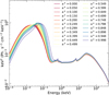 |
Fig. A.1. Spectra for different BH spin values a*. Other parameters are Ltransf/Ldisc = 0.5, h = 10 rg, MBH = 5 × 10⁷ M⊙, ṁEdd = 0.1, θ = 40°, Γ = 2, and Ecut, obs = 300 keV. |
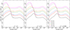 |
Fig. A.2. Spectra for different BH masses, MBH, considering spin values of a* = 0, 0.9, and 0.998 (left, middle, and right panels, respectively). Other parameters are Ltransf/Ldisc = 0.5, h = 10 rg, ṁEdd = 0.1, θ = 40°, Γ = 2, and Ecut, obs = 300 keV. |
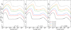 |
Fig. A.3. Spectra for different accretion rates, ṁEdd, considering spin values of a* = 0, 0.9, and 0.998 (left, middle, and right panels, respectively). Other parameters are Ltransf/Ldisc = 0.5, h = 10 rg, MBH = 5 × 10⁷ M⊙, θ = 40°, Γ = 2, and Ecut, obs = 300 keV. |
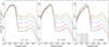 |
Fig. A.4. Spectra for different values of Ltransf/Ldisc, considering spin values of a* = 0, 0.9, and 0.998 (left, middle, and right panels, respectively). Other parameters are h = 10 rg, MBH = 5 × 10⁷ M⊙, ṁEdd = 0.1, θ = 40°, Γ = 2, and Ecut, obs = 300 keV. |
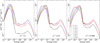 |
Fig. A.5. Spectra for different corona heights, h, considering spin values of a* = 0, 0.9, and 0.998 (left, middle, and right panels, respectively). Other parameters are Ltransf/Ldisc = 0.5, MBH = 5 × 10⁷ M⊙, ṁEdd = 0.1, θ = 40°, Γ = 2, and Ecut, obs = 300 keV. |
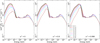 |
Fig. A.6. Spectra for different observer inclinations, θ, considering spin values of a* = 0, 0.9, and 0.998 (left, middle, and right panels, respectively). Other parameters are Ltransf/Ldisc = 0.5, h = 10 rg, MBH = 5 × 10⁷ M⊙, ṁEdd = 0.1, Γ = 2, and Ecut, obs = 300 keV. |
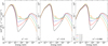 |
Fig. A.7. Spectra for different photon index values of the primary power-law X-ray component, Γ, considering spin values of a* = 0, 0.9, and 0.998 (left, middle, and right panels, respectively). Other parameters are Ltransf/Ldisc = 0.5 rg, h = 10 rg, MBH = 5 × 10⁷ M⊙, ṁEdd = 0.1, θ = 40° , and Ecut, obs = 300 keV. |
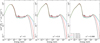 |
Fig. A.8. Spectra for different high energy cut-off values of the primary power-law X-ray component, Ecut, considering spin values of a* = 0, 0.9, and 0.998 (left, middle, and right panels, respectively). Other parameters are Ltransf/Ldisc = 0.5, h = 10 rg, MBH = 5 × 10⁷ M⊙, ṁEdd = 0.1, θ = 40° , and Γ = 2. |
All Tables
All Figures
|
Fig. 1. Dependence of Ltransf/Ldisc on the transition radius, rtrans. |
| In the text | |
|
Fig. 2. NT disc spectra (dashed red lines) and KYNSED disc SEDs with and without thermalisation (solid black lines and dotted blue lines, respectively) for a* = 0, 0.9 and 0.998 (left, middle, and right panel, respectively). The physical parameters are MBH = 5 × 10⁷ M⊙, Ltransf/Ldisc = 0.5, ṁEdd = 0.1, θ = 40°, h = 10 rg, Γ = 2, and Ecut, obs = 300 keV. |
| In the text | |
|
Fig. 3. Comparison between KYNSED and AGNSED (red) for a* = 0, 0.9, and 0.998 (left to right). The inclination is 40 degrees and Γ = 2 in both models. The dotted and solid black lines show the KYNSED model without the spectral hardening effect (colour-correction factor fcol = 1) and when the spectral hardening is computed following the Done et al. (2012) prescription (fcol = −1), respectively. |
| In the text | |
|
Fig. 4. Observed broadband NGC 5548 SED. The solid red line shows the model obtained for h = 46 rg. The dashed green line shows the unabsorbed best-fit model (i.e. by removing all Galactic and intrinsic neutral and warm absorbers). The dash-dotted black lines show the various spectral components. Empty circles indicate the data points that we did not consider during fitting, to avoid contamination from the BLR (see Sect. 4 for details). The grey, blue, and orange data points indicate the three X-ray spectra we used in the fitting. |
| In the text | |
|
Fig. 5. Best-fit parameters obtained by fitting the NGC 5548 broadband spectra for various corona heights. The vertical solid line and the grey shaded area indicate the best-fit value and the 1σ confidence range, respectively, of the height obtained by fitting the time-lag spectrum of this source with a* = 1 in K21b. The dashed black line in panel f shows the difference between the corona height and the event horizon, and the dotted blue line in the same panel shows the best-fit rtrans that corresponds to the fitted values of transferred energy, Ltransf/Ldisc, and black-hole spin, a*. |
| In the text | |
|
Fig. 6. Comparison of the primary X-ray spectra in the point source approximation used in KYNSED (black lines) with the 3D corona Monte Carlo computations of MONK (colour lines) for the spherical corona with different sizes, small (magenta), medium (blue), and large (yellow), at three heights. The three radii of the corona are Rc = 0.5, 1.5, and 2 rg for the height h = 3 rg; Rc = 1, 6, and 9 rg for the height h = 10 rg; and Rc = 5, 15, and 29 rg for the height h = 30 rg. The corona with the largest size extends as far as the BH horizon. The luminosities are divided by |
| In the text | |
|
Fig. A.1. Spectra for different BH spin values a*. Other parameters are Ltransf/Ldisc = 0.5, h = 10 rg, MBH = 5 × 10⁷ M⊙, ṁEdd = 0.1, θ = 40°, Γ = 2, and Ecut, obs = 300 keV. |
| In the text | |
|
Fig. A.2. Spectra for different BH masses, MBH, considering spin values of a* = 0, 0.9, and 0.998 (left, middle, and right panels, respectively). Other parameters are Ltransf/Ldisc = 0.5, h = 10 rg, ṁEdd = 0.1, θ = 40°, Γ = 2, and Ecut, obs = 300 keV. |
| In the text | |
|
Fig. A.3. Spectra for different accretion rates, ṁEdd, considering spin values of a* = 0, 0.9, and 0.998 (left, middle, and right panels, respectively). Other parameters are Ltransf/Ldisc = 0.5, h = 10 rg, MBH = 5 × 10⁷ M⊙, θ = 40°, Γ = 2, and Ecut, obs = 300 keV. |
| In the text | |
|
Fig. A.4. Spectra for different values of Ltransf/Ldisc, considering spin values of a* = 0, 0.9, and 0.998 (left, middle, and right panels, respectively). Other parameters are h = 10 rg, MBH = 5 × 10⁷ M⊙, ṁEdd = 0.1, θ = 40°, Γ = 2, and Ecut, obs = 300 keV. |
| In the text | |
|
Fig. A.5. Spectra for different corona heights, h, considering spin values of a* = 0, 0.9, and 0.998 (left, middle, and right panels, respectively). Other parameters are Ltransf/Ldisc = 0.5, MBH = 5 × 10⁷ M⊙, ṁEdd = 0.1, θ = 40°, Γ = 2, and Ecut, obs = 300 keV. |
| In the text | |
|
Fig. A.6. Spectra for different observer inclinations, θ, considering spin values of a* = 0, 0.9, and 0.998 (left, middle, and right panels, respectively). Other parameters are Ltransf/Ldisc = 0.5, h = 10 rg, MBH = 5 × 10⁷ M⊙, ṁEdd = 0.1, Γ = 2, and Ecut, obs = 300 keV. |
| In the text | |
|
Fig. A.7. Spectra for different photon index values of the primary power-law X-ray component, Γ, considering spin values of a* = 0, 0.9, and 0.998 (left, middle, and right panels, respectively). Other parameters are Ltransf/Ldisc = 0.5 rg, h = 10 rg, MBH = 5 × 10⁷ M⊙, ṁEdd = 0.1, θ = 40° , and Ecut, obs = 300 keV. |
| In the text | |
|
Fig. A.8. Spectra for different high energy cut-off values of the primary power-law X-ray component, Ecut, considering spin values of a* = 0, 0.9, and 0.998 (left, middle, and right panels, respectively). Other parameters are Ltransf/Ldisc = 0.5, h = 10 rg, MBH = 5 × 10⁷ M⊙, ṁEdd = 0.1, θ = 40° , and Γ = 2. |
| In the text | |
Current usage metrics show cumulative count of Article Views (full-text article views including HTML views, PDF and ePub downloads, according to the available data) and Abstracts Views on Vision4Press platform.
Data correspond to usage on the plateform after 2015. The current usage metrics is available 48-96 hours after online publication and is updated daily on week days.
Initial download of the metrics may take a while.