| Issue |
A&A
Volume 660, April 2022
|
|
|---|---|---|
| Article Number | A33 | |
| Number of page(s) | 7 | |
| Section | Stellar structure and evolution | |
| DOI | https://doi.org/10.1051/0004-6361/202142696 | |
| Published online | 05 April 2022 | |
Rieger-type cycles on the solar-like star KIC 2852336
1
Georg-August-Universität, Institut für Astrophysik, Friedrich-Hund-Platz 1, 37077 Göttingen, Germany
2
School of Natural Sciences and Medicine, Ilia State University, Cholokashvili ave. 3/5, Tbilisi, Georgia
e-mail: This email address is being protected from spambots. You need JavaScript enabled to view it.
3
E. Kharadze Georgian National Astrophysical Observatory, Mount Kanobili, Georgia
4
Institute of Physics, IGAM, University of Graz, Universitätsplatz 5, 8010 Graz, Austria
5
Max-Planck-Institut für Sonnensystemforschung, Justus-von-Liebig-Weg 3, 37077 Göttingen, Germany
6
INAF-Osservatorio Astrofisico di Catania, Via S. Sofia, 78, 95123 Catania, Italy
Received:
18
November
2021
Accepted:
24
January
2022
Abstract
Context. A Rieger-type periodicity of 150–180 days (six to seven times the solar rotation period) has been observed in the Sun’s magnetic activity and is probably connected with the internal dynamo layer. Observations of Rieger cycles in other solar-like stars may give us information about the dynamo action throughout stellar evolution.
Aims. We aim to use the Sun as a star analogue to find Rieger cycles on other solar-like stars using Kepler data.
Methods. We analyse the light curve of the Sun-like star KIC 2852336 (with a rotation period of 9.5 days) using wavelet and generalised Lomb-Scargle methods to find periodicities over rotation and Rieger timescales.
Results. Besides the rotation period of 9.5 days, the power spectrum shows a pronounced peak at a period of 61 days (about six times the stellar rotation period) and a less pronounced peak at 40–44 days. These two periods may correspond to Rieger-type cycles and can be explained by the harmonics of magneto-Rossby waves in the stellar dynamo layer. The observed periods and theoretical properties of magneto-Rossby waves lead to the estimation of the dynamo magnetic field strength of 40 kG inside the star.
Conclusions. Rieger-type cycles can be used to probe the dynamo magnetic field in solar-type stars at different phases of evolution. Comparing the rotation period and estimated dynamo field strength of the star KIC 2852336 with the corresponding solar values, we conclude that the ratio Ω/BD, where Ω is the angular velocity and BD is the dynamo magnetic field, is the same for the star and the Sun. Therefore, the ratio can be conserved during stellar evolution, which is consistent with earlier observations that younger stars are more active.
Key words: stars: activity / stars: magnetic field / stars: solar-type / stars: rotation / starspots
© ESO 2022
1. Introduction
Solar activity has its main periodicity at about 11 years, which is known as Schwabe cycle (Schwabe 1844). However, the Sun also shows shorter-period variations of 150–180 days (Rieger et al. 1984) that usually appear near solar cycle maxima in the activity indices, which are connected to the global magnetic field (Bai & Sturrock 1987; Lean & Brueckner 1989; Carbonell & Ballester 1990; Oliver et al. 1998). Such a periodicity is probably related to the solar internal dynamo layer, where the large-scale magnetic field is generated. The periodicity was recently explained by magneto-Rossby waves in the dynamo layer, which may lead to the quasi-periodic eruption of magnetic flux towards the surface and hence to the modulation of solar activity (Zaqarashvili et al. 2010, 2021). Therefore, observed periods and theoretical dispersion relations of Rossby waves can lead to the estimation of the solar dynamo field strength (Gurgenashvili et al. 2016; Zaqarashvili & Gurgenashvili 2018). Using the solar and stellar analogy, similar short-term oscillations in stellar activity can be used to estimate the magnetic field strength in the dynamo layers of stars at different stages of evolution.
To search for Schwabe cycles on other stars, Wilson (1968) started to measure the emission in the Ca II H + K line cores, now known as the Mount Wilson S-index. First results of the measurements showed that several of the 91 targeted main sequence stars displayed cyclic activity (Wilson 1978). Baliunas et al. (1995) studied the Ca II H & K flux of 111 stars and reported that almost 52 of them showed cycling activity1. On the other hand, Baliunas et al. (1997) reported the first detection of short-term periodic variations in other Sun-like stars. After studying three stars, ρ1 Cancri (Prot = 42 days, age 5 Gyr), τ Bootis (Prot = 3.3 days, age 2 Gyr, F7 dwarf), and ν Andromedae (Prot = 12 days, age 5 Gyr), Baliunas et al. (1997) found a short cycle of 116 days in τ Bootis, which persisted for 30 years. Recently, Mittag et al. (2017), Mengel et al. (2016), and Schmitt & Mittag (2017) observed 120-, 117-, and 90-day variations in the same star. Mittag et al. (2019) found four other F-type stars with rotation periods of 3.45 to 7.73 days that display short-term cycles with periods of < 1 yr.
The recent NASA space missions Kepler (Borucki et al. 2010) and the Transiting Exoplanet Survey Satellite (TESS; Ricker et al. 2014) as well as the Centre National D’Etudes Spatiales and European Space Agency (CNES/ESA) mission Convection, Rotation and planetary Transits (CoRoT; Baglin et al. 2008) collected a great deal of information about other solar-like stars. These missions provide light curves, which can be modulated by starspots and hence lead to the determination of stellar rotation (Nielsen et al. 2013; Reinhold et al. 2013; McQuillan et al. 2014). Periodic variations of starspots due to activity cycles can also be revealed via light curve analysis (Reinhold et al. 2017; Arkhypov et al. 2015). However, space mission data allow only short-term cycles to be detected due to the relatively short observation intervals compared to Mount Wilson data. Mathur et al. (2014) studied the activity of 22 F-type stars and reported that only two of them showed 1400- and 650-day hints of activity cycles. Ferreira Lopes et al. (2015) analysed the CoRoT main sequence FGK-type stars and found stellar cycles ranging from 33 to 650 days.
Some Kepler and CoRoT Sun-like stars show short-term variations that are probably similar to the solar Rieger cycles (Lanza 2010). The Rieger-type cycle (PR) is six to seven times longer than the rotation period of the Sun (Prot is ≈26 days and the Rieger type periodicity is around 150–180 days). Lanza et al. (2009) studied the star CoRoT-2, which has a rotation period of 4.52 days and showed an additional periodicity of 29 days in its light curve, which may be analogous to the Rieger cycle. Bonomo & Lanza (2012) found a periodicity of 48 days in the light curves of the star Kepler-17 with Prot = 12 days, which could also correspond to the Rieger period. Recently, Lanza et al. (2019) re-analysed the light curves of the same star for all Kepler quarters and found an additional cycle of 400–500 days. Arkhypov & Khodachenko (2021) studied 1726 Kepler stars and found two types of Rieger cycles: one independent of the stellar Prot (for the stars with Teff ≲ 5500 K) and the other proportional to Prot (for the stars with Teff ≳ 6300 K). Therefore, it is becoming increasingly clear that space mission data may reveal Rieger cycles in the activity of other solar-like stars.
The Sun is a slowly rotating star with an equatorial period of around 26 days. Observations show that young solar-type stars rotate much faster than the present Sun. As a consequence, young solar-type stars may have vigorous magnetic dynamos and consequently strong magnetic activity. The young stars lose angular momentum via magnetised stellar winds (Mestel 1968), and therefore their rotation slows down with age (Skumanich 1972). As a response to slower rotation, the stellar dynamo also weakens with time, causing stellar activity to undergo a significant decrease (Ribas et al. 2005; Lammer et al. 2012). The stellar differential rotation may also change during the stellar evolution (Metcalfe & van Saders 2017). With the recent Kepler mission, the rotation rate of thousands of stars was estimated (Nielsen et al. 2013; Reinhold et al. 2013; McQuillan et al. 2014).
Recently, Gurgenashvili et al. (2021) analysed the total irradiance of the Sun as a star to detect the Rieger-type periodicity. These authors found a clear signature of Rieger cycles, which was used to estimate the magnetic field strength in the dynamo layer. Inspired by the results of that work, we analyse the light curves of Kepler star KIC 2852336 to search for Rieger periodicity and attempt to probe the dynamo magnetic field in the stellar interior. Due to some restrictions, detecting a star with noticeable different periods other than the Prot is quite challenging in Kepler data. Most frequently, only rotation periods are observed in Kepler periodograms. The longer periods need to be rigorously checked as, for the most part, they might be false, instrumental, or affected by multiple events and may not belong to stellar activity.
2. Data and methods
Several catalogues have been created from long-term Kepler data using automated methods. Nielsen et al. (2013) searched for rotation periods in more than 150 000 main sequence stars for Kepler quarters 2 to 9 (the online catalogue can be found at the CDS2). They found reliable Prot values for 12 151 stars. Reinhold et al. (2013) analysed the light curves for 40 661 active Kepler stars from quarter 3 and found stable rotation periods between 0.5 and 45 days for 24 124 stars (the catalogue can also be found at the CDS3).
McQuillan et al. (2014) determined the rotation periods of more than 34 000 stars for quarters 3 to 14 and divided stellar populations into two different groups: fast-rotating young stars and slow-rotating old stars. The McQuillan catalogue4 also includes 99 000 stars whose rotation periods could not be determined for various reasons. The Sun-like stars from this catalogue can be selected using different criteria. The first physical characteristic is the effective surface temperature, Teff (5778 K for the Sun). The second characteristic is the surface gravity, logg (which is 4.2 for the Sun). Therefore, the target stars should have similar values. The third characteristic is a rotation period, which varies between 0.5 and 70 days in this catalogue. To study the periodicity in the light curve of the star, we used a generalised Lomb-Scargle (GLS) periodogram, which is adequate for unevenly spaced data (Zechmeister & Kürster 2009) and the wavelet transform (Torrence & Compo 1998).
There are two types of Kepler data: Simple Aperture Photometry (SAP) and Pre-search Data Conditioning (PDC) time series. SAP data are corrected only for the background flux and contain strong instrumental trends. Therefore, some additional corrections are needed to avoid systematics of instrumental origin. In PDC data, instrumental trends are mostly removed, and they are obtained after correction for the common trends shown by stars of similar magnitude and position on the same charge-coupled device (CCD) as the target. PDC data are sometimes strongly affected by the aggressive method used to correct for the instrumental trends, and all the variability on timescales longer than about 20–25 days is strongly reduced or suppressed, especially by the so-called multi-scale maximum a posteriori (msMAP) approach (Gilliland et al. 2015). So periods detected in the Kepler PDC data are probably very strong as they survived the correction process. Here we used the PDC data.
When the star moves from one CCD to another in the Kepler focal plane, the raw data display jumps from one quarter to the other, which can produce ugly effects in the computation of the GLS periodogram or Morlet wavelet. Therefore, we first had to remove these effects, which can be done by matching the median values between successive quarters. There are also gaps in the data of up to several days, and sometimes even several months, between the quarters, depending on the location of the stars on the Kepler focal plane. These gaps could be problematic during data analysis. The GLS works well with the unevenly spaced data; however, the Morlet wavelet needs evenly spaced data. One method to address this is to fill the gap with averages. We first calculated the daily averages and then filled the gaps using those averages.
We are interested in searching for the PR; therefore, we looked for periods of five to seven times the rotation period. Reliable oscillations in Kepler data can be found only with a period of < 90 days (one quarter in the Kepler time series). As such, we concentrated on stars with rotation periods of 5–15 days (younger analogues of the Sun).
Power spectra of Kepler stars normally show very pronounced peaks at the periods around Prot and Prot/2. Longer periodicity is not usually seen unless one removes the peaks corresponding to stellar rotation. Finding a star with pronounced periods other than the Prot is quite difficult in Kepler data. During the search for Sun-like stars with Rieger-type cycles in Kepler data, we found the star KIC 2852336, which showed pronounced periodicity near Rieger timescales. Therefore, we started to analyse the light curves of the star in detail. The star has Teff = 5601 K and logg = 4.906 according to the McQuillan catalogue. Slightly different measurements can be found in Mathur et al. (2017) 5, with Teff = 5809, logg = 4.56, and [Fe/H]= − 0.26. This star was also found in the Gaia archive (with ID Gaia DR2 2052578412798483072)6 and TESS input catalogue (TIC 137149729)7. The basic parameters of the star are presented in Table 1.
Basic parameters of the star KIC 2852336 in the Kepler (rows 1 – 2), TESS (third row), and Gaia (last row) data archives.
Periods in Kepler data, which are longer than the rotation periods, need additional verification that they belong to stellar activity. First of all, one should exclude the existence of a companion star or the possibility of a multiple system. Kepler is limited to about 16 magnitudes and hence cannot detect stars that are much fainter. Our target star might have a fainter companion that stays beyond Kepler resolution. To exclude the influence of a faint companion or background star, we checked the Gaia data for stars in the vicinity of KIC 2852336. Gaia data contain stars that are 5 mag fainter than the Kepler stars. We checked the Gaia archive using the same coordinates and could not find any companion within a radius of 11 arcsec, which indicates that this period is not caused by a companion star.
3. Rieger-type periodicity
The light curve of KIC 2852336 (upper panel of Fig. 1) shows a clear rotational modulation of around 9.5 days. The solid black line denotes the 20-day moving average, showing modulation of around 60–61 days. The lower panel of Fig. 1 displays a significant peak at the period of 58–61 days, which corresponds to the timescale of Rieger-type periodicity. The Kepler data have been cleaned several times, eliminating instrumental effects or the effects of cosmic rays and the various types of noise, and therefore this period is probably not instrumental. However, it still needs to be carefully checked to verify that the period really characterises stellar activity.
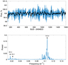 |
Fig. 1. Time series of the Kepler star KIC 2852336 with solid black line denoting the 20-day moving average (upper panel) and the corresponding GLS power spectrum (lower panel). The frequency interval, which includes the periods between 1–90 days, is presented; the rotational periods of 9.5 d, 44 d and 58–61 d (indicated by black arrows), which may correspond to the Rieger cycle, are clearly seen. |
Kepler data have some pronounced instrumental timescales, for example 30 and 90 days. For instance, every 30 days Kepler makes small adjustments to the spacecraft to send data to the ground by first re-pointing its radio antenna. Every 90 days (a time interval called a quarter in the Kepler jargon), the spacecraft (and therefore the focal plane) is rotated by 90 degrees. As the spacecraft rotates, a star jumps to another CCD with a different sensitivity and different settings than the previous one. The star returns to the same CCD in every fourth quarter. Therefore, if we see the same period in every fourth quarter only, we can assume that this period is instrumental (provoked by CCD settings) and therefore unreliable.
Figure 2 shows the Morlet wavelet spectrum of the light curve variations during the entire four years of Kepler observations. The rotation period is continuously seen during the whole interval, with more power in some quarters. The period of 61 days is also very well observed during all the observations. The right panel of the figure shows the power spectrum in the period interval of 20–90 days, which allows us to visualise the variation in this periodicity over time. The periodicity is seen in all quarters, which clearly shows that it is not CCD dependent.
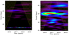 |
Fig. 2. Morlet wavelet analysis of light curve variations during entire Kepler observations. Left panel: spectrum of the periods between 1 and 90 days, and the right panel shows the periods between 20 and 90 days (Prot is removed). The hatched regions in the figure show the cone of influence, which means that the wavelet transform is not reliable in these areas. |
We performed another analysis to prove that the periodicity is not instrumental. We chose several stars nearby our target star with similar magnitude, effective temperature, and surface gravity and followed the same path across the Kepler CCDs. The Kepler space telescope is a Schmidt telescope composed of 21 Science CCD modules and four fine guidance sensor CCD modules. Each Science CCD module consists of two 50 × 25 mm 2200 × 1024 pixel CCDs. Each Science module has four independent outputs and channels (for a total of 84 channels). We searched for these closest stars in all of the 17 quarters. The stars would be very close to our star if they fell on exactly the same CCD, same module, and same channel. If the other stars had the same periodicity in light curves, then the periodicity would be instrumental.
We found ten solar-type stars close to our star (see the stellar parameters in Table 2). Then we performed the GLS analysis of stellar light curves one by one. None of these stars had a peak around the period of 61 days. Figure 3 shows the GLS periodograms of four different stars from the above sample. This figure shows that the stars have very strong amplitudes at Prot, but any other periodicity is absent. Therefore, we are confident that the period of 58–61 days in the light curve of our target star is a real periodicity and corresponds to the Rieger cycle.
Selected solar-type stars in the neighbourhood of our target star.
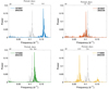 |
Fig. 3. GLS periodograms of four Sun-like stars in the neighbourhood of the target star, marked with different colours. The thin grey line shows the periodogram of our target star for comparison. |
Besides the period of 60 days, GLS and wavelet analyses show another period near 40–45 days (see Figs. 1 and 2). The period has less power than the period of 58–61 days, but it is still seen on the power spectra. All the above analyses that ruled out instrumental effects are relevant to this period as well.
Solar Rieger-type periodicity is explained by magneto-Rossby waves in the dynamo layer, where the magnetic flux is periodically modulated by the waves and the quasi-periodic eruption of the flux towards the surface is triggered (Zaqarashvili et al. 2010, 2021). Then, due to the same mechanism, magneto-Rossby waves in the dynamo layer of our star may lead to the quasi-periodic modulation of magnetic structures on the stellar surface and therefore the modulation of the light curve.
In Fig. 4, we plot the period versus dynamo magnetic field strength for magneto-Rossby wave modes with m = 1 and n = 3, 4 according to Eq. (43) from Gachechiladze et al. (2019), where m and n are the angular order and degree of spherical harmonics, respectively. We see that a dynamo magnetic field with a strength of 40 kG yields the observed periods of 61 days and 44 days for the harmonics of n = 4 and n = 3, respectively.
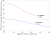 |
Fig. 4. Period of magneto-Rossby waves vs. dynamo magnetic field strength. Here the red (blue) curve corresponds to the spherical harmonic with m = 1 and n = 4 (n = 3), where m and n are the angular order and degree. |
4. Discussion and conclusion
Detailed information about the Sun gathered over centuries can be used to study stellar atmospheres and interiors. On the other hand, recent space missions have collected a huge amount of information about many solar-like stars, though uncovering detailed processes in individual stars is not easy. Therefore, solar processes can be used to model the stellar atmosphere and interior, while solar-like stars at different stages of evolution can be used to study the time evolution of the Sun.
A Rieger-type periodicity of 155–180 day is an interesting observational feature seen in many indices of solar activity. The periodicity is probably connected with magneto-Rossby waves in the solar dynamo layer below the convection zone (Zaqarashvili et al. 2010, 2021). Therefore, observations and theoretical properties of the waves can be used to probe the layer, namely to estimate the dynamo field strength (Gurgenashvili et al. 2016, 2017; Zaqarashvili & Gurgenashvili 2018). Total irradiance of the Sun is comparable to stellar light curves, and therefore it is important to first look into Rieger-type periodicity in the irradiance. Gurgenashvili et al. (2021) studied the total solar irradiance during solar cycles 23 and 24 and found two distinct periods of 185 days and 115 days (in cycle 23) and 170 and 145 days (in cycle 24), which led to the estimation of the dynamo field strength as 10–15 kG. It is thus important to perform a similar analysis on solar-type stars and compare the results to those of the Sun.
We analysed the light curve of the Kepler star KIC 2852336 (Prot = 9.5 days), which is a young analogue of the Sun. We found a very clear period of 58–61 days in the power spectrum of stellar light curve oscillations, which is the timescale of Rieger-type periodicity for the star. We used different methods to confirm that this periodicity is a real variation of stellar irradiance and not instrumental or from some other source. First, we checked for the existence of faint companion stars with the same coordinates in the Gaia archive but found that this star has no companion within a radius of 11 arcsec. Second, we checked whether the period is provoked by particular CCD settings (due to the spacecraft rotation, the star returns to the same CCD in every fourth quarter, i.e. every 90 days). However, the periodicity is seen during whole observations (Fig. 2), and therefore CCD dependence is also ruled out. Third, we checked other stars with similar magnitudes, temperatures, and surface gravity from exactly the same CCD channel. Light curves of several stars did not display any indication of 58–61 day and 40–44 day periods, which confirmed that the periodicity in our target star really corresponds to its activity. There might be several reasons for the absence of clear Rieger cycles on those stars. First, stars might be tilted such that only polar regions are observed from the Earth. If spots (and structures associated with strong magnetic fields) appear near equatorial regions like on the Sun, then they will not affect the stellar light curve. Second, Kepler observations lasted only 4 years, a time span in which many stars do not complete an entire activity cycle. Rieger periodicity on the Sun appears only near activity maximum; therefore, if a star is in its minimum phase, then it will not show the Rieger periodicity. Third, Rieger-type cycles might exist in some stars but not be visible due to weak peaks in the power spectrum. Below we discuss several consequences of our analysis, which may become important points in stellar evolution.
One important aspect in stellar evolution is connected with the stellar magnetic field, which governs activity in the form of starspots, stellar flares, and coronal mass ejections. The magnetic field of solar-type stars is believed to be amplified in the dynamo layer below or inside the convection zone. The magnetic flux rises towards the surface owing to the magnetic buoyancy and appears in the form of starspots. It is known that younger stars show faster rotation and the rotation period rate decreases with age (Skumanich 1972; Lammer et al. 2012). One plausible mechanism for this slowdown is the magnetic breaking when the stellar wind flowing along the magnetic field lines takes the angular momentum from stars (Mestel 1968). Therefore, magnetic field evolution throughout the main sequence is an important factor in stellar life. To understand the magnetic field evolution process, it is of vital importance to know the dynamo field strength at different stages of stellar evolution. The field strength in the stellar dynamo layer can be estimated via asteroseismology, but it is a difficult task. Therefore, even a rough estimation of the dynamo field strength in stellar interiors may become a key point in understanding stellar magnetic evolution.
The most plausible mechanism for Rieger-type periodicity is magneto-Rossby waves in the solar dynamo layer, which lead to the modulation of the dynamo field and consequently trigger the quasi-periodic eruption of magnetic flux towards the surface (Zaqarashvili et al. 2010). Therefore, the observed periods and dispersion relation of magneto-Rossby waves can be used to estimate the dynamo magnetic field strength (Gurgenashvili et al. 2016, 2017; Zaqarashvili & Gurgenashvili 2018). Gurgenashvili et al. (2021) analysed the total solar irradiance data for solar cycles 23 and 24 and found the existence of periods of 185 and 115 days and 170 and 145 days, respectively, which were explained as being due to the spherical harmonics of magneto-Rossby waves with m = 1 and n = 4, 3. Consequently, a magnetic field of ∼10–15 kG was estimated in the solar dynamo layer. The periods in the light curve of the target star are found to be around 58–61 days and 40–44 days, which satisfy the same ratio of PR/Prot as for the Sun. Figure 4 shows that a dynamo field strength of 40 kG yields the observed periods for the magneto-Rossby wave harmonics with m = 1 and n = 4, 3. Therefore, the estimated dynamo field in our target star is three times stronger than that of the Sun estimated with the same method (Gurgenashvili et al. 2021). The rotation period of the target star (9.5 days) is also three times smaller than the rotation period of the Sun (27 days). Therefore, a comparison of the rotation periods and estimated dynamo magnetic field strengths of our star and the Sun shows an interesting ratio,
 (1)
(1)
which can be rewritten as
 (2)
(2)
where Ω is the stellar angular velocity and BD is the dynamo magnetic field strength. Equation (2) shows that the dynamo magnetic field is proportional to the rotation during stellar evolution, and therefore young fast-rotating solar-type stars should show a stronger field and hence stronger magnetic activity. This has long been known, and therefore our result agrees with other observations (for a theoretical discussion, see e.g. Durney & Robinson 1982). The advantage of Eq. (2) is that one can estimate the dynamo field from the stellar rotation period. However, Eq. (2) is obtained from the analyses of the Sun and one other star and could therefore be just coincidence. More stellar samples are required to confirm it.
Acknowledgments
EG was supported by Shota Rustaveli National Science Foundation of Georgia (SRNSFG) [grant number N04/46, project number N93569] and by Volkswagen Foundation in the framework of the joint project “Structured Education Quality Assurance Freedom to Think”. TVZ was supported by the Austrian Fonds zur Förderung der Wissenschaftlichen Forschung (FWF) project P30695-N27. TR acknowledges support from the European Research Council (ERC) under the European Union’s Horizon 2020 research and innovation program (grant agreement No. 715947). This paper resulted from discussions at workshops of ISSI (International Space Science Institute) team (ID 389) “Rossby waves in astrophysics” organised in Bern (Switzerland).
References
- Arkhypov, O. V., & Khodachenko, M. L. 2021, A&A, 651, A28 [NASA ADS] [CrossRef] [EDP Sciences] [Google Scholar]
- Arkhypov, O. V., Khodachenko, M. L., Lammer, H., et al. 2015, ApJ, 807, 109 [NASA ADS] [CrossRef] [Google Scholar]
- Bai, T., & Sturrock, P. A. 1987, Nature, 327, 601 [NASA ADS] [CrossRef] [Google Scholar]
- Baglin, A., Auvergne, M., Barge, P., Deleuil, M., & Michel, E. 2008, Proc. Int. Astron. Union, 4, 71 [NASA ADS] [CrossRef] [Google Scholar]
- Baliunas, S. L., Donahue, R. A., Soon, W. H., et al. 1995, ApJ, 438, 269 [Google Scholar]
- Baliunas, S. L., Henry, G. W., Donahue, R. A., Fekel, F. C., & Soon, W. H. 1997, ApJ, 474, L119 [NASA ADS] [CrossRef] [Google Scholar]
- Bonomo, A. S., & Lanza, A. F. 2012, A&A, 547, A37 [NASA ADS] [CrossRef] [EDP Sciences] [Google Scholar]
- Borucki, W., Koch, D., Basri, G., Batalha, N., et al. 2010, Science, 327, 977 [CrossRef] [PubMed] [Google Scholar]
- Carbonell, M., & Ballester, J. L. 1990, A&A, 238, 377 [NASA ADS] [Google Scholar]
- Durney, B. R., & Robinson, R. D. 1982, ApJ, 253, 290 [NASA ADS] [CrossRef] [Google Scholar]
- Ferreira Lopes, C. E., Le ao, I. C., de Freitas, D. B., et al. 2015, A&A, 583, A134 [NASA ADS] [CrossRef] [EDP Sciences] [Google Scholar]
- Gachechiladze, T., Zaqarashvili, T. V., Gurgenashvili, E., et al. 2019, ApJ, 874, 162 [NASA ADS] [CrossRef] [Google Scholar]
- Gurgenashvili, E., Zaqarashvili, T. V., Kukhianidze, V., et al. 2016, ApJ, 826, 55 [NASA ADS] [CrossRef] [Google Scholar]
- Gurgenashvili, E., Zaqarashvili, T. V., Kukhianidze, V., et al. 2017, ApJ, 845, 137 [NASA ADS] [CrossRef] [Google Scholar]
- Gurgenashvili, E., Zaqarashvili, T. V., Kukhianidze, V., et al. 2021, A&A, 653, A146 [NASA ADS] [CrossRef] [EDP Sciences] [Google Scholar]
- Gilliland, R. L., Chaplin, W. J., Jenkins, J. M., Ramsey, L. W., & Smith, J. C. 2015, AJ, 150, 133 [Google Scholar]
- Lanza, A. F. 2010, in Stellar Magnetic Cycles, eds. A. G. Kosovichev, A. H. Andrei, & J. P. Roelot, IAU Symp., 264, 120 [NASA ADS] [Google Scholar]
- Lanza, A. F., Pagano, I., Leto, G., et al. 2009, A&A, 493, 193 [NASA ADS] [CrossRef] [EDP Sciences] [Google Scholar]
- Lanza, A. F., Netto, Y., Bonomo, A. S., et al. 2019, A&A, 626, A38 [NASA ADS] [CrossRef] [EDP Sciences] [Google Scholar]
- Lammer, H., Güdel, M., Kulikov, Y., et al. 2012, Earth Planets Space, 64, 179 [NASA ADS] [CrossRef] [Google Scholar]
- Lean, J. L., & Brueckner, G. E. 1989, ApJ, 337, 568 [Google Scholar]
- Mathur, S., García, R. A., Ballot, J., et al. 2014, A&A, 562, A124 [NASA ADS] [CrossRef] [EDP Sciences] [Google Scholar]
- Mathur, S., Huber, D., Batalha, N. M., et al. 2017, ApJS, 229, 30 [NASA ADS] [CrossRef] [Google Scholar]
- McQuillan, A., Mazeh, T., & Aigrain, S. 2014, ApJS, 211, 24 [Google Scholar]
- Mittag, M., Robrade, J., Schmitt, J. H. M. M., et al. 2017, A&A, 600, A119 [NASA ADS] [CrossRef] [EDP Sciences] [Google Scholar]
- Mittag, M., Schmitt, J. H. M. M., Hempelmann, A., & Schroeder, K.-P. 2019, A&A, 621, A136 [NASA ADS] [CrossRef] [EDP Sciences] [Google Scholar]
- Mengel, M. W., Fares, R., Marsden, S. C., et al. 2016, MNRAS, 459, 4325 [NASA ADS] [CrossRef] [Google Scholar]
- Mestel, L. 1968, MNRAS, 138, 359 [NASA ADS] [CrossRef] [Google Scholar]
- Metcalfe, T. S., & van Saders, J. 2017, Sol. Phys., 292, 126 [NASA ADS] [CrossRef] [Google Scholar]
- Nielsen, M. B., Gizon, L., Schunker, H., & Karoff, C. 2013, A&A, 557, L10 [NASA ADS] [CrossRef] [EDP Sciences] [Google Scholar]
- Oliver, R., Ballester, J. L., & Boudin, F. 1998, Nature, 394, 552 [NASA ADS] [CrossRef] [Google Scholar]
- Ribas, I., Guinan, E. F., Güdel, M., & Audard, M. 2005, ApJ, 622, 680 [Google Scholar]
- Ricker, G. R., Winn, J. N., Vanderspek, R., et al. 2014, Proc. SPIE, 9143 [Google Scholar]
- Rieger, E., Share, G. H., Forrest, D. J., Kanbach, G., Reppin, C., et al. 1984, Nature, 312, 623 [NASA ADS] [CrossRef] [Google Scholar]
- Reinhold, T., Reiners, A., & Basri, G. 2013, A&A, 560, A4 [NASA ADS] [CrossRef] [EDP Sciences] [Google Scholar]
- Reinhold, T., Cameron, R. H., & Gizon, L. 2017, A&A, 603, A52 [NASA ADS] [CrossRef] [EDP Sciences] [Google Scholar]
- Skumanich, A. 1972, ApJ, 171, 565 [Google Scholar]
- Schmitt, J. H. M. M., & Mittag, M. 2017, A&A, 600, A120 [NASA ADS] [CrossRef] [EDP Sciences] [Google Scholar]
- Schwabe, H. 1844, Astron. Nachr., 21, 233 [Google Scholar]
- Torrence, C., & Compo, G. P. 1998, BAMS, 79, 61 [NASA ADS] [CrossRef] [Google Scholar]
- Wilson, O. C. 1968, ApJ, 153, 221 [Google Scholar]
- Wilson, O. C. 1978, ApJ, 226, 379 [Google Scholar]
- Zaqarashvili, T. V., & Gurgenashvili, E. 2018, Front. Astron. Space Sci., 5, 7 [CrossRef] [Google Scholar]
- Zaqarashvili, T. V., Carbonell, M., Oliver, R., & Ballester, J. L. 2010, ApJ, 709, 749 [NASA ADS] [CrossRef] [Google Scholar]
- Zaqarashvili, T. V., Albekioni, M., Ballester, J. L., et al. 2021, Space Sci. Rev., 217, 15 [Google Scholar]
- Zechmeister, M., & Kürster, M. 2009, A&A, 496, 577 [CrossRef] [EDP Sciences] [Google Scholar]
All Tables
Basic parameters of the star KIC 2852336 in the Kepler (rows 1 – 2), TESS (third row), and Gaia (last row) data archives.
All Figures
|
Fig. 1. Time series of the Kepler star KIC 2852336 with solid black line denoting the 20-day moving average (upper panel) and the corresponding GLS power spectrum (lower panel). The frequency interval, which includes the periods between 1–90 days, is presented; the rotational periods of 9.5 d, 44 d and 58–61 d (indicated by black arrows), which may correspond to the Rieger cycle, are clearly seen. |
| In the text | |
|
Fig. 2. Morlet wavelet analysis of light curve variations during entire Kepler observations. Left panel: spectrum of the periods between 1 and 90 days, and the right panel shows the periods between 20 and 90 days (Prot is removed). The hatched regions in the figure show the cone of influence, which means that the wavelet transform is not reliable in these areas. |
| In the text | |
|
Fig. 3. GLS periodograms of four Sun-like stars in the neighbourhood of the target star, marked with different colours. The thin grey line shows the periodogram of our target star for comparison. |
| In the text | |
|
Fig. 4. Period of magneto-Rossby waves vs. dynamo magnetic field strength. Here the red (blue) curve corresponds to the spherical harmonic with m = 1 and n = 4 (n = 3), where m and n are the angular order and degree. |
| In the text | |
Current usage metrics show cumulative count of Article Views (full-text article views including HTML views, PDF and ePub downloads, according to the available data) and Abstracts Views on Vision4Press platform.
Data correspond to usage on the plateform after 2015. The current usage metrics is available 48-96 hours after online publication and is updated daily on week days.
Initial download of the metrics may take a while.