| Issue |
A&A
Volume 660, April 2022
|
|
|---|---|---|
| Article Number | A30 | |
| Number of page(s) | 12 | |
| Section | Stellar structure and evolution | |
| DOI | https://doi.org/10.1051/0004-6361/202142289 | |
| Published online | 05 April 2022 | |
New simulations of accreting DA white dwarfs: Inferring accretion rates from the surface contamination
1
Instituto de Astrofísica de La Plata (UNLP – CONICET), Facultad de Ciencias Astronómicas y Geofísicas, Universidad Nacional de La Plata, La Plata, Argentina
e-mail: This email address is being protected from spambots. You need JavaScript enabled to view it.
2
Université de Toulouse, UPS-OMP, IRAP, Toulouse, France
3
CNRS, IRAP, 14 avenue Edouard Belin, 31400 Toulouse, France
Received:
22
September
2021
Accepted:
15
December
2021
Abstract
Context. A non-negligible fraction of white dwarf stars show the presence of heavy elements in their atmospheres. The most accepted explanation for this contamination is the accretion of material coming from tidally disrupted planetesimals, which forms a debris disk around the star.
Aims. We provide a grid of models for hydrogen-rich white dwarfs accreting heavy material. We sweep a 3D parameter space that has different effective temperatures, envelope hydrogen contents, and accretion rates. The grid is appropriate for determining accretion rates in white dwarfs that show the presence of heavy elements.
Methods. Full evolutionary calculations of accreting white dwarfs were computed including all relevant physical processes, particularly the fingering (thermohaline) convection, a process neglected in most previous works, which has to be considered to obtain realistic estimations. Accretion is treated as a continuous process, and bulk-Earth composition is assumed for the accreted material.
Results. We obtain final (stationary or near-stationary) and reliable abundances for a grid of models that represent hydrogen-rich white dwarfs of different effective temperatures and hydrogen contents, which we apply to various accretion rates.
Conclusions. Our results provide estimates of accretion rates, accounting for thermohaline mixing, to be used for further studies on evolved planetary systems.
Key words: white dwarfs / stars: evolution / stars: abundances / stars: interiors / accretion, accretion disks / instabilities
© ESO 2022
1. Introduction
All stars with masses lower than 8 M⊙, which constitute about 97% of the stellar population of the Galaxy, will end their evolution as white dwarfs (Iben et al. 1997). A large fraction of these stars host planets (Cassan et al. 2012). The fate of these planetary systems, when the stars evolve from the main sequence up to the final white dwarf stage, has been the subject of considerable interest over the last few decades (Debes & Sigurdsson 2002; Debes et al. 2012; Mustill et al. 2013; Veras et al. 2013; Frewen & Hansen 2014).
The infrared excess discovered around the DA white dwarf G29-38 (Zuckerman & Becklin 1987) and the photospheric contamination of white dwarfs by heavy elements are interpreted as the result of the disruption by tidal effects of planetesimals orbiting the white dwarf (Jura 2003). This scenario is confirmed by the observations of debris transiting the white dwarf WD1145+017 (Vanderburg et al. 2015) and the spectroscopic detection of planetesimals orbiting in the gaseous disk of SDSS1228+1040 (Manser et al. 2019). These observations show that small bodies in the planetary systems have survived the host-star evolution. This implies that some planets must have survived as well. Such massive bodies are needed to perturb the orbits of the planetesimals and push them inside the white dwarf tidal radius, where they disintegrate, as predicted by most scenarios of planetary system evolution (Veras et al. 2013, 2014a,b, 2015a,b,c, 2016; Veras 2016).
The disrupted planetesimals feed the debris disk, and some of it is accreted onto the white dwarf, thereby polluting its atmosphere. Since the diffusion timescale of the accreted heavy elements through the white dwarf external layers is much shorter than the evolutionary timescale, the presence of heavy elements in the photosphere implies that the accretion process is ongoing. The study of polluted white dwarfs is accordingly a powerful way to study the chemical composition of the planetesimals and to better understand the various physical processes at work in the evolution of planetary systems.
The estimate of the accretion rates is an important input in this study. Most previous estimates of accretion rates were obtained by assuming that the accreted material, completely mixed in the surface convective zone (CZ), diffuses downward on a diffusion timescale (Dupuis et al. 1992; Koester 2009; Farihi et al. 2012; Koester et al. 2014). Recently, Cunningham et al. (2019) explored the macroscopic diffusion induced by convective overshoot in DA white dwarfs by using 3D radiation hydrodynamic simulations with the CO5BOLD code (Freytag et al. 2012). They found that the mixed mass can increase by up to 2.5 dex and that such an increase in the mixed region leads to accretion rates that are a factor of 2–5 larger.
Deal et al. (2013), Wachlin et al. (2017), and Bauer & Bildsten (2018, 2019) introduced in their computations the fingering convection process, which is unavoidable in this context since the accreted material, with a chemical composition mostly similar to that of the Solar System bodies (Swan et al. 2019), has a mean molecular weight larger than that of the white dwarf atmospheres. The inverse μ-gradient produces a double-diffusive instability, inducing extra mixing of the accreted material (see for example Vauclair 2004; Stancliffe et al. 2007; Garaud 2011; Wachlin et al. 2011, 2014; Brown et al. 2013; Zemskova et al. 2014).
As shown by Deal et al. (2013) and confirmed by Wachlin et al. (2017) and Bauer & Bildsten (2018, 2019), this fingering convection has important consequences in the case of accreting DA white dwarfs, whereas it is absent or marginal in DB white dwarfs. In DA white dwarfs, the accretion rates needed to reproduce the photospheric abundances of heavy elements exceed those estimated without this effect by up to two orders of magnitude.
In this paper we present the results of a series of numerical simulations of accretion onto DA white dwarfs. Our aim is to provide estimates of the accretion rates and of the photospheric chemical composition for a choice of heavy elements from among those most often observed in polluted white dwarfs. Our simulations cover a large range of parameters for the effective temperature, hydrogen mass fraction, and accretion rate. Due to computation time limitations, we had to restrict ourselves to studying only one white dwarf’s mass. However, from these results it is possible to infer an estimate of the accretion rate needed to reproduce the heavy element abundances deduced from the observations if the effective temperature of the white dwarf is known. In Sect. 2 we define the range of parameters covered by the simulations and describe how we obtain the initial models. Section 3 describes how the simulations were performed. Section 4 gives the results of our simulations. A summary and a discussion of these results are given in Sect. 5.
2. Initial models
To study the relation between the accretion rate and the resulting surface contamination of hydrogen-rich (DA) white dwarfs, we prepared a set of numerical experiments involving models of white dwarfs with different effective temperatures and different amounts of hydrogen content in their envelopes, (MH). In particular, we chose the following effective temperatures, 6000 K, 8000 K, 10 000 K, 10 500 K, 11 000 K, 11 500 K, 12 000 K, 16 000 K, 20 000 K, and 25 000 K, and the following MH values, 10−4 M⊙, 10−6 M⊙, 10−8 M⊙, and 10−10 M⊙. The value of MH is particularly relevant since it impacts the depth of the transition zone between hydrogen-rich and helium-rich layers.
Our parameter space partially overlaps with that of Bauer & Bildsten (2019), which spans the ranges 6000K < Teff < 20 000K, MWD/M⊙ = 0.38, 0.60, 0.90, and Ṁ = 104 g s−1–1012 g s−1 for a fixed hydrogen content in the envelope of MH = 10−6Mwd.
All initial setups were based on the 0.609 M⊙ (Z = 0.01) white dwarf model obtained by Renedo et al. (2010) from the full evolution of its progenitor star from the zero-age main sequence to advanced stages on the thermally pulsing asymptotic giant branch. To generate white dwarf configurations with smaller hydrogen contents than that those dictated by progenitor evolution, we artificially reduced the hydrogen content by converting the excess of hydrogen into helium. This is sufficient for our purposes. In this work we considered four different accretion rates for each model, namely log(Ṁ) = 6, 8, 10, 12, where Ṁ is given in g s−1.
3. Numerical simulations
The white dwarf models used in this work were generated by the LPCODE stellar evolution code. This code has been tested and widely used in various stellar evolution contexts of low-mass and white dwarf stars (see Althaus et al. 2003, 2005, 2015; Salaris et al. 2013; Miller Bertolami 2016; Silva Aguirre et al. 2020; Christensen-Dalsgaard et al. 2020, for details). An interesting point for the present work is that LPCODE computes the white dwarf evolution in a self-consistent way, including the modifications in the internal chemical distribution induced by dynamical convection, fingering convection, atomic diffusion, and nuclear reactions. Atomic diffusion was implemented following Burger’s scheme (Burgers 1969), which provides the diffusion velocities in a multicomponent plasma under the influence of gravity, partial pressure, and induced electric fields. Partial ionization of metals is taken into account as it has important effects on the diffusion timescales.
We introduced some changes in the code in order to simulate the accretion process. All computations were done by considering accretion as a continuous process. Accreted material was assumed to be uniformly distributed on the star’s surface (see below). We performed simulations for different accretion rates, ranging from 106 g s−1 to 1012 g s−1. Metal abundances of accreted matter were set to mimic the composition of the bulk Earth (Allègre et al. 2001). Finally, we used OPAL radiative opacities for different metallicities (Iglesias & Rogers 1996), complemented with the molecular opacities from Alexander & Ferguson (1994) at low temperatures. Since bulk-Earth composition was adopted for the accreted matter, a new set of opacity tables was generated from the OPAL website following this composition.
Considering that DA white dwarfs develop a convective envelope at effective temperatures lower than about 15 000 K (Althaus & Benvenuto 1998; Chen & Hansen 2011; Bauer & Bildsten 2018), we implemented the accretion process in two different ways, depending on the presence or not of envelope convection1. For those models with a convective envelope, the accreted material was instantaneously mixed in that region. This is a reasonable approximation since the convection timescale is much shorter than the evolutionary timescale (Van Grootel et al. 2012). Specifically, for a given integration timestep, we estimated the amount of material that is accreted according to the accretion rate, and this material is uniformly distributed in the whole CZ. At higher effective temperatures, when convection is absent, a different criterion is instead required to distribute the accreted material in the very outer layers of the star. In this case, different approaches have been used in the past, either based on some arbitrary selection of the depth at which the accreted matter should be distributed homogeneously (Koester & Wilken 2006; Koester 2009) or via considerations that neglect the role of fingering convection instability (Gänsicke et al. 2012). It is worth noting that the deepening of the fingering convection instability eventually makes the choice of that depth less critical. We performed additional calculations to verify this.
In this work particular attention has been paid to the evolution of 16O, 24Mg, 28Si, 40Ca, and 56Fe. These elements are important since they have been detected in the photospheres of many white dwarfs (Zuckerman et al. 2003, 2007; Xu et al. 2014, 2019; Melis & Dufour 2017). Their presence in the final surface composition of our simulations allows us to link any given accretion rate with these surface abundances for each model, characterized by its effective temperature and amount of hydrogen.
The computation of energy transport was performed by using the double diffusion theory of Grossman et al. (1993) as described by Wachlin et al. (2011) Diffusion coefficients for fingering convective zones (FCZs) were obtained by adopting the prescription of Brown et al. (2013).
4. Results
In this section we describe the main results of our simulations, paying special attention not only to the final composition of the atmosphere but to the whole process that leads to the final state. Our models are characterized by three main parameters: (1) the amount of hydrogen contained in the envelope (MH), (2) the effective temperature (Teff), and (3) the accretion rate (Ṁ).
As mentioned before, four different models were considered, based on the amount of hydrogen that remained from the previous evolution. For each model we took initial configurations with ten different effective temperatures, ranging from 6000 K to 25 000 K. Finally, we subjected each model to four different accretion rates. The total number of simulations performed was 180. Table 1 shows the details of the parameters adopted for each set of models. Some sets of parameters could not be combined to perform the corresponding simulation because either the initial model could not be generated as a hydrogen-rich (DA) white dwarf or because a thin hydrogen envelope combined with a large accretion rate produced surface compositions that are outside the range of the opacity tables.
Adopted values for the set of parameters that characterizes each model.
According to its effective temperature, a model can present a convective envelope or not. This fact has some impact on the internal structure once a stationary state is reached. For instance, Fig. 1 shows the final chemical profile for two models with the largest amount of hydrogen (10−4 M⊙), one with a convective envelope and the other without. Both models were obtained from an accretion rate of 1010 g s−1. Convection mixes up the composition of the superficial layers on a very short timescale, thus leading to a homogeneous abundance of all elements in that region (shown in the figure as a horizontal line in the CZ). Below the convective region and because of the inversion of the molecular weight (μ), an FCZ sets in. As we discuss later, the turbulent motions generated by this instability right below the bottom of the CZ is responsible for transporting the heavy elements coming from the upper layers down into the deeper regions of the star. This figure clearly shows how the turbulence in the FCZ diminishes as we go deeper. Indeed, the slope of the chemical profile of the heavy elements in that region goes from almost horizontal (more homogeneously distributed material) near the bottom of the CZ to very steep at the bottom of the FCZ, characterized by a smooth transition to the radiative transport regime. It is worth mentioning that since fingering convection is a more efficient process than element diffusion, larger accretion rates are needed to maintain a given surface contamination when fingering convection is taken into account, as shown by Deal et al. (2013) and Wachlin et al. (2017). We can show the incidence of taking fingering convection into account by comparing the final (stationary) surface abundance of one representative metal, namely iron, for simulations where we have this process turned on and off. Table 2 shows the results for these simulations performed using the same base model, which has MH = 10−4 M⊙ and Teff = 10 000 K. From the table it becomes clear that fingering convection needs to be included when associating a surface contamination with the corresponding accretion rate. Neglecting this process results in superficial iron abundances that can differ by up to a factor of 30 for these simulations.
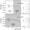 |
Fig. 1. Final chemical profile for two models with MH = 10−4 M⊙ but different effective temperatures. The accretion rate in both cases was 1010 g s−1. |
Final iron surface abundances (in mass) for simulations that turn fingering convection on and off.
Figure 2 displays the temporal evolution of the photosphere’s abundance of iron for an accretion rate of 106 g s−1 at three different effective temperatures. We note that for the hotter models, those with Teff = 8000 K and 10 000 K, the abundance of iron reaches a stationary state well before the end of the simulation, which was set after 14 000 yr of continuous accretion2. However, at the lowest effective temperature, much more time is required to reach the stationary state (about 200 000 yr)3. This is an expected behavior since as the CZ becomes more massive as cooling proceeds, more time is needed to achieve the final (stationary) state. We note that all of our simulations have been extended in order to reach a final state as close as possible to a stationary situation.
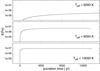 |
Fig. 2. Temporal evolution of the abundance (in mass) of iron for a continuous accretion rate of 106 g s−1 for white dwarf models with a hydrogen content of 10−4 M⊙ at three selected effective temperatures. |
Figure 3 reveals another feature of our simulations, namely the contrast between the time required for the heavy surface elements to reach the stationary state and the evolution of the FCZ. Indeed, while the abundance of iron, as well as that of the other heavy elements accreted (not shown), rapidly reaches a stationary state, the bottom of the FCZ continues moving to deeper layers during white dwarf evolution. This is in contrast with the situation shown in Fig. 4 for the case of a smaller H envelope. Here, the inward advance of the bottom of the FCZ is halted by the H-He transition, where the inverse μ-gradient produced by the accretion is counteracted by the strong chemical gradient at the H-He interface. We note that in this case the evolution of the iron abundance is the same as that shown in Fig. 3 (i.e., the stationary state is reached in a short time).
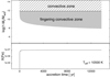 |
Fig. 3. Evolution of a model with MH = 10−4 M⊙. Upper panel: time evolution of the CZ and the FCZ during the accretion period for a model with Teff = 10 500 K and accretion rate of 106 g s−1. Bottom panel: evolution of the iron abundance (in mass) at the surface. |
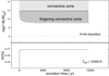 |
Fig. 4. Same as Fig. 3 but for a model with MH = 10−6 M⊙. A dotted horizontal line shows the depth where hydrogen abundance by mass falls below 0.5. |
The impact of a thinner FCZ on the accumulation of heavy elements on the surface increases when the H-He transition is closer to the photosphere of the star. Figure 5 illustrates how thin the FCZ becomes when the hydrogen mass in the envelope is reduced to 10−10 M⊙. In this case the bottom of the CZ penetrates more into the He-rich layers, lowering the contrast between the molecular weights inside the CZ and below. Because of the effect of the stabilizing μ-gradient produced by the increasing helium abundance as we go deeper, fingering convection barely shows up. Therefore, the expected presence of even a small amount of convective overshoot is likely to completely dominate such a small FCZ. The extension of the FCZ also depends on the accretion rate: the higher the accretion rate, the wider the FCZ (not shown in the figure). In the case shown in Fig. 5, the abundance of iron increases by 15% with respect to the cases with a larger hydrogen envelope. This increase is not at all obvious in Fig. 5 but is more evident for higher accretion rates. Figure 6 shows the dependence of the final iron abundances with the amount of hydrogen present in the envelope for three different accretion rates. The maximum difference with respect to the case with a larger hydrogen envelope, an increase of 233%, happens for an accretion rate of 1010 g s−1. In the intermediate case (108 g s−1) the abundance increase is 69%. Other simulations show a much higher accumulation of heavy elements when the FCZ becomes thin.
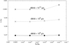 |
Fig. 6. Final abundances (in mass) of iron for envelopes of different amounts of hydrogen and different accretion rates. |
Models with a larger content of hydrogen have the H-He transition deeper, and that may cause this region to be unreachable for the FCZ. In fact, all our simulations that use models with MH = 10−4 M⊙ show that the bottom of the FCZ does not reach the H-He transition layers. Thus, the FCZ finds no obstacle that would prevent it from advancing deeper as the simulation continues, although it slows down its pace as it penetrates into layers of increasing density. In contrast, the bottom of the CZ (when the model has one) always remains at the same depth. Since the extension of the CZ depends on the effective temperature, the level of accumulation of heavy elements on the surface will also depend on this parameter. Cooler models, with larger CZs, rapidly spread the accreted material into this larger region, producing less contamination of the surface than in hotter white dwarfs. The evolution of the FCZ is faster for higher accretion rates; it also goes deeper, carrying the heavy material farther inside the star.
Figure 7 shows the chemical profile at the end of the simulation for a model with MH = 10−4 M⊙, Teff = 10 000 K, and the maximum accretion rate (1012 g s−1). The FCZ extends through a large region of the star (in a logarithmic scale in mass) but is still far from reaching the He-rich layers. Accreted heavy elements are homogeneously distributed throughout the CZ but are less and less abundant as we advance deeper through the FCZ. The turbulence associated with the fingering convective instability is maximum near the bottom of the CZ and diminishes downward, tending gradually to zero. In our 1D computations, there is a somewhat sharp step in turbulence between dynamical CZs and FCZs, which would be smoother if 3D simulations of convection were taken into account (Freytag et al. 1996; Kupka et al. 2018; Cunningham et al. 2019). We did not add any 1D parametrization of overshoot or penetrative convection. A rapidly decreasing extra mixing below the CZ would smoothen the local μ-gradient at the beginning of the simulations. Fingering convection would rapidly take over, leading to similar final results. Detailed computations with various parameterizations of the bottom of the CZs can be undertaken in the future.
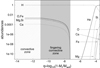 |
Fig. 7. Chemical profile of the final configuration of a model with 10−4 M⊙ of hydrogen, Teff = 10 000 K, and an accretion rate of 1012 g s−1. |
In the case of thinner envelopes, the chemical evolution of accreting white dwarfs is quite different from the MH = 10−4 M⊙ case described before4. The main reason for such a difference is that now the turbulence from the upper layers is able to reach the H-He transition zone, something that does not happen for thicker envelopes.
We can start by describing our results for models with MH = 10−6 M⊙. For such a thin envelope, the FCZ that develops below the CZ expands until it penetrates the transition zone, where He becomes more abundant5. This encounter prevents the FCZ from going deeper, as it is stabilized by the normal μ-gradient due to the increasing amount of He. Thus, the heavy elements accumulated in the FCZ continue to progress farther down by diffusion in a radiative medium, something that never happened in our previously described simulations of models with thicker envelopes, since the presence of heavy elements in a H-rich medium always triggered the fingering convection instability. Figure 8 shows such a situation for a model of Teff = 10 500 K and an accretion rate of 106 g s−1. We expanded the abundance range to include very low values in order to show the contact between the bottom of the FCZ and the He tail, which stops the instability. We also note the dredge-up of He by the FCZ, which leads to the contamination of the surface by a very small amount in this case. As can be seen from Fig. 8, the FCZ stops where the He/H abundance ratio reaches approximately 10−15. The consecutive dredge-up of He would lead to an undetectable He abundance of 10−18.87 in the photosphere (see Table A.1).
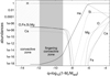 |
Fig. 8. Chemical profile of the final configuration of a model with 10−6 M⊙ of hydrogen, Teff = 10 500 K, and an accretion rate of 106 g s−1. |
Larger He contamination is expected in the case of larger accretion rates (see Fig. 9). In this case, the FCZ is able to further penetrate the H-He transition region, with as a consequence a larger He enrichment of the outer layers. One can see from Fig. 9 that for an accretion rate of 1012 g s−1, the FCZ stops where the He/H abundance ratio reaches approximately 10−4. In this case, our simulation was interrupted before the steady state for the photospheric He abundance could be reached. The achieved lower limit for the abundance of He in the photosphere is 10−6.09 (see Table A.1). The photospheric He abundance depends on both the hydrogen mass fraction and the accretion rate. In the cases where the hydrogen mass fraction could be independently derived and the accretion rate estimated from the observed heavy elements abundances, it should be possible to distinguish whether the photospheric helium has been accreted or dredged up.
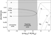 |
Fig. 9. Same as Fig. 8 but for a model with 10−6 M⊙ of hydrogen and Teff = 10 500 K but an accretion rate of 1012 g s−1. |
All the simulations with the highest accretion rates show this kind of behavior. Unfortunately, the abundance of He on the surface takes much longer to reach a steady state than the accreted heavy elements, and we had to stop the simulations before that state was reached because of the excessive time required by the computation. We estimate that it takes on the order of 15 000 yr of evolution to finally reach that steady state. Thus, our tabulated abundances of helium are only lower boundaries in most cases.
About 25% of the parameter space covered in this work was previously studied by Bauer & Bildsten (2019) for a log(MH/Mwd) = − 6 model. Table 3 compares their results with ours, as well as those obtained by Koester (2009). In all cases we show the diffusion calculations using the coefficients of Paquette et al. (1986). Some differences in the CZ are apparent, arising from the differences between the mixing length theory used by those works and the Grossman et al. (1993) convection theory implemented here.
Comparison of the results of Koester (2009), Bauer & Bildsten (2019), and this paper for the mass of the surface CZ and diffusion timescales for 40Ca on a 0.6 M⊙ white dwarf.
Models with MH = 10−8 M⊙ share many of the main features of the MH = 10−6 M⊙ case. Dredge-up of helium is much more efficient now, and consequently the contamination of the surface by helium is noticeably higher. The thinnest envelope models (MH = 10−10 M⊙) continue with the same tendency: more helium contamination of the surface and an FCZ advance stopped earlier by the more superficial H-He transition zone.
Figures 10–A.2 show how the surface contamination changes with the accretion rate for models of four different hydrogen envelopes. The details of the abundances at the end of each simulation are summarized in Tables 4–A.3.
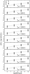 |
Fig. 10. Surface contamination against the accretion rate for models with MH = 10−4 M⊙. The contamination is given in terms of the abundance, expressed in [Z/H] = log n(Z)/n(H). |
Models with MH = 10−4 M⊙.
Figure 11 includes the surface mass fractions for 40Ca obtained by Bauer & Bildsten (2019). Although not strictly the same temperature, we also include their results for Teff = 15 000 K and 20 500 K in our panels for 16 000 K and 20 000 K, respectively. There are some systematic differences for higher temperatures, where we obtain somewhat higher 40Ca abundances than Bauer & Bildsten (2019). A better agreement is found for Teff ≤ 10 000 K, although for Teff = 6000 K we obtain smaller abundances for higher accretion rates. This difference is due to the difficulties in reaching the final steady state in our simulations because of the small timestep needed by our diffusion calculation (in these cases) to fulfill the required precision. Therefore, our results for Teff = 6000 K and high accretion rates should be taken as lower boundaries. Figure 11 also includes for Teff = 11 500 K the steady state abundances for 16O, 24Mg, 28Si, 40Ca, and 56Fe provided by Bauer & Bildsten (2018) using the observed photospheric abundance of pollutants in G29–38. There is a good agreement for the abundances of 24Mg, 28Si, and 56Fe, whereas 16O and 40Ca show higher values (by about Δ[Z/X] = 0.44) in Bauer & Bildsten (2018).
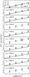 |
Fig. 11. Same as Fig. 10 but for models with MH = 10−6 M⊙. When possible, 40Ca abundances obtained by Bauer & Bildsten (2019) have been added to the corresponding panel (labeled as BB19). For Teff = 11 500 K, gray symbols (inside a box) represent the abundances obtained by Bauer & Bildsten (2018) for 16O, 24Mg, 28Si, 40Ca, and 56Fe using the observed photospheric abundance of pollutants in G29–38. All these isolated points correspond to an accretion rate of 1010 g s−1 but have been shifted a bit from that particular value for the sake of clarity. |
5. Summary and discussion
We have presented a series of numerical simulations concerning the accretion of material produced by the disintegration of small rocky bodies onto DA white dwarfs. These simulations consider the effect of the double-diffusive instability, referred to as fingering convection. This instability is induced by the inverse μ-gradient that results from the accretion of heavy material onto the white dwarf outer layers. Our simulations are aimed at providing realistic estimates of the accretion rates, deduced from the observed heavy element abundances in white dwarf atmospheres, for a large range of effective temperatures, hydrogen-mass fractions, and accretion rates. The results are presented in various graphs and tables in such a way that the accretion rate can easily be deduced from the values of the heavy elements abundances. When fingering convection is properly considered, the resulting accretion rates may be up to several orders of magnitude larger than those estimated when ignoring its effect. For given values of the accretion rate and effective temperature, the accumulation of heavy elements in the white dwarfs’ atmospheres increases for decreasing hydrogen mass fraction since the FCZ becomes thinner when the H/He transition zone is closer to the surface. In the cases of a thin hydrogen mass fraction and high accretion rates, the fingering convection may dredge up some fraction of He from the H/He transition zone (see Tables A.2 and A.3). Such an effect produces DABZ-type white dwarfs. We discuss below the various assumptions that have been adopted in our simulations.
The chemical composition of the accreted material was supposed to be similar to the Earth bulk composition. This is the case for most observed polluted DA white dwarfs (Swan et al. 2019). There is also evidence of other white dwarfs polluted by material with a variety of chemical compositions (Gänsicke et al. 2012; Wilson et al. 2015; Melis & Dufour 2017), including water-rich and hydrated planetesimals (Farihi et al. 2013; Raddi et al. 2015; Hoskin et al. 2020) and volatile-rich planetesimals (Xu et al. 2017). Our simulations are not representative of such cases.
The accreted material was supposed to be mixed through the CZ and through the FCZ. Cunningham et al. (2021) find from their 3D radiation-hydrodynamic simulations that DA white dwarfs with effective temperatures larger than 13 000 K are unable to spread the accreted material horizontally on a timescale shorter than the diffusion timescale. However, these diffusion timescales, estimated at the bottom of the CZ, do not take the additional FCZ into account. By considering fingering convection, diffusion happens deeper in the star and on a timescale that might be significantly longer. The absence of surface abundance variations in polluted DA white dwarfs (Debes & López-Morales 2008; Reach et al. 2009; Wilson et al. 2019) can be explained by (1) horizontal mixing being more efficient than predicted, (2) material being accreted in a generally homogeneous surface distribution, or (3) observations not being sensitive enough to detect variations in abundance. Thus, our assumption of homogeneously mixed pollutants in turbulent zones is consistent with observations.
The mixing induced by the fingering convection was supposed to be a continuous process. The validity of this assumption has been called into question (Koester 2015). However, Brassard & Fontaine (2015) showed that in the case of a DA white dwarf with a hydrogen mass fraction of MH = 10−4 M⊙ and Teff = 11 000 K, the accretion of a C–O mixture at a rate of 9 × 10⁹ g s−1 induces the fingering convection. Bauer & Bildsten (2018, 2019) considered the case of accretion of bulk-Earth composition material and a range of accretion rates from 105 g s−1 to 1012 g s−1. They find that fingering convection develops efficiently for accretion rates above approximately 106 g s−1 (see Fig. 5 in Bauer & Bildsten 2019). Multidimensional simulations accounting for convection and fingering mixing are clearly needed to probe how these two physical processes interact. The agreement between the results of Brassard & Fontaine (2015), Bauer & Bildsten (2018, 2019), and this paper is an indication that fingering convection is properly introduced in our simulations.
We hope that our results, with the figures and tables, will be useful in providing realistic estimates of accretion rates, including the effect of fingering convection, for further studies on evolved planetary systems.
Cunningham et al. (2019) found in their 3D radiation hydrodynamic simulations that a superficial CZ develops at Teff ≈ 18 000 K. Due to numerical stability considerations, particularly related to the treatment of diffusion, 1D evolutionary codes may undergo convergence difficulties when the radially sampling extends too far out into the regions where convection first sets in, thus making it undetectable until the instability penetrates deeper at lower effective temperatures. Thus, it is not surprising that 3D hydrodynamic simulations find convection to start earlier, at higher effective temperatures, than 1D codes.
The end of these simulations was arbitrarily set to 14 000 yr after confirming that a stationary state was reached.
Some simulations took about one week to run and still did not reach a stationary state. In those cases we report a lower value for the particular element in the corresponding table.
Cunningham et al. (2020) found observational evidence that approximately 20% of white dwarfs are expected to have a hydrogen content of −14 < log(MH/Mwd) < − 10 and that approximately 65% are expected to have log(MH/Mwd) > − 10.
We found only two cases where no FCZ was formed. Both simulations correspond to the coolest models (Teff = 6000 K) and to the lower accretion rates (106 and 108 g s−1). Two related factors are responsible for this result. First, the bottom of the CZ deeply penetrates the H-He transition region, reaching a stabilizing μ-gradient due to the increasing abundance of He as we go deeper. Second, the low accretion rate combined with a large CZ (which strongly dilutes the abundance of heavy elements) lowers the difference between the molecular weights at the bottom of the CZ and the region immediately below it. The combination of these factors precludes the formation of the FCZ.
Acknowledgments
We would like to thank an anonymous referee for the helpful comments, and constructive remarks on this manuscript. This work was supported by PICT-2017-0884 from ANPCyT, PIP 112-200801-00940 grant from CONICET, and grant G149 from University of La Plata. This research has made use of NASA Astrophysics Data System. F. C. W., G. V. and S. V. acknowledge financial support from “Programme National de Physique Stellaire (PNPS)” of CNRS/INSU, France.
References
- Alexander, D. R., & Ferguson, J. W. 1994, ApJ, 437, 879 [NASA ADS] [CrossRef] [Google Scholar]
- Allègre, C., Manhès, G., & Lewin, É. 2001, Earth Planet. Sci. Lett., 185, 49 [CrossRef] [Google Scholar]
- Althaus, L. G., & Benvenuto, O. G. 1998, MNRAS, 296, 206 [NASA ADS] [CrossRef] [Google Scholar]
- Althaus, L. G., Serenelli, A. M., Córsico, A. H., & Montgomery, M. H. 2003, A&A, 404, 593 [NASA ADS] [CrossRef] [EDP Sciences] [Google Scholar]
- Althaus, L. G., Serenelli, A. M., Panei, J. A., et al. 2005, A&A, 435, 631 [NASA ADS] [CrossRef] [EDP Sciences] [Google Scholar]
- Althaus, L. G., Camisassa, M. E., Miller Bertolami, M. M., Córsico, A. H., & García-Berro, E. 2015, A&A, 576, A9 [NASA ADS] [CrossRef] [EDP Sciences] [Google Scholar]
- Bauer, E. B., & Bildsten, L. 2018, ApJ, 859, L19 [NASA ADS] [CrossRef] [Google Scholar]
- Bauer, E. B., & Bildsten, L. 2019, ApJ, 872, 96 [NASA ADS] [CrossRef] [Google Scholar]
- Brassard, P., & Fontaine, G. 2015, in 19th European Workshop on White Dwarfs, eds. P. Dufour, P. Bergeron, & G. Fontaine, ASP Conf. Ser., 493, 121 [Google Scholar]
- Brown, J. M., Garaud, P., & Stellmach, S. 2013, ApJ, 768, 34 [NASA ADS] [CrossRef] [Google Scholar]
- Burgers, J. M. 1969, Flow Equations for Composite Gases (New York: Academic Press) [Google Scholar]
- Cassan, A., Kubas, D., Beaulieu, J. P., et al. 2012, Nature, 481, 167 [Google Scholar]
- Chen, E. Y., & Hansen, B. M. S. 2011, MNRAS, 413, 2827 [NASA ADS] [CrossRef] [Google Scholar]
- Christensen-Dalsgaard, J., Silva Aguirre, V., Cassisi, S., et al. 2020, A&A, 635, A165 [NASA ADS] [CrossRef] [EDP Sciences] [Google Scholar]
- Cunningham, T., Tremblay, P.-E., Freytag, B., Ludwig, H.-G., & Koester, D. 2019, MNRAS, 488, 2503 [NASA ADS] [CrossRef] [Google Scholar]
- Cunningham, T., Tremblay, P.-E., Gentile Fusillo, N. P., Hollands, M., & Cukanovaite, E. 2020, MNRAS, 492, 3540 [NASA ADS] [CrossRef] [Google Scholar]
- Cunningham, T., Tremblay, P.-E., Bauer, E. B., et al. 2021, MNRAS, 503, 1646 [NASA ADS] [CrossRef] [Google Scholar]
- Deal, M., Deheuvels, S., Vauclair, G., Vauclair, S., & Wachlin, F. C. 2013, A&A, 557, L12 [NASA ADS] [CrossRef] [EDP Sciences] [Google Scholar]
- Debes, J. H., & López-Morales, M. 2008, ApJ, 677, L43 [NASA ADS] [CrossRef] [Google Scholar]
- Debes, J. H., & Sigurdsson, S. 2002, ApJ, 572, 556 [NASA ADS] [CrossRef] [Google Scholar]
- Debes, J. H., Walsh, K. J., & Stark, C. 2012, ApJ, 747, 148 [NASA ADS] [CrossRef] [Google Scholar]
- Dupuis, J., Fontaine, G., Pelletier, C., & Wesemael, F. 1992, ApJS, 82, 505 [NASA ADS] [CrossRef] [Google Scholar]
- Farihi, J., Gänsicke, B. T., Wyatt, M. C., et al. 2012, MNRAS, 424, 464 [NASA ADS] [CrossRef] [Google Scholar]
- Farihi, J., Gänsicke, B. T., & Koester, D. 2013, Science, 342, 218 [NASA ADS] [CrossRef] [Google Scholar]
- Frewen, S. F. N., & Hansen, B. M. S. 2014, MNRAS, 439, 2442 [NASA ADS] [CrossRef] [Google Scholar]
- Freytag, B., Ludwig, H.-G., & Steffen, M. 1996, A&A, 313, 497 [Google Scholar]
- Freytag, B., Steffen, M., Ludwig, H. G., et al. 2012, J. Comput. Phys., 231, 919 [Google Scholar]
- Gänsicke, B. T., Koester, D., Farihi, J., et al. 2012, MNRAS, 424, 333 [CrossRef] [Google Scholar]
- Garaud, P. 2011, ApJ, 728, L30 [Google Scholar]
- Grossman, S. A., Narayan, R., & Arnett, D. 1993, ApJ, 407, 284 [NASA ADS] [CrossRef] [Google Scholar]
- Hoskin, M. J., Toloza, O., Gänsicke, B. T., et al. 2020, MNRAS, 499, 171 [NASA ADS] [CrossRef] [Google Scholar]
- Iben, I. Jr., Ritossa, C., & García-Berro, E. 1997, ApJ, 489, 772 [NASA ADS] [CrossRef] [Google Scholar]
- Iglesias, C. A., & Rogers, F. J. 1996, ApJ, 464, 943 [NASA ADS] [CrossRef] [Google Scholar]
- Jura, M. 2003, ApJ, 584, L91 [Google Scholar]
- Koester, D. 2009, A&A, 498, 517 [NASA ADS] [CrossRef] [EDP Sciences] [Google Scholar]
- Koester, D. 2015, in 19th European Workshop on White Dwarfs, eds. P. Dufour, P. Bergeron, & G. Fontaine, ASP Conf. Ser., 493, 129 [Google Scholar]
- Koester, D., & Wilken, D. 2006, A&A, 453, 1051 [NASA ADS] [CrossRef] [EDP Sciences] [Google Scholar]
- Koester, D., Gänsicke, B. T., & Farihi, J. 2014, A&A, 566, A34 [NASA ADS] [CrossRef] [EDP Sciences] [Google Scholar]
- Kupka, F., Zaussinger, F., & Montgomery, M. H. 2018, MNRAS, 474, 4660 [NASA ADS] [CrossRef] [Google Scholar]
- Manser, C. J., Gänsicke, B. T., Eggl, S., et al. 2019, Science, 364, 66 [Google Scholar]
- Melis, C., & Dufour, P. 2017, ApJ, 834, 1 [NASA ADS] [Google Scholar]
- Miller Bertolami, M. M. 2016, A&A, 588, A25 [NASA ADS] [CrossRef] [EDP Sciences] [Google Scholar]
- Mustill, A. J., Villaver, E., Veras, D., Bonsor, A., & Wyatt, M. C. 2013, Eur. Phys. J. Web Conf., 47, 06008 [NASA ADS] [CrossRef] [EDP Sciences] [Google Scholar]
- Paquette, C., Pelletier, C., Fontaine, G., & Michaud, G. 1986, ApJS, 61, 177 [Google Scholar]
- Raddi, R., Gänsicke, B. T., Koester, D., et al. 2015, MNRAS, 450, 2083 [NASA ADS] [CrossRef] [Google Scholar]
- Reach, W. T., Lisse, C., von Hippel, T., & Mullally, F. 2009, ApJ, 693, 697 [NASA ADS] [CrossRef] [Google Scholar]
- Renedo, I., Althaus, L. G., Miller Bertolami, M. M., et al. 2010, ApJ, 717, 183 [Google Scholar]
- Salaris, M., Althaus, L. G., & García-Berro, E. 2013, A&A, 555, A96 [NASA ADS] [CrossRef] [EDP Sciences] [Google Scholar]
- Silva Aguirre, V., Christensen-Dalsgaard, J., Cassisi, S., et al. 2020, A&A, 635, A164 [NASA ADS] [CrossRef] [EDP Sciences] [Google Scholar]
- Stancliffe, R. J., Glebbeek, E., Izzard, R. G., & Pols, O. R. 2007, A&A, 464, L57 [NASA ADS] [CrossRef] [EDP Sciences] [Google Scholar]
- Swan, A., Farihi, J., Koester, D., et al. 2019, MNRAS, 490, 202 [NASA ADS] [CrossRef] [Google Scholar]
- Vanderburg, A., Johnson, J. A., Rappaport, S., et al. 2015, Nature, 526, 546 [Google Scholar]
- Van Grootel, V., Dupret, M. A., Fontaine, G., et al. 2012, A&A, 539, A87 [NASA ADS] [CrossRef] [EDP Sciences] [Google Scholar]
- Vauclair, S. 2004, ApJ, 605, 874 [Google Scholar]
- Veras, D. 2016, R. Soc. Open Sci., 3, 150571 [Google Scholar]
- Veras, D., Mustill, A. J., Bonsor, A., & Wyatt, M. C. 2013, MNRAS, 431, 1686 [NASA ADS] [CrossRef] [Google Scholar]
- Veras, D., Jacobson, S. A., & Gänsicke, B. T. 2014a, MNRAS, 445, 2794 [NASA ADS] [CrossRef] [Google Scholar]
- Veras, D., Leinhardt, Z. M., Bonsor, A., & Gänsicke, B. T. 2014b, MNRAS, 445, 2244 [NASA ADS] [CrossRef] [Google Scholar]
- Veras, D., Eggl, S., & Gänsicke, B. T. 2015a, MNRAS, 452, 1945 [NASA ADS] [CrossRef] [Google Scholar]
- Veras, D., Eggl, S., & Gänsicke, B. T. 2015b, MNRAS, 451, 2814 [Google Scholar]
- Veras, D., Leinhardt, Z. M., Eggl, S., & Gänsicke, B. T. 2015c, MNRAS, 451, 3453 [NASA ADS] [CrossRef] [Google Scholar]
- Veras, D., Mustill, A. J., Gänsicke, B. T., et al. 2016, MNRAS, 458, 3942 [Google Scholar]
- Wachlin, F. C., Miller Bertolami, M. M., & Althaus, L. G. 2011, A&A, 533, A139 [NASA ADS] [CrossRef] [EDP Sciences] [Google Scholar]
- Wachlin, F. C., Vauclair, S., & Althaus, L. G. 2014, A&A, 570, A58 [NASA ADS] [CrossRef] [EDP Sciences] [Google Scholar]
- Wachlin, F. C., Vauclair, G., Vauclair, S., & Althaus, L. G. 2017, A&A, 601, A13 [EDP Sciences] [Google Scholar]
- Wilson, D. J., Gänsicke, B. T., Koester, D., et al. 2015, MNRAS, 451, 3237 [NASA ADS] [CrossRef] [Google Scholar]
- Wilson, D. J., Gänsicke, B. T., Koester, D., et al. 2019, MNRAS, 483, 2941 [NASA ADS] [CrossRef] [Google Scholar]
- Xu, S., Jura, M., Koester, D., Klein, B., & Zuckerman, B. 2014, ApJ, 783, 79 [NASA ADS] [CrossRef] [Google Scholar]
- Xu, S., Zuckerman, B., Dufour, P., et al. 2017, ApJ, 836, L7 [Google Scholar]
- Xu, S., Dufour, P., Klein, B., et al. 2019, AJ, 158, 242 [NASA ADS] [CrossRef] [Google Scholar]
- Zemskova, V., Garaud, P., Deal, M., & Vauclair, S. 2014, ApJ, 795, 118 [Google Scholar]
- Zuckerman, B., & Becklin, E. E. 1987, Nature, 330, 138 [NASA ADS] [CrossRef] [Google Scholar]
- Zuckerman, B., Koester, D., Reid, I. N., & Hünsch, M. 2003, ApJ, 596, 477 [Google Scholar]
- Zuckerman, B., Koester, D., Melis, C., Hansen, B. M., & Jura, M. 2007, ApJ, 671, 872 [Google Scholar]
Appendix A: Additional material
Same as Table 4 but for models with MH = 10−6 M⊙.
Same as Table 4 but for models with MH = 10−8 M⊙.
Same as Table 4 but for models with MH = 10−10 M⊙.
All Tables
Final iron surface abundances (in mass) for simulations that turn fingering convection on and off.
Comparison of the results of Koester (2009), Bauer & Bildsten (2019), and this paper for the mass of the surface CZ and diffusion timescales for 40Ca on a 0.6 M⊙ white dwarf.
All Figures
|
Fig. 1. Final chemical profile for two models with MH = 10−4 M⊙ but different effective temperatures. The accretion rate in both cases was 1010 g s−1. |
| In the text | |
|
Fig. 2. Temporal evolution of the abundance (in mass) of iron for a continuous accretion rate of 106 g s−1 for white dwarf models with a hydrogen content of 10−4 M⊙ at three selected effective temperatures. |
| In the text | |
|
Fig. 3. Evolution of a model with MH = 10−4 M⊙. Upper panel: time evolution of the CZ and the FCZ during the accretion period for a model with Teff = 10 500 K and accretion rate of 106 g s−1. Bottom panel: evolution of the iron abundance (in mass) at the surface. |
| In the text | |
|
Fig. 4. Same as Fig. 3 but for a model with MH = 10−6 M⊙. A dotted horizontal line shows the depth where hydrogen abundance by mass falls below 0.5. |
| In the text | |
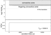 |
Fig. 5. Same as Fig. 4 but for a model with MH = 10−10 M⊙. |
| In the text | |
|
Fig. 6. Final abundances (in mass) of iron for envelopes of different amounts of hydrogen and different accretion rates. |
| In the text | |
|
Fig. 7. Chemical profile of the final configuration of a model with 10−4 M⊙ of hydrogen, Teff = 10 000 K, and an accretion rate of 1012 g s−1. |
| In the text | |
|
Fig. 8. Chemical profile of the final configuration of a model with 10−6 M⊙ of hydrogen, Teff = 10 500 K, and an accretion rate of 106 g s−1. |
| In the text | |
|
Fig. 9. Same as Fig. 8 but for a model with 10−6 M⊙ of hydrogen and Teff = 10 500 K but an accretion rate of 1012 g s−1. |
| In the text | |
|
Fig. 10. Surface contamination against the accretion rate for models with MH = 10−4 M⊙. The contamination is given in terms of the abundance, expressed in [Z/H] = log n(Z)/n(H). |
| In the text | |
|
Fig. 11. Same as Fig. 10 but for models with MH = 10−6 M⊙. When possible, 40Ca abundances obtained by Bauer & Bildsten (2019) have been added to the corresponding panel (labeled as BB19). For Teff = 11 500 K, gray symbols (inside a box) represent the abundances obtained by Bauer & Bildsten (2018) for 16O, 24Mg, 28Si, 40Ca, and 56Fe using the observed photospheric abundance of pollutants in G29–38. All these isolated points correspond to an accretion rate of 1010 g s−1 but have been shifted a bit from that particular value for the sake of clarity. |
| In the text | |
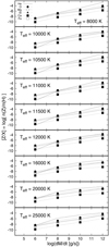 |
Fig. A.1. Same as Fig. 10 but for models with MH = 10−8 M⊙. |
| In the text | |
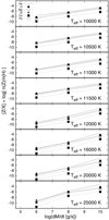 |
Fig. A.2. Same as Fig. 10 but for models with MH = 10−10 M⊙. |
| In the text | |
Current usage metrics show cumulative count of Article Views (full-text article views including HTML views, PDF and ePub downloads, according to the available data) and Abstracts Views on Vision4Press platform.
Data correspond to usage on the plateform after 2015. The current usage metrics is available 48-96 hours after online publication and is updated daily on week days.
Initial download of the metrics may take a while.