| Issue |
A&A
Volume 660, April 2022
|
|
|---|---|---|
| Article Number | A101 | |
| Number of page(s) | 15 | |
| Section | Stellar structure and evolution | |
| DOI | https://doi.org/10.1051/0004-6361/202141399 | |
| Published online | 20 April 2022 | |
Binary orbital evolution driven by a circumbinary disc
Institut für Astronomie und Astrophysik, Universität Tübingen, Auf der Morgenstelle 10, 72076 Germany
e-mail: This email address is being protected from spambots. You need JavaScript enabled to view it.
Received:
27
May
2021
Accepted:
11
February
2022
Abstract
The question whether the interaction of a circumbinary disc with the central binary system leads to a shrinking or to an expansion of the binary orbit has attracted considerable interest as it impacts the evolution of binary black holes and stellar binary stars in their formation phase. We performed two-dimensional hydrodynamical simulations of circumbinary discs for a large parameter set of disc viscosities and thicknesses and for two different binary mass ratios for binaries on circular orbits. We measured the net angular momentum and mass transfer between disc and binary system, and evaluated the normalised specific angular momentum accretion, js. This was compared to the theoretical, critical specific angular momentum change js,crit that separates contracting from expanding cases, which depends on the binary mass ratio and on the relative accretion onto the two stars. Using finite and infinite disc models, we show that the inferred binary evolution is very similar for both setups, and we confirm that js can be measured accurately with cylindrical simulations that do not include the central binary. However, to obtain the relative accretion onto the stars for non-equal mass binaries, simulations that cover the whole domain including the binary are required. We find that for thick discs with aspect ratio h = 0.1, the binaries expand for all viscosities, while discs with h = 0.05 lead to an expansion only for higher viscosities with α exceeding ∼0.005. Overall, the regime of binary expansion extends to a much wider parameter space than previously anticipated, but for thin, low-viscosity discs, the orbits shrink.
Key words: binaries: general / accretion, accretion disks
Deceased.
© ESO 2022
1. Introduction
Circumbinary (CB) discs orbiting two gravitating objects exist over a wide range of spatial scales, starting from spectroscopic binary stars, then to large binary systems like GG Tau, and finally all the way to galactic discs around binary black holes. The binary star and the disc resemble a coupled system that exchanges mass and angular momentum between its components leading possibly to a secular evolution of the binary’s orbit, i.e. changes in its semi-major axis and eccentricity. Due its gravitational action the binary transfers angular momentum to the disc. As a consequence the disc recedes from the binary opening a central cavity, while the binary reacts with a shrinkage orbit accompanied by an increase in its eccentricity (Artymowicz et al. 1991). In the context of black holes such a disc induced orbital evolution was already suggested by Begelman et al. (1980) to overcome the so called ‘final parsec problem’ (Milosavljević & Merritt 2003), i.e. the necessary contraction of the orbit such that gravitational wave emission can set in. In the context of binary star formation a CB-disc will be formed that determines the binary orbital evolution similarly.
Given the binary’s gravitational torque acting on the CB-disc and its own angular momentum loss, it was always assumed that the binary can only react with a shrinkage of the orbit. This point of view was questioned by Miranda et al. (2017), who argued that for a certain binary parameter the mass accretion and hence the accreted angular momentum onto the central binary can counterbalance and even overcome the disc torques, leading to an expansion of the orbit. This has led to an increased activity in studies of the still controversial issue of binary orbit evolution in more detail using various numerical approaches.
In their simulations, Miranda et al. (2017) used a grid code operating in cylindrical coordinates, where the binary stars orbited inside of the computational domain. Their evolution was calculated by monitoring the mass and angular momentum balance of the surrounding disc. Concerns about the impact of the inner radius of the grid on the outcome were resolved by simulations that covered the whole domain, including the stars. Using a moving mesh code, Muñoz et al. (2019) presented simulations that covered the whole domain and clearly demonstrated that the orbits of binary stars can indeed expand due to the action of a CB disc. This result was confirmed by Moody et al. (2019) using a Cartesian grid. The topic of binary evolution was treated subsequently by different groups (e.g. Muñoz et al. 2020; Duffell et al. 2020; Tiede et al. 2020; Heath & Nixon 2020; Zrake et al. 2021) using different numerical approaches.
The first works (Miranda et al. 2017; Muñoz et al. 2019; Moody et al. 2019) focused primarily on equal-mass binaries surrounded by discs with high viscosity (α = 0.1) and larger thickness (H/r = 0.1) because they reach a quasi-stationary state earlier and are easier to simulate. Taking into account the disc backreaction on the binary, Muñoz et al. (2019) showed that initially, circular binaries remain circular during the evolution. Later, Muñoz et al. (2020) performed a larger parameter survey in which they varied the viscous α parameter from 0.01 to 0.1 and the binary star mass ratio M2/M1 from 0.1 to 1.0. They found that binaries with a higher mass ratio (M2/M1 > 0.3) expand independently of the α-value.
The quoted studies agree that for an equal-mass binary system inside a thick disc with H/r ∼ 0.1 and high viscosity, the added angular momentum of the disc is sufficient to allow for an expanding binary orbit. However, Tiede et al. (2020) applied a constant kinematic viscosity, varied the disc thickness, and found that for thinner discs with H/r ≲ 5%, the trend reverses and the binary orbit shrinks again. According to Tiede et al. (2020), the reason for the change of this behaviour lies in the fact that in thinner discs, the cavity is deeper and more material remains near the cavity walls. This exerts a negative torque on the binary.
In general, disc parameters such as scale height and viscosity influence the shape and size of the eccentric inner disc cavity (Thun et al. 2017; Thun & Kley 2018; Hirsh et al. 2020; Penzlin et al. 2021), which in turn impacts the transfer of angular momentum between disc and binary. It is still an open question how the binary orbit will evolve for ranges of physical disc parameter towards low viscosity and disc heights. In this paper we present our results of a wider parameter study. In particular, we are interested in thin discs resembling a protoplanetary environment.
Using two binary mass ratios, we compute the evolution of a CB disc, vary the viscosity and aspect ratio independently, and calculate the orbital evolution of the binary. We present models using an α-type disc viscosity and constant viscosity models. Our study is restricted to circular binaries to reduce the changing orbit parameters to the semi-major axis and make long model runs for low viscosities feasible.
We confirm the statement made by Miranda et al. (2017) that the change in semi-major axis for binaries can be accurately obtained from simulations using a cylindrical grid that surrounds the binary if all the relevant fluxes across the boundaries are measured and for a known mass accretion ratio of the stars. Using infinite and finite disc profiles, we show that the inferred binary evolution is very similar for both setups (see also Muñoz et al. 2020). We expand the parameter range to thinner and less viscous discs that are relevant for protoplanetary scenarios, and determine the transition between expanding and shrinking binary orbits. To validate our results, we use two grid codes that employ different numerical algorithms, RH2D (Kley 1989, 1999) and PLUTO (Mignone et al. 2007; Thun et al. 2017). To directly estimate the mass accretion onto the individual stars, we used RH2D on a Cartesian grid and additionally used smoothed particle hydrodynamics (SPH) simulations (Schäfer et al. 2016) (see Appendix B).
In Sect. 2 we discuss the angular momentum evolution of the disc and binary from a theoretical standpoint and define a critical specific angular momentum accretion rate that separates inspirals from expansions. We present our physical and numerical setup for the two simulation codes in Sect. 3 and display in Sect. 4 the results of the simulations for one standard model. Section 5 gives an overview of the results for our parameter sets in viscosity, scale height, and binary mass ratio. Finally, we discuss and summarise our findings in Sect. 6.
2. Angular momentum evolution of the disc and binary
Before presenting our numerical results, we briefly discuss the orbital evolution of the central binary from a theoretical standpoint. Similar considerations were presented for example by Muñoz et al. (2019) and Dittmann & Ryan (2021). For a binary with total mass Mb, semi-major axis a, and eccentricity e, the orbital angular momentum is given by
![Mathematical equation: $$ \begin{aligned} J_{\rm b} = \mu _{\rm b} \left[GM_{\rm b} a (1 - e^2)\right]^{1/2}, \end{aligned} $$](/articles/aa/full_html/2022/04/aa41399-21/aa41399-21-eq1.gif) (1)
(1)
where
 (2)
(2)
is the reduced mass and q = M2/M1 is the mass ratio of the binary star with M2 ≤ M1. The time evolution of the angular momentum involves changes of the four quantities Mb(t),q(t),a(t), and e(t), which in turn requires knowledge about four parameters: the changes in total mass, orbital angular momentum, and momentum, and knowledge about the distribution of the accreted mass and momentum amongst the two stars. These distributions can be calculated in simulations that include the binaries and flows onto the binaries in the domain with high resolution, as was done for example in Muñoz et al. (2020) for thick discs. For long runs with low viscosity and thin discs, a domain including the binary is currently not feasible.
We assume e = 0 from now on throughout. By restricting our study to circular binaries with maximum angular momentum for given masses, any addition of angular momentum will not increase the eccentricity, but rather lead to an expansion of the orbit, which remains circular. This is supported by simulations of Muñoz et al. (2019), who reported only a very small increase in binary eccentricity in their simulations. Hence, we do not consider any change in binary eccentricity and set ė = 0. Taking the time derivative of Eq. (1) for circular binaries yields
 (3)
(3)
where the change in mass ratio,  in terms of the mass changes of the individual stars is given by
 (4)
(4)
The change in binary mass is directly given by the mass accretion rate from the disc, that is, the material that is advected from the disc onto the stars, Ṁb = Ṁadv, but for the change in angular momentum, there are two contributions, first the accreted angular momentum from disc,  , which accompanies the mass flux, and secondly, the gravitational torque exerted by the disc on the binary,
  . In principle, there could also be a viscous angular momentum flux across the inner boundary (positive or negative), but this turned out to be very small in our simulations and is neglected here. The angular momentum change of the binary can either go into the orbit and/or into the spins of the individual stars. Here, we assume that the latter contribution is overall small, as shown in Muñoz et al. (2019), and consider only the change in the binary orbit.
In our typical long-term simulations, the stars are not within the computational domain, hence in order to account for the a priori unknown distribution of mass amongst the two stars, we introduce the factor f. It denotes the mass distribution between the individual stars and is defined by
 (5)
(5)
which means that the secondary receives f times as much mass as the primary. Then we find with Eq. (4)
 (6)
(6)
To rewrite Eq. (3) in terms of the change in semi-major axis, as we use  , and define the (normalised) specific angular momentum transfer js, to the binary as
 (7)
(7)
The change in semi-major axis of the binary can then be written as
![Mathematical equation: $$ \begin{aligned} \frac{\dot{a}}{a} = \frac{\dot{M}_{\rm adv}}{M_{\rm b}} \left[2\, j_{\rm s} \frac{(q+1)^2}{q} - 3 - 2 \frac{1-q}{1+f} \, \left(\frac{f}{q}-1\right)\right]. \end{aligned} $$](/articles/aa/full_html/2022/04/aa41399-21/aa41399-21-eq12.gif) (8)
(8)
This equation is equivalent to Eq. (9) in Muñoz et al. (2020), where their angular momentum accretion eigenvalue is given by l0 = jsa2Ωb and their preferential accretion ratio is η ≡ Ṁ2/Ṁb = f/(1+f). A similar expression was given by Dittmann & Ryan (2021). To find the critical js at which the orbit changes from contracting to expanding, we set ȧ = 0 and obtain
 (9)
(9)
If the specific angular momentum transfer is larger than js,crit, the binary orbit expands, while it contracts for js smaller than the critical value. For equal-mass binaries with q = 1, only the first term remains and equals 3/8, identical to the value found by Miranda et al. (2017) that was later used by Tiede et al. (2020). In Fig. 1 the critical values of the angular momentum transfer, js,crit, are shown as a function of the mass ratio, q, for selected sample values for the mass accretion ratio, f, of the stars. All values of js,crit are between 0 and 1 for any value of q or f. As discussed above, for q → 1, all curves converge to js,crit = 3/8. When both stars accrete the same mass, f = 1, the critical js,crit lies always above 3/8. It becomes maximal if the secondary star were to accrete all mass, f → ∞. In the following we present the results of our hydrodynamical simulations to analyse for which binary and disc parameter the specific angular momentum accretion is larger than js,crit and thereby sufficient to lead to an expanding binary orbit.
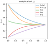 |
Fig. 1. Critical angular momentum transfer to the binary as a function of the binary mass ratio for different values of the accretion factor; see Eq. (9). If the binary receives angular momentum at a rate higher than js, crit, then its orbit expands. We display five different values for the factor f that enclose all cases between the two limiting cases of f = 0 (accretion only on the primary) and f → ∞ (accretion only on the secondary). |
3. Modelling
In this section we first describe our physical setup, then the numerical methods and boundary conditions, and finally the measuring procedure of the mass and angular momentum balance.
3.1. Physical setup
We restricted ourselves to infinitesimally thin two-dimensional (2D) discs that orbit a central binary. The plane of the disc and the binary are coplanar. The system is modelled using polar coordinates with the origin at the centre of mass (COM) of the binary star. For the simulations we kept the binary orbit fixed and the disc was not self-gravitating. To allow for a scale-free setup, we adopted a locally isothermal equation of state with respect to the binary COM. The disc was not flared but had a constant disc aspect ratio h = H/r, where H is the pressure scale height of the disc at distance r. For the viscosity, we assumed the classic alpha-ansatz and write for the kinematic viscosity coefficient ν = αcs H, where cs is the isothermal sound speed of the gas.
For the initial setup of our problem, we followed Muñoz et al. (2020) and used a finite extent of the initial density distribution, which has the shape of a circular gas torus around the binary. For this purpose, we defined the two radii rin and rout, and the two functions
![Mathematical equation: $$ \begin{aligned} g_{\rm in}(r) = \frac{1}{1 + \exp {[- (r - r_{\rm in})/(0.1 \, r_{\rm in})]}} \end{aligned} $$](/articles/aa/full_html/2022/04/aa41399-21/aa41399-21-eq14.gif) (10)
(10)
and
![Mathematical equation: $$ \begin{aligned} g_{\rm out}(r) = \frac{1}{1 + \exp {[r - r_{\rm out}]}}\cdot \end{aligned} $$](/articles/aa/full_html/2022/04/aa41399-21/aa41399-21-eq15.gif) (11)
(11)
The initial density is then given by
![Mathematical equation: $$ \begin{aligned} \Sigma _0(r) = \Sigma _{\rm base}(r) \times \left[1 - \frac{0.7}{\sqrt{r}}\right] \times g_{\rm in}(r) \times g_{\rm out}(r). \end{aligned} $$](/articles/aa/full_html/2022/04/aa41399-21/aa41399-21-eq16.gif) (12)
(12)
Here, Σbase(r) denotes a basic power-law profile for the density, for which we used Σbase(r)∝r−1/2 throughout. The constants were chosen such that shapes similar to Muñoz et al. (2020) can be constructed. These cut-off functions create a smooth transition to a low density beyond rin and rout. Varying these can be a useful start from conditions closer to the convergent state. An example of such an initial Σ-profile is displayed below in Fig. 2 for our standard model.
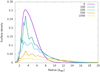 |
Fig. 2. Azimuthally averaged surface density for the standard model (q = 0.5, h = 0.1, α = 0.1) at five different times, quoted in binary orbits. |
To have a well-defined test case, we defined a standard model that has the following parameters: For the binary, we chose q = M2/M1 = 0.5, and for the disc, we adopted α = 0.1 and h = H/r = 0.1 (like Muñoz et al. 2019). Here, the high viscosity and disc thickness allow a fast evolution of the disc, and disc matter is accreted rapidly onto the binary and spreads outwards.
The parameters of the standard model and for the initial surface density are summarised in Table 1. In a detailed parameter study, we studied the effect of varying the viscosity α and aspect ratio h for two values of the binary mass ratio q.
Summary of the physical parameters for the standard model.
3.2. Numerics
For the main part of this paper, we performed numerical simulations over very long timescales in order to cover discs with alpha-viscosities down to 10−3. To allow for a reasonable computational time, the binary stars are not included in the domain. In Appendix B.1 we present an example of a completely covered inner domain for the standard model to the derive the accretion ratio f.
We used two grid-based codes operating on a cylindrical grid stretching from rmin = a to rmax = 40 a with 684 logarithmically spaced radial grid cells and 584 azimuthal cells. Following our previous study (Thun & Kley 2018), the value rmin = a captures the essential dynamics for discs with a significant inner cavity, and we used this value for our parameter study. We show in Sect. 4.3 how the choice of rmin might affect our measured accretion of mass, angular momentum, and js. The outer radius has to be chosen large enough such that it does not impact the disc evolution for large and eccentric cavities. Here, we found rmax = 40 a sufficient. The simulations were carried out in dimensionless units, where the unit of length is the binary separation a, the gravitational constant is G = 1, the binary mass is M = 1, and the binary orbital angular velocity is Ωb = 1.
An important ingredient of grid-based simulations is the necessity of a density floor to prevent negative densities and pressures. For the standard case with its high aspect ratio and high viscosity, the inner region close to the stars is never entirely empty, such that a floor density of ≈10−6 of the initial maximum density is sufficient. However, for the parameter studies with very small h and α, the cavities around the binary become very deep, and much lower floor values ≈10−10 − 10−8 are required in order to follow the very weak mass and angular momentum accretion onto the binary.
In order to validate our results, we first calculated the standard model using two grid codes with different numerics, RH2D (Kley 1989) and PLUTO (Mignone et al. 2007). We describe the details of the codes and comparison runs in Appendix A.
3.3. Boundary conditions
The cylindrical grid simulations conserve global angular momentum, at least within the active domain. In our models, the inner boundary (at rmin) is open to angular momentum and mass flow towards the star. We used an inner radial boundary condition of ∂Σ/∂r = 0 for the density, ∂Ω/∂r = 0 for the azimuthal velocity, and a diode-type radial infall with vr, ghost = min(vr, min, 0). The zero gradient condition for the angular velocity implies a vanishing torque at the inner boundary, at least for circular flows, and ensures that the disc is not artificially torqued from the inside. We tested other conditions for Ω(rmin), such as zero gradients of the angular momentum, but found no differences in the disc evolution. At the outer boundary, we used reflecting conditions where the radial velocity was set to zero at the outer boundary, vr, max = 0. For the azimuthal velocity, we assumed circular Keplerian velocity around the binary COM. While the outer boundary is closed to mass flow, angular momentum is nevertheless transmitted through rmax through viscous torques. This was monitored during the evolution. Additional models resembling an infinite disc setup are presented in Sect. 5.4.
3.4. Measuring the angular momentum and mass balance
To calculate the orbital evolution of the binary, we need to monitor the mass and angular momentum accretion from the disc. Even though these are losses with respect to the disc, we considered the gain with respect to the binary star and took them as positive quantities, denoting them as Ṁadv and  . The subscript ‘adv’ denotes advection (transport) of the quantities across the inner radius of the disc. For the mass flux, this transport is solely advective and is given by
 (13)
(13)
where vr is the radial velocity of the gas, which can only be negative (or zero) for the boundary condition we used, that is, vr(rmin)≤0. For the angular momentum accretion, the advective transport across the inner boundary reads
 (14)
(14)
We evaluated the angular momentum and mass flow rate through the inner boundary, typically at rmin = a. As a consistency test, we also measured the flow at different inner radii in the same model (r = [1.25, 1.5, 2] a). For the equilibrium state, we find the same values, as expected. However, for even smaller inner evaluation radii, the circum-secondary disc can interfere with the calculated advection, depending on the mass ratio. More details on smaller rmin models are shown below in Sect. 4.3. The second change in the binary angular momentum is due the gravitational torque of the disc,
 (15)
(15)
While the advective transport is always positive, this last contribution can take both signs. While the quantities Ṁadv and  are sufficient to evaluate the orbital evolution for circular binaries, it is very useful to have a simple alternative measuring instrument. This was accomplished by simply monitoring the total disc mass, Mdisc, and angular momentum Jdisc within the computational domain. As the outer boundary at rmax is closed, −Ṁdisc = Ṁadv. For the angular momentum, there is an additional viscous loss channel through the outer boundary, given by
 (16)
(16)
with the viscous stress tensor
 (17)
(17)
Written in this way, the sign of  denotes either gains (> 0) or losses from the disc (< 0). Thus the angular momentum can be compared using
  . This monitoring of the global disc properties throughout the simulations allows a very useful consistency check on overall mass and angular momentum conservation of the numerics.
4. Standard model
In this section we present our results for the standard model with the parameters listed in Table 1. First, we provide a general overview of the main disc physics, followed by a discussion of the choice of the inner radius of the domain, rmin, and then the expected binary evolution.
4.1. Disc structure
Most of the results quoted in this subsection were obtained with the RH2D code, unless otherwise stated. Given the inner and outer radii, rin = 2.5 and rout = 6 for the standard model, an initial density setup similar to Muñoz et al. (2020) was generated, as shown in Fig. 2. The density has its maximum near r = 3.5 a and smoothly decreases inwards and outwards. The initial and subsequent evolution of the azimuthally averaged surface density, displayed at five different snapshots in Fig. 2, shows a radial spreading of this initial ring-like density, while the maximum of Σ(r) always remains close to the initial one. The evolution is very fast for this setup. At t = 200 Tbin the density maximum has already dropped by about a factor of three, and the disc has lost about 20% of its initial mass through the inner boundary. To give an impression of the dynamical features of the disc flow in the vicinity of the binary, we present in Fig. 3 the 2D density distribution after a simulated time of 500 Tbin.
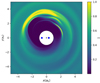 |
Fig. 3. 2D surface density distribution at 500 Tbin for the standard setup. The black cross marks the binary barycenter, and the region within r = 1 abin is not part of the computational domain. |
To have an indicator of the size and distortion of the inner cavity as the simulations evolved, we fit approximate ellipses to its shape using the procedure described in Thun et al. (2017). The result for the semi-major axis acav and eccentricity ecav of the cavity is displayed in Fig. 4 for the two different codes we used in our main study. After a brief initial growth phase that lasted for about 200−300 binary orbits, the cavity size reached a maximum radial extent of acav ∼ 2.25 a and a moderate eccentricity of ecav ∼ 0.18. The shape of the cavity (for these disc parameters) was only an approximate ellipse, such that the automatic fitting routine (see Thun et al. 2017) may be misguided by local density maxima peaks, as seen in Fig. 3. As a consequence, the values vary strongly, as indicated by the grey shaded points. This issue is significantly reduced for simulations with lower viscosities as the density inside the spirals is reduced and the peak density is clearly located at the apocentre of the inner disc; see also Penzlin et al. (2021). The results for the two grid codes agree reasonably well. Differences can be due the fact that in RH2D, the results are computed automatically on the fly while the simulations are running, whereas for PLUTO, they are obtained in a post-processing step from different snapshots, here once every Tbin. In the following, we display smoothed results, here averaged over 10 Tbin.
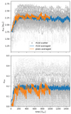 |
Fig. 4. Approximated cavity size and eccentricity for the standard model. The curves denoted ‘averaged’ denote the sliding averages over ten orbits for three different codes. The grey dots show the instantaneously estimated values. |
4.2. Mass and angular momentum balance
During the computation, we monitored the global mass and angular momentum (AM), and the fluxes across the outer and inner boundary as well. To obtain an idea of the importance of the individual contributions, we display the individual loss and gain channels in Fig. 5, labelled (1) to (3). In addition, we display the sum of all three contributions and show that it exactly matches the rate of change in mass and AM as calculated from the time evolution of the global disc values, denoted by ‘derivative’ in the plot. This shows that our measurements are fully consistent and that we can accurately track all loss and gain channels of mass and AM. Figure 5 shows that the torques from the binary create a positive input of AM to the disc (blue curve), while the loss through the inner boundary represents a loss term (red curve). The sum (in green) shows that during a short initial phase (≈40 Tbin), the disc gains more angular momentum from the binary than it loses. After this, the losses dominate, and the disc loses angular momentum to the binary. The loss of angular momentum through the outer boundary (purple curve) is negligible for the first 1000 Tbin. However, it begins to be the main loss channel after about 2300 Tbin when the disc has spread so much that  .
.
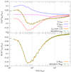 |
Fig. 5. Loss and gain channels of mass and angular momentum, Ṁ and |


The results for the mass and AM fluxes displayed in Fig. 5 were then used to calculate the specific angular momentum transfer, js, to the binary according to Eq. (7). The outcome is displayed in Fig. 6, where we plot js as a function of time for the standard model. Initially, js rose steeply until it reached a maximum at t ≈ 300 Tbin, after which it slowly decreased to reach an equilibrium value after about 1000 Tbin of about js = 0.84. This equilibrium of js was obtained even though the overall disc density, mass, and AM were still evolving in time and no steady state was formally reached. The reason lies in the fact that the inner disc region had reached dynamical equilibrium, as Fig. 4 already indicated. The angular momentum flux js represents an eigenvalue of the disc, as shown already by Miranda et al. (2017) and Muñoz et al. (2019).
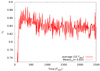 |
Fig. 6. Specific angular momentum transfer, js, onto the binary for the standard model. The curve represents a sliding average over ten orbits, and the grey line shows the average over the last 1000 orbits. |
Using the measured js = 0.84 and the quoted critical values in Fig. 1, we can argue that this leads to an expansion of the binary orbit for a mass ratio q = 0.5 and the chosen disc parameter because js = 0.84 > js,crit for all possible accretion ratios f. This statement about the orbital evolution of a circular binary is possible even though we do not include the binary explicitly in the computational domain, because all the mass and angular momentum that crosses the inner boundary has to be accreted by the binary. A necessary requirement is the establishment of a quasi-stationary state at least in the inner regions of the disc, which can be checked for example by monitoring properties such as acav, ecav, and js directly. The value of rmin must be chosen small enough to include the relevant disc dynamics and the diode inner boundary condition does not impact the results. In the next section, we show that the measured value of js does not depend on the exact location of the inner boundary once rmin ≲ abin.
4.3. Varying the inner radius of the grid
The determination of the angular momentum flux js depends on the details of the disc structure around the binary. It is known from previous studies (Thun et al. 2017) that this can depend on the location of the inner grid radius, rmin. In order to validate our results and determine the numerical impact of this choice, we performed additional computations using different values rmin = 1.25, 1.1, 1.0, 0.7, and 0.5. For this study, we adapted the number of radial grid cells such that we always had the same spatial resolution in the overlapping region. In Fig. 7 we display the azimuthally averaged surface density at 500 binary orbits for the standard model for the different rmin, now for the whole spatial domain. In the outer disc region, beyond roughly 4 a, the density distributions are very similar for all rmin ≤ 1.0 a. They all reach similar maximum densities, but the two models with larger rmin (1.1, 1.25) have substantially lower peak values and are much smoother. This means that spirals in the disc are reduced, which causes perturbations in the density profile. The rmin = 1.25 model does not display any spirals and is therefore dynamically very different. For the model with the smallest rmin = 0.5, there is a pronounced maximum in the density distribution at the location of the secondary star because material is collecting in its potential minimum. For the overall size and shape of the cavity, that is, its eccentricity and semi-major axis, we also find good agreement for the smaller rmin and deviations for the two higher values.
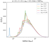 |
Fig. 7. Azimuthally averaged density for five different inner grid radii rmin after 500 binary orbits for simulations using the PLUTO code. |
A similar result is obtained for the important mass and AM balance of the disc. In the top panels of Fig. 8 we display the time evolution of the disc mass and AM loss and gain rates. For the models with rmin ≲ 1, they are identical during the whole evolution, but for larger inner boundaries, the accretion rates increase in an unphysical way. For the specific angular momentum accretion js onto the binary, displayed in bottom panel of Fig. 8, the results are very similar as well for the three models with the smaller rmin. Hence, for sufficiently small rmin, the evolution is indeed solely given by the physical parameter of the system. We therefore conclude that rmin = 1.0 is sufficient even for the highest values of viscosity and aspect ratio, for which the inner region around the two stars is not entirely empty. Hence, we adopt this value for our subsequent models and the parameter study as it represents a good compromise between physical accuracy and computational speed.
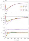 |
Fig. 8. Evolution of mass and angular momentum gain and loss rates of the disc and of js for different inner disc radii, computed using the PLUTO code. The dashed lines in the bottom panel indicate the obtained average values between 200 − 700 Tbin. |
5. Parameter studies
After analysing the physics of the standard model, we investigated the dependence on the disc physics in more detail and ran models for different viscosities and aspect ratios. Additionally, we varied the mass ratio of the binary.
5.1. Varying α for the standard model
To study the impact of viscosity, we present here models using a different α-parameter with values of [0.1,0.03,0.01,0.003,0.001], while keeping H/r = 0.1 and q = 0.5. This allows a direct comparison to Muñoz et al. (2020), who performed a similar study using four different α values. For lower viscosities, the expected cavity size will become larger because the viscous torques are reduced (Artymowicz & Lubow 1994; Miranda & Lai 2015). To account for this, we changed the initial profile and moved the ring farther out by choosing rin = 4 a and rout = 10 a in Eqs. (10) and (11). We verified that identical equilibria, concerning the dynamics of the inner disc region (i.e. acav, ecav, and js), are obtained independent of the choice of the initial density distribution.
To give an impression of the evolution towards equilibrium, we show in Fig. 9 the time evolution of the cavity size, its eccentricity, and js as a function of time for the five different α values. Again, we obtain acav and ecav using the fitting procedure described in Thun et al. (2017). As expected, the models with the lower viscosities take much longer to reach equilibrium as this is given by the viscous timescale. The time needed for the α = 10−3 model to fully evolve is > 30 000 Tbin. The α = 0.1 model is used most often in the literature because the equilibration time is by far the shortest. For this case, the cavity size is smallest (acav = 2.0), with a mean eccentricity of 0.16. When the viscosity is decreased, acav and ecav increase monotonically and reach a maximum size and eccentricity for the model with the smallest α = 0.001.
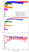 |
Fig. 9. Shape and size of the cavity around the binary (with q = 0.5) and the tranferred specific angular momentum js as a function of time for models with different viscosity and an aspect ratio h = 0.1. Top two panels show sliding time averages over 10 Tbin, the bottom panel shows 200 Tbin for the two lowest α models, over 100 Tbin for α = 0.01, and over 50 Tbin for α = 0.03 and 0.1. The grey lines indicate the averaging interval for the final quoted equilibrium values. Simulations were performed with the RH2D code. |
The corresponding evolution of the normalised angular momentum accretion onto the binary is displayed in the bottom panel of Fig. 9. To obtain the final js value, we averaged over the length marked in grey and obtained the quoted values. The averaging time increases for lower viscosities because the data are noisier. During the initial cavity filling phase, js is negative because the gravitational torques dominate the inflow of angular momentum  , as seen for example in Muñoz et al. (2020) and Tiede et al. (2020). Again, the approach to equilibrium proceeds on the same (long) viscous timescales, and the final values show a monotonic drop with viscosity.
In Fig. 10 we display the obtained js as a function of viscosity for the two different codes we used (RH2D and PLUTO). Both series show a very similar behaviour, an increase in angular momentum transfer to the binary with increasing viscosity. Results extracted from Muñoz et al. (2020) are overplotted, which are slightly lower than ours. The deviations in js could be caused by numerical differences such as time steps or different grid structures as Muñoz et al. (2020) used mesh-refined grids, but might also be the result of the uncertainty in the measurement of js. However, all models agree in the fundamental finding that thick discs with h = 0.1 lead to expanding orbits even for viscosities as low as α = 10−3.
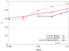 |
Fig. 10. Specific angular momentum js transferred to the binary (with q = 0.5) as a function of the viscosity with an aspect ratio of h = 0.1. The red data points and lines refer to the models in this work using two different codes, and the blue points and line refer to the results of Muñoz et al. (2020). |
5.2. Models with constant viscosity
To allow an individual and independent variation of viscosity and disc scale height, we ran a series of models using a constant kinematic viscosity ν and varied disc thickness and mass ratio. We studied two different values of ν. First, we took the same value as Tiede et al. (2020)
![Mathematical equation: $ \nu = \sqrt{2} \times 10^{-3}\,[a^2\,\Omega_{\mathrm{bin}}] $](/articles/aa/full_html/2022/04/aa41399-21/aa41399-21-eq32.gif) , which allows a direct comparison to their work, and then a value ten times lower. The chosen ν refers to α values of 0.1 and 0.01 at a distance of r = a for H/r = 0.1. In Fig. 11js is displayed as a function of the disc Mach number (=r/H) for a binary with our standard mass ratio q = 0.5 for the two different viscosities. For both viscosity values, we find that js decreases with Mach number and becomes negative for Mach numbers between 30 and 33. This implies that in thin discs, the binary orbit expands, where the turning point lies around a Mach number of 23–25, given by the point at which the curves cross the dash-dotted grey line denoted js,crit = 0.43, calculated for a mass accretion ratio of f = 1.6. See Appendix B.1 for a discussion of the mass accretion ratio.
, which allows a direct comparison to their work, and then a value ten times lower. The chosen ν refers to α values of 0.1 and 0.01 at a distance of r = a for H/r = 0.1. In Fig. 11js is displayed as a function of the disc Mach number (=r/H) for a binary with our standard mass ratio q = 0.5 for the two different viscosities. For both viscosity values, we find that js decreases with Mach number and becomes negative for Mach numbers between 30 and 33. This implies that in thin discs, the binary orbit expands, where the turning point lies around a Mach number of 23–25, given by the point at which the curves cross the dash-dotted grey line denoted js,crit = 0.43, calculated for a mass accretion ratio of f = 1.6. See Appendix B.1 for a discussion of the mass accretion ratio.
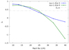 |
Fig. 11. Specific angular momentum js transferred to the binary as a function of the disc Mach number for models with two different values of the kinematic viscosity for a mass ratio q = 0.5. The dash-dotted line refers to a critical js,crit = 0.43. |
In addition to their study, we the varied the mass ratio (ranging from q = 0.33 to q = 1.0), and display our results in Fig. 12. We find the trend that lower mass ratios q lead to an increase in js, while the general behaviour of decreasing js with increasing Mach number is not impacted significantly by changing q. Determining the transition point between expansion and shrinkage for the values of q ≠ 1 requires knowledge of the mass accretion factor f. For a rough estimate, we added the dash-dotted line, which refers to js,crit = 3/8 for q = 1. The true values for the other q will be only slightly higher, as argued in Appendix B.1. For equal-mass binaries, we find an orbit expansion for thicker discs with Mach numbers smaller than ∼20. To compare to earlier results, we overplot the results of Tiede et al. (2020) obtained for q = 1 (dashed black line). While the general trend is similar, the absolute values differ, possibly due to the different numerical methods applied. Our simulations are 2D on a cylindrical grid that does not contain the binary, while theirs are 2D Cartesian.
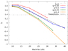 |
Fig. 12. Specific angular momentum js transferred to the binary as a function of the disc Mach number. We present models with a constant kinematic viscosity, |
5.3. Parameter space of H/r and α
Here, we extended our parameter study to standard α-disc models models using five different values α = [0.1, 0.03, 0.01, 0.003, 0.001] and three different aspect ratios H/r = [0.1, 0.05, 0.04] for mass ratios of q = 0.5 and q = 1. As explained in Sect. 5.1, we ran all the models long enough to reach a quasi-stationary equilibrium state with constant acav, ecav, and js.
In Fig. 13 we show the results for q = 1 obtained with the two different codes PLUTO and RH2D. As already shown in Sect. 5.2, for a thick disc with h = 0.1, expanding binary orbits are possible for all values of the viscosity (at least down to α = 0.001). This is due to the fact that in thick discs, the high pressure leads to a continuous refill of the inner cavity at a high rate, carrying a significant amount of angular momentum with it. For thinner discs, the pressure effect is reduced and the viscosity, which scales with h2, and the resulting js values become lower, so that the possibility of expanding orbits is reduced. The lowest aspect ratio, h = 0.04, results only in shrinking binary orbits, similar to what we discussed in Sect. 5.2 for the case of constant viscosities. For h = 0.05, an expanding orbit is only possible for a small window of viscosities between α = 0.01 and 0.1. We find a maximum in js for α ≈ 0.03 and a steep decrease of js towards lower viscosities.
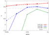 |
Fig. 13. Specific angular momentum js transferred to the binary as a function of the disc viscosity for a mass ratio q = 1.0 and different aspect ratios. For q = 1, the critical rate is given by js, crit = 3/8. We display the results for the two different codes RH2D (crosses, solid lines) and PLUTO (asterisks, dashed lines). |
In systems with a mass ratio of q = 0.5, as shown in Fig. 14, the same trends apply. The denoted js,crit corresponds to an accretion ratio f = 1.6, as motivated by our accretion studies presented in Appendix B.1. The overall shape of the curves is very similar to the q = 1 case. For high viscosities α ≥ 0.01, the values for js lie above the q = 1 case, but as js,crit is also increased, the possible parameter range in which orbit expansion is possible remains the same as in the case of equal-mass binaries.
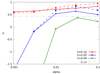 |
Fig. 14. Specific angular momentum js transferred to the binary as a function of the disc viscosity for a mass ratio q = 0.5 and different aspect ratios, using the same notation as in Fig. 13. For the critical rate, we assumed here q = 0.5 and f = 1.6 and obtain js, crit = 0.43. |
For our two model sequences q = 1.0 and 0.5, shown in Figs. 13 and 14, we performed comparison simulations for the thicker discs with h = 0.1 and 0.05 with our two grid codes. In general, the agreement between the two codes is very good. Both show an identical behaviour upon changing the disc viscosity and scale height, even though the absolute values show some differences. Only for the lowest viscosity, α = 10−3, are the differences more pronounced, but these models suffer more from numerical effects such as density floor or diffusion.
In the analysis for very low viscosities, the uncertainties in the measured and averaged js increase, and a much longer time evolution of several ≥10 000 Tbin is needed to reach a stable state of the disc. Additionally, the finite-density floor begins to affect the results due to the very low density in the cavity. Even given these challenges in the simulations, the general picture emerges that low viscosities and low aspect ratios lead to shrinking binary orbits as the cavities become very deep and the advected angular momentum decreases.
5.4. Infinite disc models
The models discussed so far suffer from the problem that no genuine global stationary state is reached. To investigate a different physical setup and determine possible shortcomings of this approach, we ran additional models using an infinite disc setup, in which we covered the full viscosity range for the q = 0.5, H/R = 0.05 model in different numerical resolutions. To model an infinite disc, rout in Eq. (11) was set to very high values, implying that gout → 1. At the same time, we applied damping boundary conditions such that the density at rmax = 40 was always damped towards the initial state (de Val-Borro et al. 2006), while the velocities were kept at their original values. This setup allows a quasi-stationary equilibrium state to be reached and is hence comparable to the infinite disc models of Muñoz et al. (2020). Due to the outflow condition at the inner boundary, at rmin = a, there is a mass flow through the disc and the (time-averaged) mass accretion will be radially constant; see also Kley & Haghighipour (2014). It is crucial to set a very low density floor in the models because the low-viscosity simulations can reach very low densities inside the cavity. Here, we used floor values as low as 10−10 of the initial Σ(r = 1).
The resulting js is shown in Fig. 15, where we display results for the finite torus models from above (red data labelled ‘finite’) and new simulations using the ‘infinite’ disc setup at two different grid resolutions, the standard 684 × 584 (blue dashed) and a higher resolution 968 × 824 case (green dotted). To save computational time, the higher-resolution models were not started from t = 0, but were continued from the standard resolution runs at a time when those reached approximately their equilibrium state. All simulations in Fig. 15 followed the same overall trends, but differ in the actual values of js. Concerning js, we find an increase for the higher-resolution runs for the lower viscosities, but it is not sufficient to lead to an expansion of the binary because the values consistently lie below js,crit. We confirm the finding of Muñoz et al. (2020) that the outer boundary does not significantly change the inner angular momentum transport that is relevant for the binary. Additional tests for H/R = 0.05, α = 0.003 with an even higher resolution showed no further changes in js, and the shrinking of the binary appears to be real for very low viscosities.
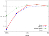 |
Fig. 15. Comparison of the normalised angular momentum accretion, js, for a model with q = 0.5 and H/R = 0.05 for torus-like (finite) and infinite disc models using the standard (684 × 584) vs. higher (968 × 824) grid resolutions. |
For our locally isothermal infinite disc models in quasi-equilibrium for which the density at the outer boundary was fixed, the mass accretion rate should scale linearly with the viscosity according to the classic relation Ṁ = 3πνΣ. In the top panel of Fig. 16, we plot the mass accretion rate onto the binary (measured at rmin) as a function of α for models with q = 0.5 and h = 0.05 at two numerical resolutions, using the line style of Fig. 15. Except for the lowest α values, the expected linear relation (grey line) is well satisfied, but the agreement with the linear relation improves with higher grid resolution. The bottom panel of Fig. 16 shows the absolute value of the two contributions to  , the gravitational part (
 , green and blue lines), and the advective part (
 , in grey). The gravitational term removes angular momentum from the binary, while the advection term adds angular momentum to it. The two advective terms
  and Ṁadv follow the same slope, such that the advective
  is almost constant at a value of 1.25 ± 0.04 upon varying the viscosity. It has a lowest value of ∼1.21 for α = 0.003 and increases to ∼1.27 for α = 0.1, and is ∼1.23 for the smallest α = 0.001. At the same time, the gravitational contribution
  flattens towards lower viscosities and equals the advective part for α ∼ 0.002, making the total js negative, as shown in Fig. 15.
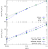 |
Fig. 16. Mass accretion rate onto the binary as a function of viscosity for infinite disc models with q = 0.5 and h = 0.05 (top). The grey line indicates a linear slope. Corresponding absolute value of gravitational (bottom, blue and green lines) and advective (grey lines) angular momentum transfer, |


In order to understand the observed behaviour better, we show in Fig. 17 the 2D surface density distribution for the infinite disc models for the different viscosities. The computed cavity edges are marked by the dashed white ellipses, which were computed with the method described in Thun et al. (2017). Clearly seen are the eccentric inner cavities, which are more pronounced in these thinner discs (h = 5%) compared to the standard model (with h = 10%) even at a logarithmic scale. The cavity’s size and eccentricity are both smallest for the highest viscosity case (α = 10−1) and increase upon lowering α. Maximum values for acav and ecav are reached for intermediate α, and they drop again for even lower viscosities. The logarithmic colour scale helps visualise the streamers and infalling gas inside the cavity. The strength of streamers weakens with reduced viscosity, coinciding with the generally declining trend in the advective angular momentum contribution shown in Fig. 16. As expected, the cavity becomes wider and deeper upon lowering the viscosity. When the viscosity becomes very low, however, this trend is slowed and even reverses. At the same time, with reduced accretion, the mass in the streamers declines and the torque from inside the cavity reduces proportionally. However, the always eccentric disc causes the gravitational contribution in Fig. 16 to change its slope around α = 0.01, aided by the slight contraction of the disc. This results in shrinking binary orbits for the lowest viscosities.
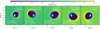 |
Fig. 17. Snapshots of the surface density for infinite disc models with q = 0.5 and H/R = 0.05 for different viscosities, ranging from α = 0.1 (left) to α = 0.001 (right). We show the inner region of the disc for the higher-resolution models in their final state at the times indicated. The dashed white lines indicate the ellipses fitted to the cavity with the parameters quoted. The blue dots mark the position of the stars. |
6. Discussion and conclusion
We presented 2D hydrodynamical simulations of discs around a circular binary where disc and binary are coplanar. We monitored the mass and angular momentum balance of the disc in order to calculate the orbital evolution of the binary. Our prime interest was to evaluate shrinkage or expansion of the binary by determining the sign of the semi-major axis evolution for different mass ratios of the binary and various disc parameters. Based on the assumption that the binary orbit remains circular under this accretion process, we showed that its change in semi-major axis due to the mass and angular momentum transfer between circumbinary disc and binary is directly proportional to the mass accretion rate times a function that depends on the stellar mass ratio q, the specific angular momentum transfer js, and the relative mass accretion onto the binary f; see Eq. (8).
In agreement with the studies of Miranda et al. (2017), our simulations show that the specific angular momentum transfer rate js serves as an eigenvalue of the problem that can be calculated using a cylindrical grid with an inner hole with a radius of rin ∼ abin, that is, the grid does not contain the central binary system. Additionally, we confirm results of Muñoz et al. (2020) that in order to obtain a quasi-equilibrium for js it is sufficient to model a torus-like configuration with limited radial extent because it is sufficient to bring the inner disc regions into equilibrium and not the whole disc. This finding is supported by additional simulations using an infinite disc setup that allows for a global stationary state with resulted in js values very similar to those from the torus models.
While for q = 1 the critical value is given by js,crit = 3/8, for all q ≠ 1 knowledge of f is required to find the exact threshold 0 < js,crit < 1. In the work of Muñoz et al. (2020), the mass accretion ratio of systems with q = 0.5 averages f ≈ 1.5, which is consistent with the trend in Dittmann & Ryan (2021). In order to compare, we performed supplemental simulations covering the whole domain in the appendix using Cartesian grids and the SPH method. We found that for a mass ratio of q = 0.5, the mass accretion ratio lies somewhere between 1.3 and 1.8, that is, the secondary star accretes more mass from the disc than the primary. As these studies are very time consuming and depend on numerical treatments such as potential smoothing, sink radii, and others, we leave more detailed analyses to future studies for the full range of parameters.
Using an average value f = 1.6, we showed for two mass ratios (q = 1 and 0.5) that binaries expand for sufficiently high viscosity, α ≥ 0.01 and disc aspect ratios, h ≥ 0.05. For thinner and less viscous discs, the binaries tend to shrink. Thick discs with h = 0.1 result in expansion for all viscosities, while discs with h = 0.05 show expansion for α larger than ∼0.005. Independent of the mass ratio, we find that thin and low-viscosity discs cause the binary orbit to shrink. Only thick and highly viscous discs can lead to expanding binary orbits.
For our simulations, we assumed a coplanar configuration in which the disc and binary lie in the same plane. This is motivated by the observed coplanar distribution of detected circumbinary planets and the fact that the inner disc will align towards the binary plane over time, see for instance Pierens & Nelson (2018). Additionally, we restricted ourselves to a 2D treatment and neglected the vertical disc structure. Only this simplification allowed us to perform the simulations over viscous timescales. The aligned 3D SPH model in Hirsh et al. (2020) produced comparable cavity structures and sizes as 2D models, and therefore we expect that the restriction to a 2D setup can produce realistic results.
In our models we kept the binary stars on a fixed orbit. Muñoz et al. (2019) evaluated the binary migration rate ȧ/a in a dynamic model and reported that it was on the order of twice the mass accretion rate for the α = h = 0.1 case. For even lower viscosities, the migration accordingly is considerably slower. We tested ȧ/a in the disc structure caused by the gravitational term  and found no deviations with or without “live” binaries in the simulations for various viscosities. We did not include the momentum transfer onto the binary stars in this study because it is not computationally feasible to create models with a far lower viscosity that include the motion of the binaries directly because of the very long convergence time that is needed.
In Eq. (8) we omitted the eccentricity term as we only studied circular binaries. If the change in eccentricity were considered as well, it would lead to a second variable to solve for, and the resulting equation would not be solvable with just angular momentum conservation. The additional property to look for is the momentum change of the binary induced by the mass accretion, which can only be computed if the stars are contained within the computational domain. This is not feasible for current models.
As circular binaries represent a configuration with maximum angular momentum for a given semi-major axis, we might expect as a consequence that positive angular momentum transfer will always keep the orbit circular. Models with live binaries indeed show that the induced eccentricity remains very low for initially circular orbits (see e.g. Muñoz et al. 2019; Heath & Nixon 2020). Through the simple prescription of a locally isothermal environment, the model is simple, but scalable. This allows general parameter studies for diverse astronomical discs. When a specific system is examined, a radiative model that includes viscous heating and possibly irradiation can be more physical. In Kley et al. (2019) we tested viscously heated and radiatively cooled circumbinary discs using the parameters of the Kepler-38 and Kepler-16 systems. We found that the locally isothermal assumption with a flat aspect ratio between 4% and 5% for the inner disc provides a good approximation to the more realistic case.
In the models with low viscosities, the accretion of mass and angular momentum becomes very small due to the large cavity size and long viscous evolution timescales. This also implies that the occurring temporal variations in the accretion rate result in stronger fluctuations of the measured js. Therefore, to obtain the mean js, we have to calculate a rolling average over a longer time interval, up to 100 Tbin, or 1000 outputs if obtained from individual snapshot. Still, js for α = 10−3 varies over ±0.2. Nevertheless, our result that for low-viscosity thin discs the binary orbits shrink seems to be robust as the decline of js is much larger than these fluctuations. Since for low values of viscosity and H/r the numerical effects may affect the results, we ran additional simulations using higher grid resolutions and in addition, an infinite disc setup. The results, presented in Sect. 5.4, show that js increases for higher resolutions, but not enough to change our conclusion.
We considered the binary as a point-like gravitational source. However, the planet-hosting Kepler binary systems are close binaries that in addition to the disc impact are influenced by tidal interactions between the stars. In a theoretical study of Kepler 47b (Graham et al. 2021), the binary stars have roughly a semi-major axis change of 0.5% over 109 years. This would be a much slower change than the effect we see from the disc. We can therefore safely assume that the disc is dominant in changing the semi-major axis even for these types of close binaries.
Overall, the regime of binary expansion extends to a much wider parameter space than previously anticipated. This will have consequences with respect to the orbital evolution of binary black holes prior to merger or the evolution of stellar binaries in their formation phase. These results for very low disc thicknesses and viscosities are somewhat preliminary as our numerical resolution may not have been high enough to cover these cases properly. Additional simulations using higher numerical resolution suggest that js increases, which could imply that the range of binary expansion will be somewhat larger. This does not change our conclusion of shrinking binaries for low α and small H/r.
Future simulations need to address more realistic physical conditions that include radiative effects. The geometry needs to be extended to full 3D to verify the thin-disc approach because recent simulations of massive embedded planet in discs point towards a discrepancy between 2D and 3D simulations with respect to the eccentricity of the outer disc (Li et al. 2021).
Acknowledgments
During the course of the revision of this paper, our colleague Willy Kley passed away unexpectedly. We want to express our sincere gratitude to him, who was not only our mentor, but also a dear and supportive friend. Thank you, Willy! Anna Penzlin and Hugo Audiffren were both funded by grant 285676328 from the German Research Foundation (DFG). The authors acknowledge support by the High Performance and Cloud Computing Group at the Zentrum für Datenverarbeitung of the University of Tübingen, the state of Baden-Württemberg through bwHPC and the German Research Foundation (DFG) through grant no INST 37/935-1 FUGG. Some of the plots in this paper were prepared using the Python library matplotlib (Hunter 2007).
References
- Artymowicz, P., & Lubow, S. H. 1994, ApJ, 421, 651 [Google Scholar]
- Artymowicz, P., Clarke, C. J., Lubow, S. H., & Pringle, J. E. 1991, ApJ, 370, L35 [NASA ADS] [CrossRef] [Google Scholar]
- Begelman, M. C., Blandford, R. D., & Rees, M. J. 1980, Nature, 287, 307 [Google Scholar]
- de Val-Borro, M., Edgar, R. G., Artymowicz, P., et al. 2006, MNRAS, 370, 529 [Google Scholar]
- Dittmann, A. J., & Ryan, G. 2021, ApJ, 921, 71 [NASA ADS] [CrossRef] [Google Scholar]
- Duffell, P. C., D’Orazio, D., Derdzinski, A., et al. 2020, ApJ, 901, 25 [NASA ADS] [CrossRef] [Google Scholar]
- Flebbe, O., Muenzel, S., Herold, H., Riffert, H., & Ruder, H. 1994, ApJ, 431, 754 [Google Scholar]
- Graham, D. E., Fleming, D. P., & Barnes, R. 2021, A&A, 650, A178 [NASA ADS] [CrossRef] [EDP Sciences] [Google Scholar]
- Heath, R. M., & Nixon, C. J. 2020, A&A, 641, A64 [NASA ADS] [CrossRef] [EDP Sciences] [Google Scholar]
- Hirsh, K., Price, D. J., Gonzalez, J.-F., Ubeira-Gabellini, M. G., & Ragusa, E. 2020, MNRAS, 498, 2936 [NASA ADS] [CrossRef] [Google Scholar]
- Hunter, J. D. 2007, Comput. Sci. Eng., 9, 90 [NASA ADS] [CrossRef] [Google Scholar]
- Kley, W. 1989, A&A, 208, 98 [NASA ADS] [Google Scholar]
- Kley, W. 1999, MNRAS, 303, 696 [NASA ADS] [CrossRef] [Google Scholar]
- Kley, W., & Haghighipour, N. 2014, A&A, 564, A72 [NASA ADS] [CrossRef] [EDP Sciences] [Google Scholar]
- Kley, W., Thun, D., & Penzlin, A. B. T. 2019, A&A, 627, A91 [NASA ADS] [CrossRef] [EDP Sciences] [Google Scholar]
- Li, Y.-P., Chen, Y.-X., Lin, D. N. C., & Zhang, X. 2021, ApJ, 906, 52 [NASA ADS] [CrossRef] [Google Scholar]
- Mignone, A., Bodo, G., Massaglia, S., et al. 2007, ApJS, 170, 228 [Google Scholar]
- Milosavljević, M., & Merritt, D. 2003, in The Astrophysics of Gravitational Wave Sources, ed. J. M. Centrella, AIP Conf. Ser., 686, 201 [CrossRef] [Google Scholar]
- Miranda, R., & Lai, D. 2015, MNRAS, 452, 2396 [Google Scholar]
- Miranda, R., Muñoz, D. J., & Lai, D. 2017, MNRAS, 466, 1170 [NASA ADS] [CrossRef] [Google Scholar]
- Monaghan, J. 1989, J. Comput. Phys., 82, 1 [NASA ADS] [CrossRef] [Google Scholar]
- Moody, M. S. L., Shi, J.-M., & Stone, J. M. 2019, ApJ, 875, 66 [NASA ADS] [CrossRef] [Google Scholar]
- Muñoz, D. J., Miranda, R., & Lai, D. 2019, ApJ, 871, 84 [CrossRef] [Google Scholar]
- Muñoz, D. J., Lai, D., Kratter, K., & Miranda, R. 2020, ApJ, 889, 114 [Google Scholar]
- Penzlin, A. B. T., Kley, W., & Nelson, R. P. 2021, A&A, 645, A68 [NASA ADS] [CrossRef] [EDP Sciences] [Google Scholar]
- Pierens, A., & Nelson, R. P. 2018, MNRAS, 477, 2547 [NASA ADS] [CrossRef] [Google Scholar]
- Schäfer, C., Speith, R., Hipp, M., & Kley, W. 2004, A&A, 418, 325 [NASA ADS] [CrossRef] [EDP Sciences] [Google Scholar]
- Schäfer, C., Riecker, S., Maindl, T. I., et al. 2016, A&A, 590, A19 [NASA ADS] [CrossRef] [EDP Sciences] [Google Scholar]
- Schäfer, C. M., Wandel, O. J., Burger, C., et al. 2020, Astron. Comput., 33, 100410 [CrossRef] [Google Scholar]
- Thun, D., & Kley, W. 2018, A&A, 616, A47 [NASA ADS] [CrossRef] [EDP Sciences] [Google Scholar]
- Thun, D., Kley, W., & Picogna, G. 2017, A&A, 604, A102 [NASA ADS] [CrossRef] [EDP Sciences] [Google Scholar]
- Tiede, C., Zrake, J., MacFadyen, A., & Haiman, Z. 2020, ApJ, 900, 43 [NASA ADS] [CrossRef] [Google Scholar]
- Zrake, J., Tiede, C., MacFadyen, A., & Haiman, Z. 2021, ApJ, 909, L13 [NASA ADS] [CrossRef] [Google Scholar]
Appendix A: Code comparison
In order to validate complex hydrodynamical simulations, it is very helpful if not mandatory to perform simulations using completely different numerical approaches on the same physical problem. Even though in this paper we have compared the two grid codes for a wider parameter range, it is usually prohibited to do this for all different choices of parameter. Hence, we chose our standard model and performed simulations for three different codes: The finite-volume codes PLUTO and RH2D, and an SPH code. The first code we used is a full GPU version of the hydrodynamical part of the PLUTO code (Mignone et al. 2007) as described in Thun et al. (2017). It is a Riemann-solver-based finite-volume code, where we used the van Leer limiter for the reconstruction and a second-order time-stepping. As an alternative grid code, we used RH2D, which is a classic second-order upwind code working on a staggered grid (Kley 1989, 1999), again using the van Leer limiter for the slopes.
For the SPH simulations, we used the GPU code miluphcuda (Schäfer et al. 2016, 2020). In the standard model, we chose the same inner and outer boundary radius of the computational domain as the grid simulations, 1a to 40a. Particles that cross the inner or outer boundary during the simulation were taken out of the computation. All particles had the same mass and were distributed in the beginning to represent the initial density profile. The initial smoothing lengths of the particles were chosen to ensure an overall constant number of interactions and to match the density profile. We applied variable smoothing and integrated the smoothing length using the standard approach (in 2D)
 (A.1)
(A.1)
where hSPH is the smoothing length and v is the velocity. The code solves the Navier-Stokes equations following the scheme by Flebbe et al. (1994), where the kinematic viscosity is given by the α model (see above). Additionally, an artificial bulk viscosity was applied following Schäfer et al. (2004), and the XSPH algorithm for additional smoothing of the particle velocities was used (Monaghan 1989). The standard setup initially included 500 000 particles.
All three simulations started from the same initial setup and were run for at least 600 Tbin. In Fig. A.1 we show the time evolution for mass accretion and angular momentum change of the disc, and the specific angular momentum transfer js. The results for the RH2D code are identical to those displayed in Fig. 5 above. The two grid-based codes show an excellent agreement for all three variables throughout the whole evolution. The SPH code has a slightly lower mass and angular momentum transfer, resulting in a lower js, but it lies still well above js,crit. This difference might be caused by the different treatment of the viscosity in SPH. In the very low density region in the inner parts of the disc near the central binary, there are fewer particles, which might lead to an inaccurate estimate of the viscosity. In Fig. A.2 we compare the azimuthally averaged radial density profile after 500 Tbin. The results of all codes are almost perfectly aligned, except for highly dynamic spiral features in the density profile in the central regions. At the inner boundary, the SPH code has a slightly higher density, but the position of the density maximum, the onset of the spiral features, and the density of in the outer disc match well in all models. In particular, it is worth noting that the viscous outward spreading of the initial torus is identical for all three codes, indicating identical viscosity. We conclude that (at least for the standard model) the physical behaviour and our conclusion about the binary evolution is robust.
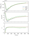 |
Fig. A.1. Mass accretion, angular momentum change of the disc, and resulting js over time for our two grid codes PLUTO (solid blue), RH2D (dashed orange), and the SPH code miluphcuda (dash-dotted green). |
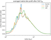 |
Fig. A.2. Azimuthally averaged surface density profile at 500 binary orbits of our two grid codes PLUTO (blue) and RH2D (orange), and the SPH code miluphcuda (green). |
Appendix B: Estimating the accretion ratio
Here, we briefly present our initial studies to estimate the accretion factor f. For this purpose, we used two different approaches. First, the grid-code RH2D, now in a Cartesian setup, and secondly, the particle-based SPH-code miluphcuda.
B.1. Cartesian grid simulation
To calculate the orbital evolution of the binary, an estimate of the accretion factor, f, that is, the mass accretion ratio onto the two stars, is required. As this is not possible for a cylindrical grid, which has an inner hole at rmin, we additionally ran Cartesian simulations using the two grid codes. We covered a domain of [ − 20 : 20, −20 : 20] for the standard model with a Cartesian grid using different numbers of grid cells, ranging from 1200 × 1200 up to 4800 × 4800. In deviation from the standard model, we used a constant (dimensionless) viscosity of ν = 1.41 × 10⁻³ to avoid problems in defining suitable disc thicknesses in the vicinity of the two stars. The initial density distribution was identical to the standard model, using rin = 2.5 and rout = 6. For the stellar potentials, we used a Plummer-type smoothing with rsm1 = 0.15 M1 and rsm2 = 0.15 M2 for the two stars. For the sink radii, we use 2/3 rsm for the two stars. Inside the sink radii of the two stars, mass was taken out at a half-emptying time of τ1/2 ∼ 7 Tbin.
The 2D density distribution of this Cartesian simulation is displayed in Fig. B.1 for the standard model after a simulated time of 500 Tbin. Despite the accretion of mass, the circumstellar discs are still visible around both stars, implying that the relatively short τ1/2 is not effective enough to remove the circumstellar discs entirely. From these simulations, we can obtained the mass accretion rates on the two stars and the important accretion ratio, f. We did not monitor the angular momentum transfer to the stars in these simulations and leave this to future studies.
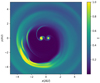 |
Fig. B.1. Density structure in the central region for the RH2D model with 3400 × 3400 cells with the parameters of the standard model after 500 binary periods. |
The measured accretion ratio for q = 0.5 onto the stars is displayed in Fig. B.2 for different grid resolutions. The models settle to an equilibrium at about 250 to 300 Tbin, after which the accretion ratios remain approximately constant. Increasing the grid resolution increases the accretion factor, and the results converge for the standard model against a value flim ≈ 1.37. As a test for the accretion procedure, we performed the same simulation for a model with two equal-mass stars (q = 1, α = 0.1, and h = 0.1) and found a mass accretion ratio f = 1, meaning equal accretion onto both stars, as expected.
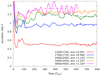 |
Fig. B.2. Stellar mass accretion ratio, f = Ṁ2/Ṁ1, onto the two stars for Cartesian simulations with different grid resolutions. We show the time evolution with the corresponding averages, taken over the time interval indicated by the dashed lines. |
B.2. SPH-Miluphcuda
For the SPH simulations conducted in this project, we defined individual accretion radii around the stars that scaled with the corresponding mass. Whenever a particle crossed the accretion radius of a star, we monitored its mass, velocity, and accretion time and removed it from the simulation. However, we chose the accretion radii small enough to prevent overlapping, that is, racc1 = 0.1 M1 and racc2 = 0.1 M2.
The 2D density distribution of the model after a time t = 500 Tbin is shown in Fig. B.3. The overall structure is very comparable to the results of the cylindrical and Cartesian grid models with similar cavity size. The density distribution was calculated by interpolating the particles to a cylindrical grid such that the same analysis tools could be used as for the grid codes. The SPH accretion ratio is plotted in Fig. B.4, and the mean value fSPH, mean ≈ 1.86 is computed over the last 200 orbits.
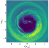 |
Fig. B.3. Density structure in the central region for the SPH model with the parameters of the standard model using 5 × 10⁵ particles after 500 binary periods. For the colour scaling, see Fig. B.1. |
In our parameter study, we used an average f = 1.6 for the relative mass accretion rates to calculate the critical js,crit, assuming that a similar value will be taken for other values of α and h. This value agrees well with the recent study by Dittmann & Ryan (2021), who performed a more detailed analysis of mass and angular momentum accretion using different numerical recipes, and with Muñoz et al. (2020), who used the moving mesh code AREPO and found a slightly higher accretion ratio of ∼1.7 after about 400 orbits for similar disc and binary parameters (see their Fig. 9).
All Tables
All Figures
|
Fig. 1. Critical angular momentum transfer to the binary as a function of the binary mass ratio for different values of the accretion factor; see Eq. (9). If the binary receives angular momentum at a rate higher than js, crit, then its orbit expands. We display five different values for the factor f that enclose all cases between the two limiting cases of f = 0 (accretion only on the primary) and f → ∞ (accretion only on the secondary). |
| In the text | |
|
Fig. 2. Azimuthally averaged surface density for the standard model (q = 0.5, h = 0.1, α = 0.1) at five different times, quoted in binary orbits. |
| In the text | |
|
Fig. 3. 2D surface density distribution at 500 Tbin for the standard setup. The black cross marks the binary barycenter, and the region within r = 1 abin is not part of the computational domain. |
| In the text | |
|
Fig. 4. Approximated cavity size and eccentricity for the standard model. The curves denoted ‘averaged’ denote the sliding averages over ten orbits for three different codes. The grey dots show the instantaneously estimated values. |
| In the text | |
|
Fig. 5. Loss and gain channels of mass and angular momentum, Ṁ and |
| In the text | |
|
Fig. 6. Specific angular momentum transfer, js, onto the binary for the standard model. The curve represents a sliding average over ten orbits, and the grey line shows the average over the last 1000 orbits. |
| In the text | |
|
Fig. 7. Azimuthally averaged density for five different inner grid radii rmin after 500 binary orbits for simulations using the PLUTO code. |
| In the text | |
|
Fig. 8. Evolution of mass and angular momentum gain and loss rates of the disc and of js for different inner disc radii, computed using the PLUTO code. The dashed lines in the bottom panel indicate the obtained average values between 200 − 700 Tbin. |
| In the text | |
|
Fig. 9. Shape and size of the cavity around the binary (with q = 0.5) and the tranferred specific angular momentum js as a function of time for models with different viscosity and an aspect ratio h = 0.1. Top two panels show sliding time averages over 10 Tbin, the bottom panel shows 200 Tbin for the two lowest α models, over 100 Tbin for α = 0.01, and over 50 Tbin for α = 0.03 and 0.1. The grey lines indicate the averaging interval for the final quoted equilibrium values. Simulations were performed with the RH2D code. |
| In the text | |
|
Fig. 10. Specific angular momentum js transferred to the binary (with q = 0.5) as a function of the viscosity with an aspect ratio of h = 0.1. The red data points and lines refer to the models in this work using two different codes, and the blue points and line refer to the results of Muñoz et al. (2020). |
| In the text | |
|
Fig. 11. Specific angular momentum js transferred to the binary as a function of the disc Mach number for models with two different values of the kinematic viscosity for a mass ratio q = 0.5. The dash-dotted line refers to a critical js,crit = 0.43. |
| In the text | |
|
Fig. 12. Specific angular momentum js transferred to the binary as a function of the disc Mach number. We present models with a constant kinematic viscosity, |
| In the text | |
|
Fig. 13. Specific angular momentum js transferred to the binary as a function of the disc viscosity for a mass ratio q = 1.0 and different aspect ratios. For q = 1, the critical rate is given by js, crit = 3/8. We display the results for the two different codes RH2D (crosses, solid lines) and PLUTO (asterisks, dashed lines). |
| In the text | |
|
Fig. 14. Specific angular momentum js transferred to the binary as a function of the disc viscosity for a mass ratio q = 0.5 and different aspect ratios, using the same notation as in Fig. 13. For the critical rate, we assumed here q = 0.5 and f = 1.6 and obtain js, crit = 0.43. |
| In the text | |
|
Fig. 15. Comparison of the normalised angular momentum accretion, js, for a model with q = 0.5 and H/R = 0.05 for torus-like (finite) and infinite disc models using the standard (684 × 584) vs. higher (968 × 824) grid resolutions. |
| In the text | |
|
Fig. 16. Mass accretion rate onto the binary as a function of viscosity for infinite disc models with q = 0.5 and h = 0.05 (top). The grey line indicates a linear slope. Corresponding absolute value of gravitational (bottom, blue and green lines) and advective (grey lines) angular momentum transfer, |
| In the text | |
|
Fig. 17. Snapshots of the surface density for infinite disc models with q = 0.5 and H/R = 0.05 for different viscosities, ranging from α = 0.1 (left) to α = 0.001 (right). We show the inner region of the disc for the higher-resolution models in their final state at the times indicated. The dashed white lines indicate the ellipses fitted to the cavity with the parameters quoted. The blue dots mark the position of the stars. |
| In the text | |
|
Fig. A.1. Mass accretion, angular momentum change of the disc, and resulting js over time for our two grid codes PLUTO (solid blue), RH2D (dashed orange), and the SPH code miluphcuda (dash-dotted green). |
| In the text | |
|
Fig. A.2. Azimuthally averaged surface density profile at 500 binary orbits of our two grid codes PLUTO (blue) and RH2D (orange), and the SPH code miluphcuda (green). |
| In the text | |
|
Fig. B.1. Density structure in the central region for the RH2D model with 3400 × 3400 cells with the parameters of the standard model after 500 binary periods. |
| In the text | |
|
Fig. B.2. Stellar mass accretion ratio, f = Ṁ2/Ṁ1, onto the two stars for Cartesian simulations with different grid resolutions. We show the time evolution with the corresponding averages, taken over the time interval indicated by the dashed lines. |
| In the text | |
|
Fig. B.3. Density structure in the central region for the SPH model with the parameters of the standard model using 5 × 10⁵ particles after 500 binary periods. For the colour scaling, see Fig. B.1. |
| In the text | |
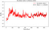 |
Fig. B.4. Evolution of the accretion ratio for the SPH model shown in Fig. B.3. |
| In the text | |
Current usage metrics show cumulative count of Article Views (full-text article views including HTML views, PDF and ePub downloads, according to the available data) and Abstracts Views on Vision4Press platform.
Data correspond to usage on the plateform after 2015. The current usage metrics is available 48-96 hours after online publication and is updated daily on week days.
Initial download of the metrics may take a while.