| Issue |
A&A
Volume 660, April 2022
|
|
|---|---|---|
| Article Number | A82 | |
| Number of page(s) | 16 | |
| Section | Extragalactic astronomy | |
| DOI | https://doi.org/10.1051/0004-6361/202141260 | |
| Published online | 14 April 2022 | |
APEX and NOEMA observations of H2S in nearby luminous galaxies and the ULIRG Mrk 231
A possible relation between dense gas properties and molecular outflows
1
Department of Space, Earth and Environment, Chalmers University of Technology, Onsala Space Observatory, 439 92 Onsala, Sweden
e-mail: This email address is being protected from spambots. You need JavaScript enabled to view it.
2
Institute of Astronomy, Graduate School of Science, The University of Tokyo, 2-21-1 Osawa, Mitaka, Tokyo 181-0015, Japan
3
National Astronomical Observatory of Japan, 2-21-1 Osawa, Mitaka, Tokyo 181-8588, Japan
4
Leiden Observatory, Leiden University, PO Box 9513, 2300 RA Leiden, The Netherlands
5
Department of Physics and Astronomy, UCL, Gower Street, London WC1E 6BT, UK
Received:
6
May
2021
Accepted:
10
December
2021
Abstract
Context. In order to understand the evolution and feedback of active galactic nuclei (AGN) and star formation, it is important to use molecular lines as probes of physical conditions and chemistry.
Aims. We use H2S to investigate the impact of starburst and AGN activity on the chemistry of the molecular interstellar medium in luminous infrared galaxies. Specifically, our aim is to search for evidence of shock enhancement of H2S related to galactic-scale mechanical feedback processes such as outflows.
Methods. Using the APEX single-dish telescope, we have observed the 110–101 transition of ortho-H2S at 168 GHz towards the centres of 12 nearby luminous infrared galaxies. We have also observed the same line towards the ultra-luminous infrared galaxy Mrk 231 with the NOEMA interferometer.
Results. We detected H2S towards NGC 253, NGC 1068, NGC 3256, NGC 4418, NGC 4826, NGC 4945, Circinus, M 83, and Mrk 231. Upper limits were obtained for NGC 1097, NGC 1377, and IC 860. We also detected line emission from HCN 2–1 in all galaxies in the APEX survey as well as HCO+, HNC, CH3CN, CH3OH, H2CS, HOC+, and SO in several of the sample galaxies. Mrk 231 has a rich 2 mm molecular spectrum and, in addition to H2S, we detect emission from HC3N, CH3OH, HC18O+, C2S, and CH3CCH. Four galaxies show elevated H2S emission relative to HCN: Circinus, NGC 3256, NGC 4826, and NGC 4418. We suggest that the high line ratios are caused by elevated H2S abundances in the dense gas. However, we do not find any clear connection between the H2S/HCN line intensity ratio and the presence (or speed) of molecular outflows in the sample galaxies. Therefore, H2S abundances do not seem to be globally affected by the large-scale outflows. In addition, the H2S/HCN line ratio is not enhanced in the line wings compared to the line core in Mrk 231. This suggests that H2S abundances do not increase in the dense gas in the outflow. However, we do find that the H2S and HCN luminosities (LH2S and LHCN) correlate well with the total molecular gas mass in the outflow, Moutflow(H2), in contrast to LCO and LHCO+. We also find that the line luminosity of H2S correlates with the total infrared luminosity in a similar way as that of H2O.
Conclusions. We do not find any evidence of H2S abundance enhancements in the dense gas due to galactic-scale outflows in our sample galaxies, nor in the high-resolution study of Mrk 231. We discuss possible mechanisms behind the suggested H2S abundance enhancements in NGC 4418, Circinus, NGC 3256, and NGC 4826. These include radiative processes (for example X-rays or cosmic rays) or smaller-scale shocks. Further high-resolution and multi-transition studies are required to determine the cause behind the elevated H2S emission in these galaxies. We suggest that LH2S serves as a tracer of the dense gas content, similar to LHCN, and that the correlation between LH2S and Moutflow(H2) implies a relation between the dense gas reservoir and the properties and evolution of the molecular feedback. This potential link requires further study since it holds important keys to our understanding of how the properties of molecular outflows relate to those of their host galaxies. Finally, the similar infrared-correlation coefficients between H2S and H2O may indicate that they originate in the same regions in the galaxy: warm gas in shocks or irradiated by star formation or an AGN.
Key words: galaxies: evolution / galaxies: nuclei / galaxies: ISM / ISM: molecules / ISM: jets and outflows
Note to the reader: on page 8, 2nd paragraph, the duplicate in the first sentence has been removed on 20 April 2022.
© ESO 2022
1. Introduction
Molecular gas plays an important role in the bursts of star formation and the feeding of super massive black holes (SMBHs), in particular when collisions of gas-rich galaxies funnel massive amounts of material into the nuclei of luminous infrared galaxies (LIRGs) and ultra-luminous infrared galaxies (ULIRGs; Sanders & Mirabel 1996; Iono et al. 2009). Molecular gas probes important physical processes, such as massive outflows powered by the nuclear activity (e.g. Sturm et al. 2011; Feruglio et al. 2011; Chung et al. 2011; Aalto 2012; Aalto et al. 2012, 2015a; Cicone et al. 2014; Sakamoto et al. 2014; Fluetsch et al. 2019; Veilleux et al. 2020). These outflows help to regulate the growth of galaxy nuclei, and the implied outflow momenta suggest that the inner regions of these galaxies may be cleared of material within a few megayears (e.g. Feruglio et al. 2011; Cicone et al. 2014). The morphology of the molecular feedback ranges from wide-angle winds (Veilleux et al. 2013) and gas entrained by radio jets (Morganti et al. 2015; García-Burillo et al. 2015; Dasyra et al. 2016) to collimated molecular outflows (Aalto et al. 2016; Sakamoto et al. 2017; Barcos-Muñoz et al. 2018; Falstad et al. 2019).
The fate of the molecular gas is still not well understood. One question is whether the gas is expelled from the galaxy or returns to fuel another cycle of activity (e.g. Pereira-Santaella et al. 2018; Lutz et al. 2020). It is also not known if the molecular clouds are swept up from a circumnuclear disk or formed in the outflow (e.g. Ferrara & Scannapieco 2016). Another question is whether the clouds expand and evaporate or if they condense and form stars in the outflow (Maiolino et al. 2017). A detailed study of the physical conditions of the molecular gas in outflows is necessary to understand its origin and how it evolves within the outflow, as well as how this is linked to the nature of the driving force.
Important extragalactic probes of cloud properties include molecules such as HCN, HCO+, HNC, CN, and HC3N. These molecules have high dipole moments, which means that they normally require high densities (n > 104 cm−3) for efficient excitation. Hence, they are in general more tightly related to dense star-forming gas compared to low-J transitions of CO, as shown by Gao & Solomon (2004).
The detection of luminous HCN and CN emission in molecular outflows, which are often powered by active galactic nuclei (AGN), is evidence of the presence of large amounts of dense molecular gas (e.g. Aalto 2012; Sakamoto et al. 2014; Matsushita et al. 2015; García-Burillo et al. 2015; Privon et al. 2015; Cicone et al. 2020). However, we should note that faint, but widespread, HCN emission may also emerge from more diffuse gas (e.g. Nishimura et al. 2017).
To understand the origin of the dense gas in outflows, we require tracers that probe specific physical and chemical conditions. One of the most reactive elements is sulphur: its chemistry is very sensitive to the thermal and kinetic properties of the gas. Sulphur-bearing molecules, such as H2S, SO, and SO2, appear to be unusually abundant in clouds with high mass star formation, accompanied by shock waves and/or high temperatures (e.g. Mitchell 1984; Minh et al. 1990). Hence, observations of sulphur-bearing molecules could be used to constrain the properties of the dense gas in outflows.
H2S is often assumed to be the most abundant sulphur-bearing species on ice mantles, as the hydrogenation of sulphur should be very efficient on the dust grains, despite not being detected in interstellar ices (Charnley 1997; Wakelam et al. 2004; Viti et al. 2004). In quiescent star-forming regions, gas-phase abundances of H2S are therefore low because they are depleted on grains.
Strong shocks can sputter H2S off the grains moving into the gas phase. There are many theoretical studies that test this hypothesis (e.g. Woods et al. 2015), giving ample evidence of enhanced gas phase H2S in warm and/or shocked environments. In model calculations, Holdship et al. (2017) have shown that as a C-type shock passes through the cloud, sulphur is first transformed into H2S and its abundance increases greatly in the post-shock gas. H2S chemistry and grain-processing features share several properties with those of water, H2O, but with the added advantage that its ground-state transition occurs at a wavelength of λ = 2 mm and can be observed with ground-based telescopes.
H2S seems to be a promising tracer for probing outflows and dusty nuclear activity in galaxies. Photon-dominated regions (PDRs) may also contribute significantly to the H2S emission (e.g. Goicoechea et al. 2021). Here we present the results of an Atacama Pathfinder Experiment (APEX) single-dish telescope pilot survey of the 168.7 GHz 11, 0–10, 1 transition of H2S towards a sample of galaxies to study the relationship between H2S emission and the outflow activity of the galaxies. We also present 168.7 GHz IRAM Northern Extended Millimeter Array (NOEMA) H2S observations of the nucleus and outflow of the ULIRG merger Mrk 231.
This paper is organised as follows. In Sect. 2 we present the galaxy sample, as well as the APEX and NOEMA observations, and in Sect. 3 the results. In Sect. 4 we discuss the luminosity of the H2S emission in relation to that of other tracers, such as HCN, HNC, HCO+, H2O, and CH3CN, as well as in relation to the presence of an outflow. In Sect. 5 we present our conclusions and an outlook.
2. Observations
2.1. The sample
Table 1 presents the sources, consisting of a total of 13 galaxies (12 are observed with APEX and one with NOEMA. They are a mixture of starburst- and AGN-powered LIRGs, which are observable with APEX. Some have detected molecular outflows while others have no indications of outflows (Table 1). The objects are nearby (D < 60 Mpc) to allow us to detect H2S emission with a single-dish telescope. The Mrk 231 observations stem from a separate NOEMA observational programme that is included in this paper since it fits with the observational goals of the APEX programme. Mrk 231 is more distant than the objects observed with APEX.
Basic information of sources.
2.2. APEX SEPIA B5
The observations utilised APEX SEPIA Band 5 under programme codes 096.F-9331(A), 099.F-9312(A), and 0100.F-9311(A). NGC 4945, Circinus, NGC 3256, NGC 1377, and IC 860 were observed in September and November 2015. NGC 1068, NGC 253, NGC 4418, M 83, NGC 4826, NGC 5128, and NGC 1097 were observed in June and August 2017. The basic information of the sources and the observational details are listed in Tables 1 and 2, respectively. The heterodyne SEPIA band 5 receiver, which covers the frequency range from 159 to 211 GHz, was used as a frontend. In the backend we used the PI-XFFTS spectrometer, which consists of two units that provide a bandwidth of 4 GHz and 32 768 spectral channels each. The observations were done in the position-switching mode in the frequency ranges 165–169 GHz and 177–181 GHz. This allows for a simultaneous search for emission lines of, for example, H2S, HCN, and HCO+. The typical precipitable water vapour level during the observations was ∼1–2 mm. The temperature scale of the data is in units of the antenna temperature corrected for the atmospheric attenuation,  . The full width at half maximum (FWHM) of the sidebands of the telescope can be computed approximately as
 ![Mathematical equation: $ FWHM_{\mathrm{LSB}}=37{{\overset{\prime\prime}{.}}}4\times(167 / [\nu_{\mathrm{obs}} /\mathrm{GHz}]) $](/articles/aa/full_html/2022/04/aa41260-21/aa41260-21-eq2.gif) and
and ![Mathematical equation: $ FWHM_{\mathrm{USB}}=34{{\overset{\prime\prime}{.}}}9\times(179 / [\nu_{\mathrm{obs}} /\mathrm{GHz}]) $](/articles/aa/full_html/2022/04/aa41260-21/aa41260-21-eq3.gif) , respectively, where νobs is the observed frequency.
, respectively, where νobs is the observed frequency.
List of molecular lines in the APEX band.
CLASS1 was used for further analysis including baseline subtraction of a polynomial of order 1 for individual scans and spectral smoothing. The native channel widths of the observations range from 0.07 km s−1 for upper sideband (USB) to 0.14 km s−1 for lower sideband (LSB). The data were smoothed to a final velocity resolution of 50 km s−1.
2.3. NOEMA observations
NOEMA observed Mrk 231 on April 21, 2017. The interferometer was in the most compact configuration with eight antennas, with baselines between 24 and 176 m. The phase centre of the observations is at α = 12:56:14.2 and δ = +56:52:25. The 2 mm band receivers are tuned to 161.934 GHz to cover the H2S 110–101 line in the 3.6 GHz bandwidth of the wideband correlator (WideX). The instrumental spectral resolution is 1.95 MHz (∼3.6 km s−1). For analysis purposes, we smoothed the data to ∼20 MHz channel spacing (∼37.0 km s−1), resulting in 1σ rms noise levels per channel of ∼0.6 mJy beam−1. Calibration sources are MWC 349 as flux calibrator, 3C 454.3 as bandpass calibrator, and J1418+546 and J1300+580 as phase calibrators.
Data reduction and analysis was performed using the CLIC and MAPPING software packages within GILDAS2 and AIPS3. Applying a natural weighting scheme led to a beam size of 2.91″ × 2.13″, with position angle 75.64°.
3. Results
3.1. APEX
Several molecular lines are detected towards the targeted galaxies (see Table 2). Of the 12 galaxies in the APEX sample, 11 show HCN and HCO+ 2–1 features, and nine have the target H2S line. In addition, we also detected eight galaxies in SO, seven in HNC and CH3OH, four in CH3CN, H2CS, and HOC+. Figure A.1 and Table B.1 respectively present spectra and integrated line intensities.
3.2. NOEMA – Mrk 231
Figure 1 shows the full bandwidth NOEMA spectrum of Mrk 231. We labelled all molecular lines that are brighter than 3σ above noise level and they are also listed in Table 3. H2S is clearly detected with a peak intensity of ∼7 mJy. The HC18O+ 2–1 line is also bright with a peak intensity almost comparable to that of H2S. H2CS 5–4, which is also detected in NGC 4945, NGC 4418, NGC 253 and NGC 1068 with APEX, shows a tentative detection. In Fig. 2 we show a spectrum zoomed in on the H2S line in Mrk 231. It shows that H2S is detected in the line wings up to velocities of −300 km s−1 on the blueshifted side and possibly out to 500 km s−1 on the redshifted side. Table 4 presents the integrated line intensity of H2S.
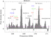 |
Fig. 1. NOEMA broadband (3.6 GHz) 2 mm spectrum of Mrk 231, centred on H2S. The x axis is rest frequency, and the y axis is flux in mJy. Identified lines have detection thresholds above 3σ (rms, indicated by the magenta line). |
List of molecular lines in the NOEMA band (Mrk 231).
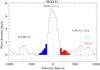 |
Fig. 2. NOEMA H2S spectrum of Mrk 231 (zoomed in from Fig. 1). The x axis is in km s−1 relative to the central velocity (12642 km s−1). Redshifted and blueshifted line-wing emission is indicated with corresponding colours. Other identified lines are indicated in the figure (same as in Fig. 1). |
NOEMA observation results for Mrk 231.
4. Discussion
This is the first survey of the λ = 2 mm 110–101 line of o-H2S in LIRGs. In this paper we report eight new detections, seven with APEX and one from NOEMA observations. To date, only three detections of 2 mm H2S line emission are reported outside our own galaxy: the Large Magellanic Cloud (LMC; e.g. Heikkilä et al. 1999), NGC 253 (e.g. Martin et al. 2005), and Arp 220 (e.g. Martín et al. 2011). Our sample, which is chosen from nearby LIRGs (see Sect. 2.1), includes a variety of galaxies in terms of morphology and kinematics.
4.1. H2S formation mechanisms
H2S can be formed through hydrogenation of a sulphur atom on grain surfaces, which can then be (i) thermally desorbed by shocks (Esplugues et al. 2014, Fig. 2) or by infrared radiation (e.g. Crockett et al. 2014), (ii) photodesorbed by UV radiation, (iii) desorbed after cosmic-ray impacts, or (iv) sputtered by shocks. Chemical desorption could be also efficient enough to release H2S into the gas phase (e.g. Oba et al. 2019; Navarro-Almaida et al. 2020), but it is not a dominant mechanism when we focus on starburst and AGN-host galaxies. Hydrogenation of sulphur is also possible in the gas phase if the kinetic temperature is higher than a few thousand kelvin (Mitchell 1984). For gas densities in excess of n = 104 cm−3, gas and dust are coupled and thermalised with similar temperatures. Therefore, under the assumption that most of the H2S emission is emerging from dense gas, the kinetic temperature of which can be between 10 to 300 K, hydrogenation in the gas phase is unlikely, because it is unlikely that the bulk of the dense gas can be maintained at such a high temperature. On smaller scales, close to heating sources, such high temperatures are, however, possible.
4.1.1. H2S enhancement via shocks
Shocks can cause both thermal desorption and mantle sputtering. For the case where the sulphur species are sputtered into the gas phase by strong shocks, Fig. 3 shows the average fractional abundance as a function of shock velocity for H2S (Holdship et al. 2017). In this figure, it can be seen that for low pre-shock gas densities (103 cm−3), the fractional abundance is 10−8 for shock velocities less than 20 km s−1, and increases by a factor of ∼100 for shock velocities > 30 km s−1. For higher pre-shock gas densities (> 104 cm−3), the abundance reaches values ∼10−6 even for shock velocities as low as ∼5 km s−1. This suggests that a high abundance of this molecule could be due to the passage of a shock in the absence of other mechanisms capable of releasing H2S from the ices. The caveat here is that this model considers only the case when most of the sulphur hydrogenates on the grains.
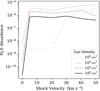 |
Fig. 3. Average fractional abundance as a function of shock velocity for H2S from Holdship et al. (2017). Each line shows a different pre-shock density; the log(nH) values are given in the lower-right plot. |
According to chemical models, H2S transforms quickly into SO, SO2, etc., within a timescale of ≤104 yr (e.g. Pineau des Forets et al. 1993). Shock elevation of H2S abundances therefore requires continuous replenishment, for example by internal shocks in the outflow. Internal shocks can occur if the molecular gas is interacting with hotter material in the outflow or if parts of the outflow is interacting with slower/faster moving gas components, for example due to periodic ejection processes. It is also possible that H2S is enhanced in highly turbulent gas. If so, the link to the outflow activity becomes less clear and may depend on whether the outflow process is feeding turbulence in the gas in a fountain scenario (e.g. Aalto et al. 2020). Other sources that drive turbulence include accretion and inflow, galactic rotation and stellar feedback (Klessen & Glover 2016).
4.1.2. H2S enhancement via thermal desorption, UV radiation, and cosmic rays
As discussed above, other possible methods for getting H2S off the grains and into the gas phase is by thermal desorption from warm grains, non-thermal UV photo-desorption, and cosmic-ray-induced desorption. In a recent Herschel study of higher rotationally excited H2S lines in the Orion hot core, Crockett et al. (2014) point to an H2S origin in dense, embedded gas, in close proximity to a hidden self-luminous protostellar source (i.e. heating the grains above the H2S sublimation temperature). In addition, Goicoechea et al. (2021) discuss and modell the photodesorption of H2S in UV-illuminated environment (PDRs) and this is a possible additional H2S formation mechanism for some of the sample galaxies. However, for some objects the gas and dust column densities will be too high to allow the UV radiation to penetrate very far. A further possible mechanism is cosmic-ray-induced desorption. These scenarios are further discussed in Sect. 4.4.
4.2. Column density and abundance
In this section we make simple estimates of column densities and abundances for basic comparisons with other sources and shock models. We assume collisional excitation for the H2S molecule throughout the paper (e.g. Mangum & Shirley 2015)4. H2S may also be pumped by infrared radiation, but Crockett et al. (2014) argued that infrared pumping for the transitions of H2S lower than J = 3 is unlikely because these transitions occur at longer wavelengths (λ > 100 μm).
Column densities of H2S, HCN, and HCO+ molecules for each galaxy were calculated using the formalism in Mangum & Shirley (2015, 2016, 2017). Since we have no direct information on the excitation of the H2S molecule nor the distribution of its emission, we have to make some assumptions to estimate the column densities. We have to assume an excitation temperature, Tex, and we estimated column densities for three different values of Tex of 30 K, 60 K, and 150 K to compare the results. This range of temperature is reflecting the span of kinetic temperature typically found in the inner regions of galaxies (e.g. Aalto et al. 1995; Mangum et al. 2013, 2019; Salak et al. 2014). This is often an upper limit to the excitation temperature. We also assumed a beam-filling factor of unity fs = 1 and optically thin (τ ≪ 1) emission for all lines for simplicity. We compare the H2S to the HCN abundance, assuming that both lines emerge from the same dense gas component and have the same Tex. The effect of these simplifying assumptions are to some extent cancelled out when we use the same assumption for all species and compare their ratios. For example, we find that the difference between resulting column density ratios for different Tex is small, less than a factor of two.
We consider the two most extreme cases in the observed H2S/HCN line ratios: NGC 4418 and NGC 1097 (see Table 5). We estimate the H2S/HCN abundance ratio (=column density ratio) to be X(H2S/HCN) ∼ 0.1 for NGC 4418 and ∼0.03 for NGC 1097 (for Tex = 60 K). We chose the column density values derived for an Tex of 60 K since it is an intermediate value for Tex. As noted above, the impact of the Tex on the column density ratio is quite small.
Integrated intensity ratios.
The difference in abundance ratio reflects the difference in the line intensity ratio between the two galaxies quite well. We therefore used the integrated intensity of H2S relative to HCN and HCO+ in Sects. 4.3 and 4.4 to indicate potential H2S enhancements in relation to the dense gas. The estimated values of X(H2S/HCN) seem reasonable compared to those found for the Galactic Orion star-forming complex. The value for X(H2S/HCN) varies strongly within the region, from < 10−4 in the ridge (quiescent gas) to ∼0.3 for the plateau (shocked gas) (Blake et al. 1987), while the X(H2S/HCN) for the Orion hot core may be greater than unity.
We also determined the H2S abundance in relation to H2 to X(H2S) ≈1.3 × 10⁻⁷ and X(H2S) ≈1.7 × 10⁻⁸ for NGC 4418 and NGC 1097, respectively. To obtain a value for N(H2), we obtained the molecular mass from the CO 1–0 luminosity5 assuming a standard CO-to-H2 conversion factor (Bolatto et al. 2013b). Assuming that the molecular mass was uniformly distributed in the APEX beam for our H2S observations we could calculate an average N(H2). Comparing to the shock model results presented in Fig. 3 shows that our simple estimation for X(H2S) is consistent with a shock origin of the observed H2S for NGC 4418. On the other hand, Crockett et al. (2014) show that these enhanced H2S abundances are caused by strong dust heating and subsequent thermal desorption in hot cores. In Sects. 4.3 and 4.4 we compare line ratios with dynamical and radiative properties of the galaxies to see if we can determine if outflows may be the cause behind H2S enhancements in LIRGs.
Our column density values are strongly affected by the assumptions on beam-filling factors and Tex. They give average values that, at best, are acceptable for searching for trends and correlations, but further high-resolution and multi-transition follow-up studies are required to chart the underlying causes behind H2S intensity enhancements. One example to illustrate this is NGC 4418. Costagliola et al. (2015) study the molecular excitation temperatures and column densities of many species in NGC 4418 with high-resolution and multi-transition observations using ALMA. They could compensate for the high optical depth of the HCN lines with a population diagram analysis, and (with an optically thin assumption for H2S) estimate X(H2S/HCN) ∼ 0.5. Should we use their local thermal equilibrium values, uncorrected for opacity, we would arrive at X(H2S/HCN) > 60. The discrepancy of this latter value compared to our result is that Costagliola et al. (2015) use a Tex of 7 K for HCN and 70 K for H2S, while we use the same value for both lines. HCN may also exist in more extended and colder region compared to H2S, which contributes to lowering the excitation.
4.3. Testing the notion of shock-enhanced H2S
Out of the 13 sample LIRGs, 10 have molecular outflows (see Table 1). In Sect. 4.1.1 we discussed a possible link between H2S enhancement and shocks in galaxies, for example caused by large-scale outflows. The sample galaxies display a range in outflow velocity, from slow (150 km s−1) to fast (> 250 km s−1).
To search for evidence of elevated H2S emission related to shock events, we put together line intensity ratios of H2S/HCO+ and H2S/HCN from our observation by APEX and NOEMA (see Table 5 and discussion in Sect. 4.2).
4.3.1. APEX single-dish data
We identify four galaxies with particularly elevated (a factor of two to three higher than in the rest of the sample) H2S/HCN ratios: Circinus, NGC 3256, NGC 4826 and NGC 4418. Of these, NGC 3256 has a fast molecular outflow (> 250 km s−1), Circinus and NGC 4418 have slow outflows (≈150 km s−1) while NGC 4826 has no report of a molecular outflow. Another example is the Seyfert galaxy NGC 1068, which has a striking AGN-driven molecular outflow (e.g. García-Burillo et al. 2014), but has a lower H2S/HCN ratio compared to NGC 4826, or M83 that lack known molecular outflows. In addition, both NGC 4945 and NGC 253 have slow molecular outflows with velocities of 50 km s−1, but their H2S line luminosity relative to HCN is quite different from each other (Table 5).
We find that the line ratios show considerable variation among our sample galaxies, but there is no apparent indication that H2S is more abundant in the galaxies with outflows, nor can we find any link to the outflow velocity. The lack of a clear link between the H2S/HCO+ and H2S/HCN line ratios and the presence, and properties, of an outflow could be because the link is not there, or because the large APEX beam (multi-kiloparsec scale) includes too much extended gas that is unconnected to the outflow. Indeed, H2S absorption has been detected even in diffuse clouds (Lucas & Liszt 2002), which may also contribute and dilute our results. Furthermore, the single-dish data lack the sensitivity and stability necessary to compare the relative H2S enhancement in the line core to that in the line wings.
Therefore, it is important to investigate potential enhancements of H2S in outflows with high-resolution observations, both spectroscopically and spatially, for a sample of galaxies.
4.3.2. Mrk 231 with NOEMA
To search for indications of shock chemistry in an outflow with higher spatial resolution, we observed the 168 GHz ground-state H2S line with the NOEMA telescope towards Mrk 231.
The ULIRG quasar Mrk 231 has an extremely strong and fast molecular outflow where CO has been detected out to velocities of 750 km s−1 (Feruglio et al. 2010). The molecular outflow also shows remarkably luminous HCN emission, which is suggested to be caused by large masses of dense molecular gas, but also by elevated HCN abundances (Aalto 2012; Aalto et al. 2015b). It is suggested that the HCN enhancement is caused by the molecular gas being compressed and fragmented by shocks in the outflow.
We detected the H2S line with a peak intensity of ≈7.2 mJy (Fig. 2) and the line has wings at both sides indicating H2S emission in the outflow at least out to velocities of −300 km s−1 and +500 km s−1 (see Sect. 3.2). However, when we compare the relative intensity of the H2S emission to that of HCN 2–1, we see no sign of an elevated H2S intensity in the line wings with respect to the core. Therefore, the relatively faint H2S emission appears inconsistent with the notion of dominant shock chemistry in the molecular outflow of Mrk 231. More studies of the molecular formation and destruction processes of the Mrk 231 are necessary (see for example the recent detection of CN in the outflow by Cicone et al. 2020).
It is interesting to compare Mrk 231 to the H2S-luminous merger LIRG NGC 3256. This galaxy exhibits two strong and fast outflows: one from each nucleus (e.g. Sakamoto et al. 2014). NGC 3256 has a distinct H2S enhancement in relation to HCN and we require high-resolution observations to determine if the enhancement is linked to any, or both, of the two outflows, or to some other part of its molecular emission.
4.4. H2S enhancement caused by thermal desorption: The ‘hot-core-like’ nuclear obscuration of NGC 4418
H2S enhancements may also be caused by other processes such as thermal desorption (see Sect. 4.1.2). For example, in a high-resolution study of H2S towards NGC 253, Minh et al. (2007) argue that H2S enhancements might be associated with young massive star formation, which may imply a scenario of radiative thermal desorption.
NGC 4418 and IC 860 are suggested to host so-called compact obscured nuclei (CONs) in their central regions (e.g. Costagliola et al. 2011, 2013; Sakamoto et al. 2013; Falstad et al. 2019; Aalto et al. 2019). A CON is a region of exceptionally high H2 column density (N(H2) > 1025 cm−2) and with very high infrared luminosity surface brightness and gas temperatures (in excess of 200 K). Studies of IC 860 also find that the gas densities can be high with n ∼ 107 cm−3 (Aalto et al. 2019).
Methyl cyanide CH3CN, known as a tracer of dense and warm gas (e.g. Churchwell & Hollis 1983), was detected in IC 860, NGC 4418, NGC 253, and NGC 4945. The line luminosity of CH3CN 9-8 shows at least an order of magnitude higher values for NGC 4418 (LCH3OH = 1.66 × 10⁵ L⊙) and IC 860 (2.37 × 10⁵ L⊙) than for NGC 253 (6.36 × 10³ L⊙) and NGC 4945 (2.52 × 10⁴ L⊙).
It seems likely that the CH3CN emission is enhanced because of the high density and temperature in the CONs. The luminous CH3CN emission in NGC 4418 may imply that the H2S enhancement here is caused by desorption driven by radiation (Sect. 4.1.2), for example through UV radiation from a buried source. However, NGC 4418 has an extremely large H2 column density with N(H2) > 1025 cm−2 (Costagliola et al. 2013; Sakamoto et al. 2013). Since UV photons cannot penetrate long distances through such a high column density region, the global H2S enhancement is unlikely to be caused by photodesorption by UV radiation. In addition, Bayet et al. (2009) argued that H2S is unlikely to trace gas in PDRs in starburst galaxies, or near AGN.
Alternatively, high energy photons and particles can pass through high column density cores and may photo- or thermally desorb H2S out from grain surface over wider regions. Observations with the Chandra X-ray satellite by Maiolino et al. (2003) do not show a clear X-ray signature in NGC 4418. The extreme column densities of NGC 4418 are difficult to penetrate completely for X-rays. However, the X-rays reach further than UV and it is possible that they may impact the nuclear chemistry and provide large bulk gas temperatures that can result in an H2S enhancement. González-Alfonso et al. (2013) proposed that X-ray ionisation due to an AGN is responsible for the molecular ion chemistry in the centre of NGC 4418.
Of the four LIRGs that have elevated H2S/HCN intensity ratios, one does not show any evidence of either a molecular outflow or a ‘hot core’: NGC 4826. This galaxy shows strong evidence of counter-rotating gas and stars, and its inner 1 kpc shows the signatures of different types of m = 1 perturbations (such as streaming motions) in the gas (García-Burillo et al. 2003). A possibility is that the perturbations drive turbulence that may also lead to H2S enhancements (Sect. 4.1.1).
4.5. Mass outflow rates and the global dense gas properties
In Sect. 4.3.1 we find no link between global H2S abundance enhancements in the dense gas, and the presence (or velocity) of an outflow. There appears to be no general process that leads to significant H2S abundance enhancements within the outflows, or when outflows are impacting their host galaxies. (Although enhancements are still possible on smaller scales that are diluted in our single-dish beam.)
However, to understand the launch mechanism and outflow evolution, it is also important to study and compare other molecular properties of the host galaxy to that of its outflow. A correlation between the outflow mass or its velocity with, for example, the molecular gas mass or dense gas content of the host galaxy gives essential clues to the origin of the molecular gas in the outflow.
To search for such host galaxy-outflow relations, we investigate correlations between the global line luminosity of H2S, HCN, and HCO+ and the mass of the global molecular gas for our sample galaxies and the velocities and molecular masses of their outflows (Fluetsch et al. 2019, Table 2). The galaxies that are in our sample and also have their outflow information are Circinus, NGC 3256, NGC 1068, NGC 253, NGC 4418, and Mrk 231.
We find a correlation between L(H2S) and the molecular mass, Moutflow(H2), of the outflow (Fig. 4), where L(H2S) is highest for the galaxies with the highest Moutflow(H2). This could be because L(H2S) is a rough probe of the host galaxy molecular mass and that the two are connected, that is, that the ejected molecular gas mass is directly drawn from the large-scale molecular reservoir of the galaxy. This notion can be tested through investigating the correlation between Moutflow and other tracers of host galaxy molecular mass, such as the CO 1–0 luminosity, L(CO).
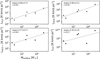 |
Fig. 4. Line luminosities of H2S 2–1 (top left), HCN 2–1 (top right), HCO+ 2–1 (lower left), and CO 1–0 (lower right) of Circinus, NGC 3256, NGC 1068, NGC 253, NGC 4418, and Mrk 231, plotted against the molecular mass of the outflow, Moutflow, taken from Fluetsch et al. (2019). The correlation coefficient between the line luminosity and Mout is given in the upper-left corner of each panel, as is the slope of the line. |
We use global CO 1–0 luminosities (Sanders et al. 1991; Planesas et al. 1989; Aalto et al. 1995; Elmouttie et al. 1998; Houghton et al. 1997) for our sample galaxies and find that L(CO) correlates more poorly with Moutflow(H2) than L(H2S): the correlation coefficient is r = 0.93 for H2S and r = 0.57 for CO. The corresponding correlation coefficients for L(HCN) and L(HCO+) are r = 0.91 and r = 0.83, respectively. If we compare the critical densities, ncrit, of the observed transitions, we find that H2S and HCN have the highest ncrit followed by HCO+ while the 1–0 transition of CO has an ncrit several orders of magnitude lower. The molecular mass in the outflow appears to be more strongly connected to the dense gas (traced by H2S and HCN) in the host galaxy, rather than the total available molecular reservoir. We note that this suggested correlation between H2S (and HCN) and the outflow mass is different from the lack of correlation between H2S abundances and outflow properties discussed in Sect. 4.3. Here we use H2S as a probe of the densest molecular gas, instead of searching for enhancements in the H2S abundances as an effect of the outflow.
Since the correlations are found for the relatively limited number of sources in our sample, we decided to search for HCN data in the literature to test the notion that Moutflow(H2) is more strongly correlated with the dense gas tracers than CO 1–0. We found HCN 1–0 data for 24 galaxies in the Fluetsch et al. (2019) sample (listed in Table 6). HCN 1–0 has a lower critical density than the 2–1 transition and we expect to see a lower correlation coefficient with Moutflow(H2) than for HCN 2–1, which we also find with a value of r = 0.68 (Fig. 5). Fluetsch et al. (2019) also lists values for M(H2) for their sample outflow host galaxies. Using these values for the 24 galaxies for which we have HCN 1–0 information, we find a correlation coefficient between M(H2) and Moutflow(H2) of r = 0.25. This is significantly lower than what we find for L(CO) for our sample galaxies (Fig. 4). This may be because the molecular masses listed in Fluetsch et al. (2019) are not global, masses, or because the correlation between Moutflow(H2) and the total reservoir becomes even poorer in large samples.
HCN 1–0 data from the literature.
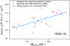 |
Fig. 5. Same plot as Fig. 4 but for the luminosities of HCN 1–0. The values for the molecular mass of the outflow, Moutflow, are from Fluetsch et al. (2019). The LHCN1−0 values are from the references in Table 6. AGN-powered outflows are indicated with the red ‘x’ symbol. |
A possible interpretation is that the molecular mass in the outflow is linked to the properties and mass of the most centrally concentrated gas, traced by HCN and H2S. This is expected if the outflows are launched from the inner regions of galaxies. In addition, it is also compatible with the scenario where the gas is being ejected from the host galaxy in molecular form, through entrainment by jets and winds, a molecular magneto-hydrodynamic wind, or by radiation pressure (e.g. Veilleux et al. 2013). It appears less consistent with the notion that the molecular gas is primarily formed in the outflows themselves through instabilities in the hot gas (e.g. Zubovas & King 2014; Ferrara & Scannapieco 2016).
Lutz et al. (2020) find a correlation between bolometric luminosity, L(bol), and Moutflow(H2), with similar relations that we find between L(HCN) and Moutflow(H2). They also find that the AGN luminosity, L(AGN), correlates with Moutflow(H2) for objects with L(AGN) > 1010 L⊙. Lutz et al. (2020) point out that L(bol) is linked to both AGN activity and star formation, making the relation to L(bol) somewhat difficult to interpret, but that AGN activity plays and important role in outflow driving. We note that the link between L(HCN) and Moutflow(H2) is stronger for the objects that Fluetsch et al. (2019) identify as AGN powered (see Fig. 5).
The correlation between Moutflow and luminosity of dense gas tracers in the host galaxy should be tested on larger samples. Furthermore, high-resolution imaging is required to test the notion of a higher degree of central concentration for H2S and HCN and to what degree this emission is linked to the launch regions of outflows.
4.6. H2S and H2O
Because of their chemical similarity, H2S and H2O have similar formation processes, including regarding the grain chemistry: both molecules may go through thermal or photo (non-thermal) desorption by shock or radiation. Although the more volatile H2S will leave the grains at lower temperatures than more tightly bound H2O (Rodgers & Charnley 2003). The discussion below is based on two assumptions: (1) sulphur hydrogenates in H2S on the dust grains, which is still debated, and (2) H2S does not get dissociated when it is desorbed, even though Oba et al. (2019) show it actually does. Due to the similarities, it is conceivable that H2S may serve as a water proxy, with its ground-state line accessible by ground-based telescopes for nearby galaxies. In this case, we would expect a correlation between the H2O and H2S properties of our sample galaxies and open up the possibility to use H2S as an initial substitute in searches for water in nearby galaxies.
Yang et al. (2013) fit several transition of water emission luminosities against the corresponding LIR (see Yang et al. 2013, Fig. 1 and Table 1). The fit can be described as
 (1)
(1)
They report the results for eight transitions and the factor α varied between 0.78 and 1.21. For the ground-state (para) H2O line they find a α = 0.89 ± 0.09 (using χ2 fitting). We carried out the same fitting for H2S and HCN. The line luminosities were calculated using the formula ![Mathematical equation: $ L_{\mathrm{line}} [L_{\odot}] = 1.04 \times 10^{-3} \times S_{\mathrm{line}} \Delta \mathit{v} D^{2}_{\mathrm{L}} \times \nu_{\mathrm{obs}} $](/articles/aa/full_html/2022/04/aa41260-21/aa41260-21-eq13.gif) , where SlineΔv is the measured flux of the line [Jy km s−1], DL is the luminosity distance [Mpc] and νobs is the frequency of the line [GHz]. I[Jy km s−1] = I[K km s−1] × 40.67 [Jy K−1] is used to calculate the line flux from the observed antenna temperature (Carilli & Walter 2013)6. In Fig. 6 we show plots of the line luminosity of H2S and HCN versus the infrared luminosity of each galaxy.
, where SlineΔv is the measured flux of the line [Jy km s−1], DL is the luminosity distance [Mpc] and νobs is the frequency of the line [GHz]. I[Jy km s−1] = I[K km s−1] × 40.67 [Jy K−1] is used to calculate the line flux from the observed antenna temperature (Carilli & Walter 2013)6. In Fig. 6 we show plots of the line luminosity of H2S and HCN versus the infrared luminosity of each galaxy.
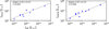 |
Fig. 6. Line luminosity of H2S (left) and HCN (right) versus the infrared luminosity of each sample galaxy in which the H2S line is detected. The correlation coefficient and the slope of the fitting line are given in the upper-left corner of each panel. |
We find a factor α (in Eq. (1)) of 1.01 ± 0.12 (χ2) for H2S and 1.07 ± 0.12 (χ2) for HCN. This is within the error of the value found for the ground-state H2O line. Yang et al. (2013) suggest that the reason that the correlation between H2O and infrared is near-linear is infrared pumping of the H2O lines. They argue that, after absorbing a far-infrared photon, the upper levels cascade down to populate lower levels in a constant fraction, yielding a linear relationship with LIR, and that the linear correlation shows the importance of infrared pumping. Although it is true that infrared pumping is important for the excitation of H2O it is not clear that the same logic can be applied to the near-linear correlations found for H2S and HCN. Crockett et al. (2014) claim that infrared pumping of H2S for transitions lower than J = 3 is not possible. The near-linear correlation between LHCN and LIR (first reported for LIRGs by Gao & Solomon 2004) is also not clearly connected to infrared pumping, even if the HCN rotational ladder can be pumped via a mid-infrared bending mode (e.g. Aalto et al. 1994). Gao & Solomon (2004) argue that the HCN-infrared correlation is due to HCN probing dense gas engaged in star formation, which in turn gives rise to the infrared luminosity. We conclude that H2S, H2O, and HCN seem to correlate in a similar way with LIR, which may indicate that they emerge from similar regions in the LIRGs.
5. Conclusions
Using the APEX telescope, we observed the λ = 2 mm 110–101 line of ortho-H2S towards the centres of 12 nearby luminous galaxies and detected H2S emission in nine of them. We also detected HCN and HCO+ 2–1 in 11 of the sample galaxies as well as HNC, SO, CH3OH, CH3CN, H2CS, and HOC+ in some galaxies. In addition, we observed H2S in the ULIRG Mrk 231 with the NOEMA telescope. Our aim was to study the impact of outflows on the chemistry and physical conditions of the gas in the host galaxy and outflow using H2S as a potential tracer of the impact of shocks. The line intensity ratio of H2S to HCN (and to HCO+) shows considerable variation, which could be due to significant differences in H2S abundance among the studied galaxies. Four galaxies stand out as particularly H2S luminous: two exhibit strong outflows, one harbours a CON, and one shows evidence of gas and star counter-rotation possibly feeding turbulence. These results support previous suggestions that the H2S emission may become enhanced in both shocked and irradiated dusty gas in the centres of luminous, gas-rich galaxies. However, for the sample galaxies as a whole, we find no correlation between the H2S/HCN or the H2S/HCO+ line ratios with the presence of a molecular outflow or its speed. In Mrk 231 we detect H2S out to −300 and +500 km s−1, but the emission is not enhanced with respect to that of HCN. The relatively faint H2S emission in the line wings appears inconsistent with the notion of shock chemistry in the molecular outflow of Mrk 231.
We also investigated other possible connections between host galaxy molecular properties and those of their outflows. We found no link between the luminosities of H2S 110–101, HCN 2–1, HCO+2–1, or CO 1–0 with the outflow velocity. In contrast, we did find a correlation with the molecular mass of the outflow, Moutflow(H2), where the correlation coefficient is strongest for LH2S and LHCN and weakest for LCO. We suggest that LH2S serves as a tracer of the dense gas content, similar to LHCN, and that the correlation between LH2S and Moutflow(H2) implies a relation between the dense gas reservoir and the properties and evolution of the molecular feedback. The dense gas component is likely more centrally concentrated than the bulk of the molecular gas (traced by CO 1–0), and a possible explanation is that the outflows are launched in the central regions and that the molecular gas in the outflow stems from the reservoir in the inner region, rather than being formed from instabilities in the hot gas. However, further studies of this correlation are needed to understand its cause. In addition, it is important to mention that the enhancement of H2S could also be related to starburst regions dominated by dense molecular gas and UV radiation.
Finally, based on the chemical similarities between H2S and H2O, we studied whether the two species show analogous behaviour in how they correlate to the infrared luminosity. We find that their infrared-correlation coefficients are similar, which could indicate that they originate in the same regions in the galaxy: warm gas in shocks or irradiated by star formation or an AGN.
See http://www.iram.fr/IRAMFR/GILDAS for more information about the GILDAS software.
ncrit, H2S ≈ 7.8 × 10⁵[cm−3], ncrit, HCN(2−1) ≈ 1.3 × 10⁷[cm−3], ncrit, HCO+(2−1) ≈ 1.2 × 10⁶[cm−3] and ncrit, CO(1−0) ≈ 2.2 × 10³ [cm−3] at Tk = 30 K. See Appendix C.
CO 1–0 luminosities taken from Sanders et al. (1991) for NGC 4418 and Gerin et al. (1988) for NGC 1097.
Acknowledgments
We thank the anonymous referee for the constructive comments and suggestions which improved the manuscript. Based on observations with the Atacama Pathfinder EXperiment (APEX) telescope under project numbers 096.F-9331(A), 099.F-9312(A) and 0100.F-9311(A). APEX is a collaboration between the Max Planck Institute for Radio Astronomy, the European Southern Observatory, and the Onsala Space Observatory. Swedish observations on APEX are supported through Swedish Research Council grant No 2017-00648. Based on observations carried out under project number W16BW with the IRAM NOEMA Interferometer. IRAM is supported by INSU/CNRS (France), MPG (Germany) and IGN (Spain). M.S., S.A. and S.K. gratefully acknowledge funding from the European Research Council (ERC) under the European Union’s Horizon 2020 research and innovation programme (grant agreement No 789410) SV acknowledges the European Research Council (ERC) Advanced Grant MOPPEX 833460. YN is supported by NAOJ ALMA Scientific Research grant No. 2017-06B and JSPS KAKENHI grant No. JP18K13577. KK acknowledges the support by JSPS KAKENHI grant No. JP17H06130.
References
- Aalto, S. 2012, Proc. Int. Astron. Union, 8, 199 [NASA ADS] [CrossRef] [Google Scholar]
- Aalto, S., Booth, R. S., Black, J. H., Koribalski, B., & Wielebinski, R. 1994, A&A, 286, 365 [Google Scholar]
- Aalto, S., Booth, R. S., Black, J. H., & Johansson, L. E. 1995, A&A, 300, 369 [NASA ADS] [Google Scholar]
- Aalto, S., Garcia-Burillo, S., Muller, S., et al. 2012, A&A, 537, A44 [NASA ADS] [CrossRef] [EDP Sciences] [Google Scholar]
- Aalto, S., Garcia-Burillo, S., Muller, S., et al. 2015a, A&A, 574, A85 [NASA ADS] [CrossRef] [EDP Sciences] [Google Scholar]
- Aalto, S., Martin, S., Costagliola, F., et al. 2015b, A&A, 584, A42 [NASA ADS] [CrossRef] [EDP Sciences] [Google Scholar]
- Aalto, S., Costagliola, F., Muller, S., et al. 2016, A&A, 590, A73 [NASA ADS] [CrossRef] [EDP Sciences] [Google Scholar]
- Aalto, S., Muller, S., König, S., et al. 2019, A&A, 627, A147 [NASA ADS] [CrossRef] [EDP Sciences] [Google Scholar]
- Aalto, S., Falstad, N., Muller, S., et al. 2020, A&A, 640, A104 [EDP Sciences] [Google Scholar]
- Barbosa, F. K. B., Storchi-Bergmann, T., Mcgregor, P., Vale, T. B., & Rogemar Riffel, A. 2014, MNRAS, 445, 2353 [NASA ADS] [CrossRef] [Google Scholar]
- Barcos-Muñoz, L., Aalto, S., Thompson, T. A., et al. 2018, ApJ, 853, L28 [Google Scholar]
- Bayet, E., Viti, S., Williams, D. A., Rawlings, J. M., & Bell, T. 2009, ApJ, 696, 1466 [NASA ADS] [CrossRef] [Google Scholar]
- Blake, G. A., Sutton, E. C., Masson, C. R., & Phillips, T. G. 1987, ApJ, 315, 621 [Google Scholar]
- Bolatto, A. D., Warren, S. R., Leroy, A. K., et al. 2013a, Nature, 499, 450 [Google Scholar]
- Bolatto, A. D., Wolfire, M., & Leroy, A. K. 2013b, ARA&A, 51, 207 [CrossRef] [Google Scholar]
- Brauher, J. R., Dale, D. A., & Helou, G. 2008, ApJS, 178, 280 [NASA ADS] [CrossRef] [Google Scholar]
- Carilli, C., & Walter, F. 2013, ARA&A, 51, 105 [NASA ADS] [CrossRef] [Google Scholar]
- Charnley, S. B. 1997, ApJ, 481, 396 [NASA ADS] [CrossRef] [Google Scholar]
- Chung, A., Yun, M. S., Naraynan, G., Heyer, M., & Erickson, N. R. 2011, ApJ, 732, 1 [Google Scholar]
- Churchwell, E., & Hollis, J. 1983, ApJ, 272, 591 [NASA ADS] [CrossRef] [Google Scholar]
- Cicone, C., Maiolino, R., Sturm, E., et al. 2014, A&A, 562, A21 [NASA ADS] [CrossRef] [EDP Sciences] [Google Scholar]
- Cicone, C., Maiolino, R., Aalto, S., Muller, S., & Feruglio, C. 2020, A&A, 633, A163 [NASA ADS] [CrossRef] [EDP Sciences] [Google Scholar]
- Contini, T., Wozniak, H., Considère, S., & Davoust, E. 1997, A&A, 324, 41 [NASA ADS] [Google Scholar]
- Costagliola, F., Aalto, S., Rodriguez, M. I., et al. 2011, A&A, 528, A30 [NASA ADS] [CrossRef] [EDP Sciences] [Google Scholar]
- Costagliola, F., Aalto, S., Sakamoto, K., et al. 2013, A&A, 556, A66 [NASA ADS] [CrossRef] [EDP Sciences] [Google Scholar]
- Costagliola, F., Sakamoto, K., Muller, S., et al. 2015, A&A, 582, A91 [NASA ADS] [CrossRef] [EDP Sciences] [Google Scholar]
- Crockett, N. R., Bergin, E. A., Neill, J. L., et al. 2014, ApJ, 781, 114 [NASA ADS] [CrossRef] [Google Scholar]
- Curran, S. J., Rydbeck, G., Johansson, L. E. B., & Booth, R. S. 1999, A&A, 778, 767 [Google Scholar]
- Dasyra, K. M., Combes, F., Oosterloo, T., et al. 2016, A&A, 595, L7 [NASA ADS] [CrossRef] [EDP Sciences] [Google Scholar]
- Elmouttie, M., Krause, M., Haynes, R. F., & Jones, K. L. 1998, MNRAS, 300, 1119 [NASA ADS] [CrossRef] [Google Scholar]
- Emsellem, E., Fathi, K., Wozniak, H., et al. 2006, MNRAS, 365, 367 [Google Scholar]
- Esplugues, G. B., Viti, S., Goicoechea, J. R., & Cernicharo, J. 2014, A&A, 567, A1 [Google Scholar]
- Evans, A., Solomon, P., Tacconi, L., Vavilkin, T., & Downes, D. 2006, AJ, 132, 2398 [NASA ADS] [CrossRef] [Google Scholar]
- Falstad, N., Hallqvist, F., Aalto, S., et al. 2019, A&A, 623, A79 [NASA ADS] [CrossRef] [EDP Sciences] [Google Scholar]
- Ferrara, A., & Scannapieco, E. 2016, ApJ, 833, 46 [NASA ADS] [CrossRef] [Google Scholar]
- Feruglio, C., Maiolino, R., Piconcelli, E., et al. 2010, A&A, 518, L155 [NASA ADS] [CrossRef] [EDP Sciences] [Google Scholar]
- Feruglio, C., Daddi, E., Fiore, F., et al. 2011, ApJ, 729, 2 [Google Scholar]
- Fluetsch, A., Maiolino, R., Carniani, S., et al. 2019, MNRAS, 483, 4586 [NASA ADS] [Google Scholar]
- Gao, Y., & Solomon, P. M. 2004, ApJ, 606, 271 [NASA ADS] [CrossRef] [Google Scholar]
- García-Burillo, S., Combes, F., Hunt, L. K., et al. 2003, A&A, 407, 485 [NASA ADS] [CrossRef] [EDP Sciences] [Google Scholar]
- García-Burillo, S., Combes, F., Usero, A., et al. 2014, A&A, 567, A125 [Google Scholar]
- García-Burillo, S., Combes, F., Usero, A., et al. 2015, A&A, 580, A35 [Google Scholar]
- Gerin, M., Nakai, N., & Combes, F. 1988, A&A, 203, 44 [NASA ADS] [Google Scholar]
- Goicoechea, J. R., Aguado, A., Cuadrado, S., et al. 2021, A&A, 647, A10 [EDP Sciences] [Google Scholar]
- González-Alfonso, E., Fischer, J., Isaak, K., et al. 2010, A&A, 518, L43 [NASA ADS] [CrossRef] [EDP Sciences] [Google Scholar]
- González-Alfonso, E., Fischer, J., Graciá-Carpio, J., et al. 2012, A&A, 541, A4 [NASA ADS] [CrossRef] [EDP Sciences] [Google Scholar]
- González-Alfonso, E., Fischer, J., Bruderer, S., et al. 2013, A&A, 550, A25 [NASA ADS] [CrossRef] [EDP Sciences] [Google Scholar]
- Gracia-Carpio, J., Garcia-Burillo, S., Planesas, P., & Colina, L. 2006, ApJ, 640, 135 [Google Scholar]
- Heikkilä, A., Johansson, L. E., & Olofsson, H. 1999, A&A, 344, 817 [Google Scholar]
- Henkel, C., Mühle, S., Bendo, G., et al. 2018, A&A, 615, A155 [NASA ADS] [CrossRef] [EDP Sciences] [Google Scholar]
- Holdship, J., Viti, S., Makrymallis, A., & Priestley, F. 2017, AJ, 154, 38 [NASA ADS] [CrossRef] [Google Scholar]
- Houghton, S., Whiteoak, J. B., Koribalski, B., et al. 1997, A&A, 325, 923 [NASA ADS] [Google Scholar]
- Huang, Y., Zhang, J. S., Liu, W., & Xu, J. 2018, J. Astrophys. Astron., 39, 34 [NASA ADS] [CrossRef] [Google Scholar]
- Imanishi, M., Nakanishi, K., Tamura, Y., Oi, N., & Kohno, K. 2007, AJ, 134, 2366 [NASA ADS] [CrossRef] [Google Scholar]
- Iono, D., Wilson, C. D., Yun, M. S., et al. 2009, ApJ, 695, 1537 [NASA ADS] [CrossRef] [Google Scholar]
- Israel, F. P., Güsten, R., Meijerink, R., Requena-Torres, M. A., & Stutzki, J. 2017, A&A, 599, A53 [NASA ADS] [CrossRef] [EDP Sciences] [Google Scholar]
- Klessen, R. S., & Glover, S. C. O. 2016, Saas-Fee Adv. Course, 43, 85 [NASA ADS] [CrossRef] [Google Scholar]
- Lindberg, J. E., Aalto, S., Muller, S., et al. 2016, A&A, 587, A15 [NASA ADS] [CrossRef] [EDP Sciences] [Google Scholar]
- Lucas, R., & Liszt, H. S. 2002, A&A, 384, 1054 [NASA ADS] [CrossRef] [EDP Sciences] [Google Scholar]
- Lutz, D., Sturm, E., Janssen, A., et al. 2020, A&A, 633, A134 [NASA ADS] [CrossRef] [EDP Sciences] [Google Scholar]
- Maiolino, R., Comastri, A., Gilli, R., et al. 2003, MNRAS, 344, L59 [NASA ADS] [CrossRef] [Google Scholar]
- Maiolino, R., Russell, H. R., Fabian, A. C., et al. 2017, Nature, 544, 202 [Google Scholar]
- Mangum, J. G., & Shirley, Y. L. 2015, PASP, 127, 266 [Google Scholar]
- Mangum, J. G., & Shirley, Y. L. 2016, PASP, 128, L029201 [NASA ADS] [Google Scholar]
- Mangum, J. G., & Shirley, Y. L. 2017, PASP, 129, L069201 [NASA ADS] [CrossRef] [Google Scholar]
- Mangum, J. G., Darling, J., Henkel, C., et al. 2013, ApJ, 779, 108 [NASA ADS] [CrossRef] [Google Scholar]
- Mangum, J. G., Ginsburg, A. G., Henkel, C., et al. 2019, ApJ, 871, 170 [NASA ADS] [CrossRef] [Google Scholar]
- Martín, S., Krips, M., Aalto, S., et al. 2011, A&A, 527, A36 [NASA ADS] [CrossRef] [EDP Sciences] [Google Scholar]
- Martin, S., Martin-Pintado, J., Mauersberger, R., Henkel, C., & Garcia-Burillo, S. 2005, ApJ, 620, 210 [CrossRef] [Google Scholar]
- Matsushita, S., Trung, D.-V., Boone, F., et al. 2015, Publ. Korean Astron. Soc., 30, 439 [Google Scholar]
- Michiyama, T., Iono, D., Sliwa, K., et al. 2018, ApJ, 868, 95 [Google Scholar]
- Minh, Y. C., Irvine, W. M., McGonagle, D., & Ziurys, L. M. 1990, ApJ, 360, 136 [NASA ADS] [CrossRef] [Google Scholar]
- Minh, Y. C., Muller, S., Liu, S.-Y., & Yoon, T. S. 2007, ApJ, 661, L135 [NASA ADS] [CrossRef] [Google Scholar]
- Mitchell, G. F. 1984, ApJ, 287, 665 [NASA ADS] [CrossRef] [Google Scholar]
- Morganti, R., Oosterloo, T., Raymond Oonk, J. B., Frieswijk, W., & Tadhunter, C. 2015, A&A, 580, A1 [NASA ADS] [CrossRef] [EDP Sciences] [Google Scholar]
- Navarro-Almaida, D., Gal, R. L., Fuente, A., et al. 2020, A&A, 637, A39 [NASA ADS] [CrossRef] [EDP Sciences] [Google Scholar]
- Nishimura, Y., Watanabe, Y., Harada, N., et al. 2017, ApJ, 848, 17 [NASA ADS] [CrossRef] [Google Scholar]
- Oba, Y., Tomaru, T., Kouchi, A., & Watanabe, N. 2019, ApJ, 874, 124 [NASA ADS] [CrossRef] [Google Scholar]
- Ohyama, Y., Sakamoto, K., Aalto, S., & Gallagher, J. S. 2019, ApJ, 871, 191 [NASA ADS] [CrossRef] [Google Scholar]
- Pereira-Santaella, M., Colina, L., García-Burillo, S., et al. 2018, A&A, 616, A171 [NASA ADS] [CrossRef] [EDP Sciences] [Google Scholar]
- Pineau des Forets, G., Roueff, E., Schilke, P., & Flower, D. R. 1993, MNRAS, 262, 915 [CrossRef] [Google Scholar]
- Planesas, P., Gómez-González, J., & Martín-Pintado, J. 1989, A&A, 216, 1 [NASA ADS] [Google Scholar]
- Privon, G. C., Herrero-Illana, R., Evans, A. S., et al. 2015, ApJ, 814, 39 [CrossRef] [Google Scholar]
- Rodgers, S. D., & Charnley, S. B. 2003, ApJ, 585, 355 [NASA ADS] [CrossRef] [Google Scholar]
- Sakamoto, K., Aalto, S., Costagliola, F., et al. 2013, ApJ, 764, 42 [Google Scholar]
- Sakamoto, K., Aalto, S., Combes, F., Evans, A., & Peck, A. 2014, ApJ, 797, 90 [Google Scholar]
- Sakamoto, K., Aalto, S., Barcos-Muñoz, L., et al. 2017, ApJ, 849, 14 [Google Scholar]
- Salak, D., Nakai, N., & Kitamoto, S. 2014, PASJ, 66, 1 [NASA ADS] [CrossRef] [Google Scholar]
- Sanders, D. B., & Mirabel, I. F. 1996, ARA&A, 34, 749 [Google Scholar]
- Sanders, D. B., Scoville, N. Z., & Soifer, B. T. 1991, ApJ, 370, 158 [NASA ADS] [CrossRef] [Google Scholar]
- Sanders, D. B., Mazzarella, J. M., Kim, D.-C., Surace, J. A., & Soifer, B. T. 2003, AJ, 126, 1607 [Google Scholar]
- Shirley, Y. L. 2015, PASP, 127, 299 [Google Scholar]
- Spoon, H. W., Farrah, D., Lebouteiller, V., et al. 2013, ApJ, 775, 127 [NASA ADS] [CrossRef] [Google Scholar]
- Sturm, E., Gonzlez-Alfonso, E., Veilleux, S., et al. 2011, ApJ, 733, L16 [NASA ADS] [CrossRef] [Google Scholar]
- Veilleux, S., Meléndez, M., Sturm, E., et al. 2013, ApJ, 776, 21 [NASA ADS] [CrossRef] [Google Scholar]
- Veilleux, S., Maiolino, R., Bolatto, A. D., & Aalto, S. 2020, A&ARv, 28, 2 [NASA ADS] [CrossRef] [Google Scholar]
- Viti, S., Collings, M. P., Dever, J. W., McCoustra, M. R., & Williams, D. A. 2004, MNRAS, 354, 1141 [NASA ADS] [CrossRef] [Google Scholar]
- Wakelam, V., Castets, A., Ceccarelli, C., et al. 2004, A&A, 413, 609 [NASA ADS] [CrossRef] [EDP Sciences] [Google Scholar]
- Walter, F., Bolatto, A. D., Leroy, A. K., et al. 2017, ApJ, 835, 265 [NASA ADS] [CrossRef] [Google Scholar]
- Woods, P. M., Occhiogrosso, A., Viti, S., et al. 2015, MNRAS, 450, 1256 [Google Scholar]
- Yang, C., Gao, Y., Omont, A., et al. 2013, ApJ, 771, L29 [NASA ADS] [CrossRef] [Google Scholar]
- Zschaechner, L. K., Walter, F., Bolatto, A., et al. 2016, ApJ, 832, 1 [CrossRef] [Google Scholar]
- Zubovas, K., & King, A. R. 2014, MNRAS, 439, 400 [Google Scholar]
Appendix A: Spectra of the APEX sample galaxies
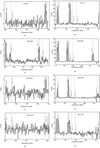 |
Fig. A.1. Spectra taken with SEPIA. The intensity scale is in T |

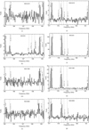 |
Fig. A.1. Continued. |
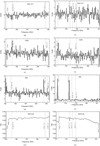 |
Fig. A.1. Continued. |
Appendix B: APEX results
APEX results.
Appendix C: Notes on critical densities
In this paper the critical densities of H2S, HCN, and HCO+ were calculated assuming the molecules are two-level systems,
 (C.1)
(C.1)
where Aul is the spontaneous transition probability of the transition u to l and qul is the corresponding collisional rate coefficient. This simple approach is sufficient for the comparison of critical densities in Sect. 4.2.
A more realistic estimate of the critical density is
 (C.2)
(C.2)
where one allows for transitions between more levels. In general it gives lower values. Furthermore, opacity will also impact the critical density (for further discussion, see for example Shirley 2015).
All Tables
All Figures
|
Fig. 1. NOEMA broadband (3.6 GHz) 2 mm spectrum of Mrk 231, centred on H2S. The x axis is rest frequency, and the y axis is flux in mJy. Identified lines have detection thresholds above 3σ (rms, indicated by the magenta line). |
| In the text | |
|
Fig. 2. NOEMA H2S spectrum of Mrk 231 (zoomed in from Fig. 1). The x axis is in km s−1 relative to the central velocity (12642 km s−1). Redshifted and blueshifted line-wing emission is indicated with corresponding colours. Other identified lines are indicated in the figure (same as in Fig. 1). |
| In the text | |
|
Fig. 3. Average fractional abundance as a function of shock velocity for H2S from Holdship et al. (2017). Each line shows a different pre-shock density; the log(nH) values are given in the lower-right plot. |
| In the text | |
|
Fig. 4. Line luminosities of H2S 2–1 (top left), HCN 2–1 (top right), HCO+ 2–1 (lower left), and CO 1–0 (lower right) of Circinus, NGC 3256, NGC 1068, NGC 253, NGC 4418, and Mrk 231, plotted against the molecular mass of the outflow, Moutflow, taken from Fluetsch et al. (2019). The correlation coefficient between the line luminosity and Mout is given in the upper-left corner of each panel, as is the slope of the line. |
| In the text | |
|
Fig. 5. Same plot as Fig. 4 but for the luminosities of HCN 1–0. The values for the molecular mass of the outflow, Moutflow, are from Fluetsch et al. (2019). The LHCN1−0 values are from the references in Table 6. AGN-powered outflows are indicated with the red ‘x’ symbol. |
| In the text | |
|
Fig. 6. Line luminosity of H2S (left) and HCN (right) versus the infrared luminosity of each sample galaxy in which the H2S line is detected. The correlation coefficient and the slope of the fitting line are given in the upper-left corner of each panel. |
| In the text | |
|
Fig. A.1. Spectra taken with SEPIA. The intensity scale is in T |
| In the text | |
|
Fig. A.1. Continued. |
| In the text | |
|
Fig. A.1. Continued. |
| In the text | |
Current usage metrics show cumulative count of Article Views (full-text article views including HTML views, PDF and ePub downloads, according to the available data) and Abstracts Views on Vision4Press platform.
Data correspond to usage on the plateform after 2015. The current usage metrics is available 48-96 hours after online publication and is updated daily on week days.
Initial download of the metrics may take a while.