| Issue |
A&A
Volume 659, March 2022
|
|
|---|---|---|
| Article Number | A178 | |
| Number of page(s) | 8 | |
| Section | Stellar structure and evolution | |
| DOI | https://doi.org/10.1051/0004-6361/202142716 | |
| Published online | 24 March 2022 | |
X-ray spectral-timing variability of 1A 0535+262 during the 2020 giant outburst
1
Institute of Astrophysics, Foundation for Research and Technology-Hellas, 71110 Heraklion, Crete, Greece
e-mail: pau@physics.uoc.gr
2
University of Crete, Physics Department, 70013 Heraklion, Crete, Greece
3
Key Laboratory of Particle Astrophysics, IHEP, Chinese Academy of Science, Beijing 10049, PR China
4
University of Chinese Academy of Sciences, Chinese Academy of Sciences, Beijing, 100049, PR China
5
Institut für Astronomie und Astrophysik, Kepler Center for Astro and Particle Physics, Eberhard Karls, Universitat, Sand 1, 72076 Tübingen, Germany
6
Space Research Institute of the Russian Academy of Sciences, Profsoyuznaya Str. 84/32, Moscow 117997, Russia
Received:
22
November
2021
Accepted:
23
December
2021
Context. The Be/X-ray binary 1A 0535+262 underwent a giant X-ray outburst in November 2020, peaking at ∼1 × 1038 erg s−1 (1–100 keV, 1.8 kpc), the brightest outburst recorded for this source so far. The source was monitored over two orders of magnitude in luminosity with Insight-HXMT, which allowed us to probe the X-ray variability in an unprecedented range of accretion rates.
Aims. Our goal is to search for patterns of correlated spectral and timing behavior that can be used to characterize the accretion states in hard X-ray transient pulsars.
Methods. We have studied the evolution of the spectral continuum emission using hardness-intensity diagrams and the aperiodic variability of the source by analyzing power density spectra. We have used phenomenological models to fit the various broadband noise components.
Results. The hardness-intensity diagram displays three distinct branches that can be identified with different accretion regimes. The characteristic frequency of the noise components correlates with the luminosity. Our observations cover the highest end of this correlation, at luminosities not previously sampled. We have found evidence for a flattening of the correlation at those high luminosities, which might indicate that the accretion disk reached the closest distance from the neutron star surface during the peak of the outburst. We also find evidence for hysteresis in the spectral and timing parameters: at the same luminosity level, the spectrum is harder and the characteristic noise frequency larger during the rise than during the decay of the outburst.
Conclusions. As in black-hole binaries and low-mass X-ray binaries, the hardness-intensity diagram represents a useful diagnostic tool for defining the source state in an accreting pulsar. Our timing analysis confirms previous findings from spectral analyses of a hysteresis pattern of variability, where the spectral and timing parameters adopt different values at similar luminosity depending on whether the source is in the rising or decaying phase of the outburst.
Key words: stars: neutron / stars: emission-line, Be / X-rays: binaries
© ESO 2022
1. Introduction
1A 0535+262 was one of the first X-ray pulsars to be discovered. The first observations date back to 13 April 1975 with the Ariel V mission (Rosenberg et al. 1975; Coe et al. 1975). In these first observations, the source was identified as an X-ray pulsar with a spin period of 104 s. Based on the positional coincidence with the best X-ray position, several authors (Hudec 1975; Murdin 1975) noted the V = 9 mag star V725 Tau/HD 245770 as a possible optical counterpart. The first suggestion of a binary system was given by Rappaport et al. (1976) who studied the variation in the 104-second periodicity. Their results were consistent with a neutron star and an OB star companion. Janot-Pacheco et al. (1987) derived a spectral type B0IIIe. Because of its high X-ray variability and optical brightness, 1A 0535+262 is one of the best studied Be/X-ray binaries (BeXBs), with observations across the entire electromagnetic spectrum.
The source is not detected in the radio band (Tudose et al. 2010; Migliari et al. 2011) nor in the γ-ray band above E > 0.1 GeV (Acciari et al. 2011). Near-infrared spectroscopy of the object shows that the spectra are dominated by the emission lines of hydrogen Brackett and Paschen series and HeI lines at 1.0830, 1.7002, and 2.0585 μm. Infrared excess is observed and attributed to the circumstellar disk around the Be star. The amplitudes of the JHK band variations are about 0.1 mag on timescales of years (Persi et al. 1979; Gnedin et al. 1983; Clark et al. 1998a; Haigh et al. 1999, 2004; Naik et al. 2012; Taranova & Shenavrin 2017).
The UV observations served to estimate a mass loss rate through stellar wind from the early-type companion of ∼10−8 M⊙ yr−1 and an effective temperature of 26 000 K. The depth of the 2200 Å interstellar extinction feature gave a color excess of E(B − V)=0.72 (Wu et al. 1983; De Loore et al. 1984; Payne & Coe 1987; Clark et al. 1998b).
1A 0535+262 displays long-term optical photometric (Hao et al. 1996; Clark et al. 1999; Lyuty & Zaĭtseva 2000; Zaitseva 2005) and spectroscopic (Yan et al. 2012) variability, possibly associated with mass ejection episodes as well as cyclic spectroscopic variability in the Hα and other lines, which is interpreted as global one-armed oscillation in the disk (Clark et al. 1998b; Camero-Arranz et al. 2012). Asymmetric spectral lines have been associated with warped circumstellar disks during giant X-ray outbursts (Moritani et al. 2013).
In the X-ray band, 1A 0535+262 is one of the most active BeXBs with frequent X-ray outbursts. 1A 0535+262 exhibits the two types of outbursts known to BeXBs (Motch et al. 1991). Regular type I outbursts show a moderate increase in X-ray flux (LX ≲ 1037 erg s−1), occur near periastron passage, and last for a fraction of the orbit. Giant or type II outbursts are significantly brighter (LX ≳ 1037 erg s−1), do not occur at any preferential orbital phase, and may last for several orbits. The November 2020 event is the fourth major outburst in the past 16 years and the brightest ever recorded.
Accreting X-ray pulsars exhibit strong X-ray variability. Periodic variability is related to the rotation of the neutron star and manifests as pulsations on the order of seconds. Another example of (quasi) periodic variability are type I X-ray outbursts, which are orbitally modulated. The slowest timescales are linked to the mass transfer process between the Be star and the neutron star and manifest as unpredictable giant (or type II) X-ray outbursts on timescales of years. Timescales attributed to the accretion process vary in the range from a fraction of a second to hours and manifest as broadband noise in the power spectrum (Revnivtsev et al. 2009; Mushtukov et al. 2019). In addition, quasi-periodic oscillations (QPOs) in the millihertz range are commonly detected (James et al. 2010). In this work we have studied the spectral changes and the variability of the broadband noise of 1A 0535+262 during the November 2020 X-ray outburst.
2. Observations
The source was observed by the Hard X-ray Modulation Telescope (Insight-HXMT henceforth) from 6 November 2020 to 24 December 2020. Insight-HXMT was launched on 15 June 2017 from JiuQuan, China, and it runs in a low Earth orbit with an altitude of 550 km and an inclination angle of 43° (Zhang et al. 2020). It carries three instruments on board: the High Energy X-ray Telescope (HE) uses 18 NaI(Tl)/CsI(Na) scintillation detectors and is sensitive to X-rays in the 20–250 keV band. It has a total geometrical area of about 5100 cm2, and the energy resolution is 15% at 60 keV (Liu et al. 2020); the Medium Energy X-ray Telescope (ME) consists of 1728 Si-PIN detectors to detect photons in the 5–30 keV band using a total geometrical area of 952 cm2 (Cao et al. 2020); the Low Energy X-ray Detector (LE) contains 96 swept charge devices (SCD) suitable for photons with energies in the range 1–15 keV and a geometrical area of 384 cm2 (Chen et al. 2020). The three payloads are integrated on the same supporting structure to achieve the same pointing direction, and thus they can simultaneously observe the same source.
We analyzed observations from two different proposals: P0304099 (PI: P. Reig) and P0314316 (PI: Core Science Team). P0304099 consisted of 18 snapshots from 6 November 2020 to 21 December 2020. The observations were made every 2 days during the rise (MJD 59159–59171) and every 3 days during the decay (MJD 59171.1–59204.0). Owing to a very high count rate, no event file was generated for the LE instrument during the exposures P0304099009 and P0304099010. Each observation had a total duration of ∼10 ks, although the on-source time was only a fraction of it. P0314316 covered the interval MJD 59167–59205. The observations contained multiple exposures, resulting in long observing intervals. Table 1 shows the log of the HXMT observations.
Log of the spectroscopic observations.
The data were screened using good time intervals created with the following criteria: an Earth elevation angle greater than 10 degrees, a cutoff rigidity greater than 8 GeV, and an offset angle from the pointing source of less than 0.04 degrees. We also excluded the photons collected 300 s prior to the entrance into and after the exit from the South Atlantic Anomaly.
3. Results
In this work we focus on the general shape of the X-ray spectral continuum and the broadband noise as well as their variation with X-ray luminosity. A detailed X-ray spectral analysis that included the study of the cyclotron line was performed by Kong et al. (2021). A detailed analysis of the millihertz QPO will be available in Ma et al. (in prep.).
3.1. Spectral analysis
We obtained energy spectra for each observation and each instrument. The spectra were extracted with the sole purpose of computing the X-ray flux. For this reason, we used a simple phenomenological model and fitted the spectra separately for each instrument. The continuum was fitted with a power law that was modified at high energies with an exponential cutoff and at low energies by photoelectric interstellar absorption; in addition, a discrete component corresponding to the fluorescence line of iron at 6.4 keV was included in the LE spectral fit and a cyclotron line at ∼45 keV in the HE spectral fit. These components were modeled with Gaussian functions in emission and absorption, respectively. To compute the X-ray luminosity, we assumed a distance to the source of 1.8 kpc (Bailer-Jones et al. 2021).
3.2. Hardness/color analysis
An X-ray color or hardness ratio is the ratio of the photon counts between two broad bands. It provides a model-independent way to study the spectral changes without the need to consider complex fitting procedures. However, it depends on the detector used and hence is instrument-dependent.
To avoid possible effects of the interstellar absorption, we chose energies above 2 keV. We also avoided bands containing spectral lines (e.g., 6.4 keV iron). However, for the sake of comparison with previous studies we also included the 4–7 keV band. Figure 1 shows the outburst light curve (top-left panel) and the hardness-intensity diagram (HID) for various hardness ratios. The rise of the outburst was significantly faster than the decay and is less well sampled. The source took 10–15 days to reach maximum flux, but then it took about a month to go from the peak to a flux similar to that of the first observation. To be able to follow the motion of the source in the HID, we distinguished between the rise and the decay of the outburst and used different colors to represent various intervals that differ in terms of count rate. The following three features can be noticed when inspecting the HID.
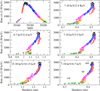 |
Fig. 1. Outburst light curve and HIDs for various hardness ratios, shown in the top-left corner of each diagram. Different colors represent different instances of the outburst as shown in the light curve (top-left panel): brown and red circles correspond to the rise of the outburst, black points to the peak, and blue, magenta, orange, and green circles to the decay of the outburst. |
First, three distinct branches can be seen in the HID. At a low count rate, the source moves horizontally in the HID, that is, significant spectral changes are seen for a very low change in count rate (green circles). At a certain intensity, the source turns upward and moves diagonally. As the intensity increases, the spectrum becomes harder. This branch contains most of the observations during the rise and decay of the outburst (brown, red, blue, magenta, and orange circles). The positive intensity-hardness ratio correlation stops near the peak of the outburst, when the source stabilizes, or even moves vertically (black circles).
Second, the soft part of the spectrum, E ≲ 5 keV, follows different tracks during the rise and decay of the outbursts. During the rise, the spectrum is harder than during the decay (compare the red and blue points in Fig. 1). This hysteresis effect decreases as the energy of the bands considered increases.
Third, we observed a break in hardness during the decay. At ∼700 cm s−1 (Lx ≈ 1.7 × 1037 erg s−1 in the 2–30 keV energy range), the source jumps from the decaying track to the rising track (note the discontinuity between the magenta and the orange circles in Fig. 1). Again, this effect is observed only at low energy.
3.3. Broadband noise
The fast temporal variability of the source is characterized by periodic (pulsations) and aperiodic (red noise) components. To investigate the broadband noise components associated with the aperiodic variability, we obtained the power spectral density (PSD) or simply the power spectrum by Fourier transform of the light curves in the 30–100 keV band. We used the HE instrument because it offers the largest effective area of the three instruments. To decrease the error in each frequency bin, the light curves were divided into segments and a fast Fourier transform was computed for each segment (see, e.g., van der Klis 1989, 2006). The final power spectrum is the average of the power spectra obtained for each segment.
The frequency interval covered by the power spectrum is given by [1/T, νnyq], where T is the duration of the segment and νnyq = 1/(2δt) is the Nyquist frequency; δt is the time resolution of the light curve. Because the variability of accreting X-ray pulsars at high frequencies is strongly suppressed (Reig & Nespoli 2013), most likely due to the viscous diffusion associated with accretion rate fluctuations (Mushtukov et al. 2019), the time resolution need not be too small. We set the highest frequency at 16 Hz (δt = 0.03125 s). The length of each interval was chosen to be 256 s, and hence the minimum frequency is ∼0.004 Hz. Since our goal is to study the correlated spectral-timing behavior of the source as a function of luminosity, we obtained PSDs at different instances of the outburst. At least two PSDs were obtained for each color interval, except for the observations with the lowest intensity (green circles); as such, given the low S/N, we generated one average PSD.
To study the broadband noise, we removed the contribution of the pulse flux from the light curves prior to the determination of the PSD (Finger et al. 1996; Revnivtsev et al. 2009). For each 1024-second segment (∼10 spin cycles), we obtained an average pulse profile. We replicated this profile and created a light curve with the same duration and binning as the original light curve. Then we subtracted the replicated light curve from the original one. The removal of the pulse peak and its harmonics were not always satisfactory, leaving some residuals. Since we used average light curves in the 30–100 keV range, the variability of the pulse profiles with energy (Mandal & Pal 2022) may contribute to those residuals.
We tried a second method that consisted in simply removing the frequency bins in the PSDs most affected by the pulsation and its harmonics. The results in terms of the value of the best-fit parameters and their dependence with luminosity were consistent with the pulse removal methodology.
To fit the PSDs, we followed two approaches. The first approach is that generally used in black-hole binaries. In these sources, it is common practice to describe the timing features with a function consisting of multiple Lorentzians, Li, where i defines the number of the component (Belloni et al. 2002). In 1A 0535+262, the Insight-HXMT PSD continuum in the 0.004–16 Hz frequency range is well described by three zero-centered Lorentzians, while another narrow Lorentzian is needed to fit the QPO. The characteristic frequency of Li is denoted νLi. This is the frequency where the component contributes most of its variance per logarithmic frequency interval and is defined as 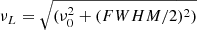 , where ν0 is the centroid frequency and FWHM is the Lorentzian full-width at half maximum. For a zero-centered Lorentzian, the characteristic frequency is simply half of its width.
The second approach is to use a broken-power-law model. Because many accreting pulsars display breaks in their power spectra (Revnivtsev et al. 2009; Mushtukov et al. 2019), the broken or double-broken power-law model has been used successfully in broadband noise analysis (Doroshenko et al. 2014, 2020). The model parameters of a broken power law are, in addition to the normalization, the break frequency, νbreak, and two power-law indices, Γ1 and Γ2. A Lorentzian is added to account for the QPO.
The broken power law fitted the PSD of 1A 0535+262 well at low luminosity (count rate below ∼275 count s−1 in 2–30 keV or 2 × 10⁻⁸ erg cm−2 s−1 in 1–100 keV). Above that value, the overall rms increases and an extra component is required. We tried fitting a double-broken power-law model, which included a second break frequency and a third power-law index. The fit improved considerably with the reduced χ2, typically changing from 2–4 to 1–2 for 65 and 62 degrees of freedom. The physical meaning of the higher frequency break is not clear. It has also been observed in the super-luminous X-ray pulsar Swift J0243.6+6124, albeit at luminosities above the Eddington limit (Doroshenko et al. 2020). Its frequency (∼5 − 7 Hz) is somewhat higher than the frequency observed in 1A 0535+262 (1–3 Hz). However, this can be understood by the natural shift of all the frequencies that characterize the aperiodic variability of pulsars with flux and by the different magnetic field strength. Figure 2 shows a representative PSD and the components of the two models considered. The Poisson noise was accounted for with a power law with index fixed to zero. The two models give comparable results in terms of the quality of the fit (reduced χ2), although the fitting parameters returned by the multi-Lorentzian model presented slightly less dispersion, especially at low luminosity. The reason may be the number of parameters involved in the fit (nine in the multi-Lorentzian model and six in the double-broken power-law model, excluding the QPO).
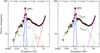 |
Fig. 2. Representative example of a power spectrum and model components used to fit the broadband noise: multi-Lorentzian model (left) and broken-power-law model (right). The Poisson noise was fitted with a power law with index fixed to zero (magenta line). The data correspond to observations taken during the period 22–25 November 2020. |
Figure 3 shows the dependence of the characteristic frequencies with 1–100 keV flux. The left panel displays the characteristic frequencies of the multi-Lorentzian fit, while the upper-right panel shows the break frequencies of the (double) broken-power-law model and the QPO. In all cases, as the X-ray luminosity increases, the characteristic frequencies shift to higher values. The second and third power-law indices of the double-broken power-law model did not change significantly during the outburst. To reduce the scatter in the frequency relation, we fixed them to their average values, Γ2 = 1.37 ± 0.05 and Γ3 = 1.66 ± 0.07. In contrast, the first power-law index, covering the lower frequency range, did show a smooth decline with luminosity (lower-right panel in Fig. 3) and was left free during the fit. The QPO frequency exhibits a very tight correlation regardless of the model used. As in previous studies (Revnivtsev et al. 2009; Doroshenko et al. 2014), we find that the QPO frequency is a factor of ∼3 − 4 lower than the break frequency. For a detailed study of the QPO variability during the 2020 outburst, we refer the reader to Ma et al. (in prep.).
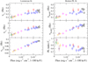 |
Fig. 3. Best-fit frequencies using the multi-Lorentzian model (left) and the broken-power-law model (right) as a function of X-ray flux. The color code is the same as in Fig. 1. |
4. Discussion
In this work we have investigated the changes in the spectral and timing continuum as a function of luminosity during the 2020 giant X-ray outburst of 1A 0535+262. Before discussing our results, we summarize here the different modes of accretion in accreting pulsars.
The strong magnetic field of the neutron star in accreting X-ray pulsars disrupts the accretion flow at some distance from the neutron star surface and forces the accreted matter to funnel down onto the polar caps, creating hot spots and an accretion column. The conditions prevailing in the accretion column define two accretion regimes: super- and sub-critical. These two regimes differ in the way the radiation pressure of the emitting plasma is capable of decelerating the accretion flow. At high luminosities in the super-critical regime, the radiation pressure dominates and the braking of the accreting matter flow is due to interaction with photons. A radiation-dominated shock stops the flow at a certain distance from the neutron star surface (Davidson & Ostriker 1973; Basko & Sunyaev 1976; Lyubarskii & Syunyaev 1982). In the sub-critical regime, the pressure of the radiation-dominated shock is not sufficient to stop the flow; it continues to the neutron star surface, where it is decelerated by multiple Coulomb scattering with thermal electrons and nuclear collisions with atmospheric protons (Burnard et al. 1991; Harding 1994). A key parameter is the luminosity at which the source transits from the sub- to the super-critical regime. This is known as the critical luminosity, Lcrit (Basko & Sunyaev 1976; Becker et al. 2012; Mushtukov et al. 2015).
At even lower luminosity, the Coulomb atmosphere dissipates and the matter goes all the way to the neutron star surface, possibly passing through a gas-mediated shock (Langer & Rappaport 1982). The luminosity at which this transition occurs is usually referred to as Lcoul (see Eq. (54) in Becker et al. 2012). Collisions may also result in the excitation of electrons to upper Landau levels, whose subsequently de-excitation generates cyclotron photons (Mushtukov et al. 2021). The energy spectrum at low accretion rates is characterized by two broad components that peak at ∼5 − 7 keV and ∼30 − 50 keV (Tsygankov et al. 2019). In the model by Mushtukov et al. (2021), the low energy hump corresponds to Comptonized thermal radiation and the high energy hump to Comptonized cyclotron photons.
Recent developments in the field have shown that this general picture should be modified at the highest luminosity. In super-Eddington X-ray pulsars (so far, only Swift J0243.6+6124), a third regime has been suggested, which would be associated with the transition of the inner regions of the accretion disk from the standard gas-pressure-dominated state to the radiation-pressure-dominated state. This transition would occur at a luminosity one order of magnitude higher than the transition from the sub-critical to the super-critical regime (Doroshenko et al. 2020).
4.1. Hardness-intensity diagram and accretion regimes
A model-independent way to study the X-ray spectral continuum is through changes in the count rate in two different energy bands (hardness ratio). The HID has proven to be a useful tool for studying spectral states not only in black-hole binaries and low-mass X-ray binaries (see e.g. van der Klis 2006; Belloni 2010) but also in high-mass X-ray binaries (Reig 2008; Reig & Nespoli 2013).
Reig & Nespoli (2013) investigated the X-ray color changes during type II outbursts of nine BeXBs. They defined two main branches that they called horizontal and diagonal and attributed to the sub- and super-critical accretion states. Not all sources displayed the two branches. In fact, only four of the nine studied sources transited to a super-critical state. Reig & Nespoli (2013) concluded that in order to see a transition to the super-critical state and hence observe a clear diagonal branch in the HID, the outburst peak source luminosity must be several times the critical luminosity.
Although the two branches can be clearly distinguished and identified by the direction of motion of the source in the HID – in the horizontal branch the source becomes harder as the intensity increases, whereas in the diagonal branch the source softens as it brightens – this terminology is somewhat confusing as the horizontal branch normally appears inclined when a logarithmic scale is used (e.g., compare Figs. 2 and 3 in Reig & Nespoli 2013).
In this work we refer to the branches by their dependence with intensity. Therefore, the almost horizontal branch at the lowest count rate (green filled circles in Fig. 1), which is formed by the first and last recorded observations of the outburst, is the low-intensity branch (LIB). The inclined branch populated by all the observations of the rise and decay at intermediate count rates is intermediate-intensity branch (IIB). Finally, the black circles that correspond to the peak of the outburst define the high-intensity branch (HIB). The horizontal and diagonal branches in the terminology of Reig & Nespoli (2013) would be the IIB and HIB, respectively. In the case of 1A 0535+262, only the beginning of the HIB would be visible. The LIB (green circles) is reported here for the first time.
Which and how many branches appear in the HID clearly depends on the sensitivity of the detectors, on the range in count rate covered by the observations, and on the value of the critical luminosity. The critical luminosity is different for different sources as it strongly depends on the geometry of the accretion column and the magnetic field (Basko & Sunyaev 1976; Becker et al. 2012; Mushtukov et al. 2015). The larger the magnetic field, the higher the critical luminosity and the longer the source spends in the sub-critical regime (IIB). Thus, the reason that 1A 0535+262 does not show a well-developed super-critical branch (HIB) is the high value of the critical luminosity in this system, Lcrit ∼ 6.7 × 1037 erg s−1 (Kong et al. 2021). The maximum luminosity measured during the outburst is not significantly larger than this value. Because the ratio Lpeak/Lcrit is not much larger than 1, the HIB (i.e. super-critical) branch does not extend toward the left and only the initial instances of this branch are observed in 1A 0535+262. Had the source luminosity increased further, we would have presumably seen the HIB extending left toward a lower hardness ratio as in 4U 0115+63, EXO 2030+375, KS 1947+300, and V 0332+53 (Reig & Nespoli 2013). A transition to the super-critical regime is supported by a detailed analysis of the energy spectra, which shows sudden changes in the correlation of the photon index of the power-law component (Mandal & Pal 2022) and the cyclotron line (Kong et al. 2021) with luminosity.
The LIB (green circles in Fig. 1) is not present in any of the sources studied by Reig & Nespoli (2013) (perhaps with the exception of XTE J0658-073). Following the interpretation that the IIB and HIB correspond to the sub-critical and super-critical accretion regimes, the LIB could be associated with the transition from the Coulomb stopping to gas shock, that is, when both the radiative shock and the Coulomb atmosphere have disappeared or are too weak. The average luminosity during the LIB is Lx ≈ 6 × 1036 erg s−1, which approximately agrees with Lcoul (Becker et al. 2012) for typical parameters of neutron stars and assuming a magnetic field of ∼4 × 10¹² G. At this and lower luminosity, the accretion flow is decelerated by collisions between particles. The LIB is characterized by a very fast softening of the spectrum as the count rate decreases. As the accretion rate decreases, we would expect the collisions of the accreting particles with the electrons of the neutron star atmosphere to become less efficient. Indeed, in the framework of the Mushtukov et al. (2021) model, the relative contribution of the thermal component with respect to the cyclotron Comptonized component increases as the luminosity decreases (Tsygankov et al. 2019).
Another interesting finding is the sudden jump from the decaying track to the rising track at around 700 c/s (2–30 keV), or 2 × 1037 erg s−1, in the low energy hardness ratios (4–7/2–4 and 7–10/2–4) in Fig. 1 (transition from the magenta to the orange circles). The effect is less important at higher energies. The amplitude of change in the hardness ratio is 0.05 for HR = 4–7/2–4, 0.02 for HR = 7–10/3–5, 0.01 for HR = 7–10/4–7, and non-existent for HR = 15–30/10–15. It is not clear what could lead to this effect. One may argue that the count rate is not a good proxy for the accretion rate. However, the discontinuity remains even when we use luminosity or flux instead of intensity.
4.2. Broadband noise variability
The accretion process generates strong aperiodic variability that manifests as broadband noise in the power spectrum of BeXBs (Reig 2008; Revnivtsev et al. 2009; Tsygankov et al. 2012; Reig & Nespoli 2013; Doroshenko et al. 2014, 2020; Mushtukov et al. 2019). The PSDs display a characteristic break that has been associated with the truncation radius of the accretion disk, at the location where the accretion disk meets the magnetosphere (Revnivtsev et al. 2009), or with the timescale of the dynamo process, which is assumed to be responsible for the initial fluctuations in viscosity (Mushtukov et al. 2019) that propagate through the disk and give rise to the aperiodic variability (Lyubarskii 1997; Churazov et al. 2001).
Quasi-periodic oscillations are another prominent feature in the power spectrum of 1A 0535+262 (Finger et al. 1996; Camero-Arranz et al. 2012, see also Ma et al. (in prep.). Most models locate the origin of the QPO in the interplay between the accretion disk and the magnetosphere. The break frequency would be associated with the timescales on which accretion rate fluctuations occur within the disk, while QPOs would be associated with the Keplerian timescales at the inner edge of the accretion disk and the magnetosphere boundary. The break frequency originating in a truncated disc is expected to correlate with the Keplerian frequency at the magnetosphere.
A general property of the break and QPO frequencies is that they shift to higher values as the X-ray luminosity increases. This result is naturally explained by the relationship between mass accretion rate and the size of the magnetosphere. The magnetospheric radius scales with the mass accretion rate as Rm ∝ Ṁ−2/7; as Ṁ increases, the luminosity increases and the magnetosphere shrinks. The accretion disk radius decreases, and the characteristic frequency at the inner edge of the disk increases. Figure 3 shows the evolution of the characteristic frequencies of the broadband noise as a function of flux.
The large peak luminosity displayed by 1A 0535+262 during the 2020 outburst allows us to study the frequency-luminosity correlation on a broader range in X-ray luminosity, as shown in Fig. 4. This correlation initially covered two orders of magnitude in flux (Revnivtsev et al. 2009). Doroshenko et al. (2014) extended it at the lower end by analyzing observations close to quiescence. Here we extend the correlation at the higher end up to 10−7 erg cm−2 s−1. Thus, the correlation now holds for more than four orders of magnitude in X-ray flux.
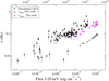 |
Fig. 4. Break frequencies as a function of X-ray flux. Data are from XMM-Newton, RXTE/PCA (from Doroshenko et al. 2014), and Insight- HXMT/HE. |
Although there is large scatter in the plot, we notice a flattening of the correlation at the highest flux, which is also apparent in Fig. 3. In the framework of the perturbation propagation model, the break frequency observed in the PSD is related to the variability generated at the inner edge of the disk (Revnivtsev et al. 2009). Therefore, it might be that the inner parts of the accretion disk reached the closest possible distance to the neutron star at the highest luminosities.
4.3. Hysteresis
Hysteresis patterns are commonly observed in black-hole binaries (Miyamoto et al. 1995; Begelman & Armitage 2014; Weng et al. 2021) and low-mass X-ray binaries (Muñoz-Darias et al. 2014). In this context, hysteresis means that certain spectral and timing parameters have different values depending on whether the source is in the rising phase of the outburst or in the declining phase despite the luminosity being similar. Although the number of accreting pulsars investigated is not large, some cases of hysteretic behavior have been reported. Hysteresis is not only seen in the HID (Reig 2008) but also in the pulse fraction (Wang et al. 2020) and the spin rate (Filippova et al. 2017).
In 1A 0535+262 the hysteresis pattern appears both in the spectral continuum and the broadband noise. The color analysis reveals that for the same intensity the spectral hardness is higher during the rise than during the decay of the outburst (compare the red and blue circles in Fig. 1). Also, the hysteresis pattern is most prominent at low energies. The pattern disappears as we consider higher energy bands (E ≳ 4 keV). The softer part of the spectrum of accreting pulsars is associated with thermal emission from the polar caps and/or the base of the accretion column. In fact, Kong et al. (2021) found that two blackbody components were needed to fit the spectrum of 1A 0535+262 during the 2020 outburst. Interestingly, both the temperature and size of the emitting region of the two thermal components exhibited hysteresis, with the temperatures being higher and the emitting region smaller during the rise (see Fig. 5 in Kong et al. 2021). The base of the accretion column and/or the polar cap area appear to be more compact during its formation (rise) than during its dissipation (decay). The different path during the rise and decay is also apparent in the photon index of the power-law component (Kong et al. 2021). Likewise, the characteristic frequency of the main broadband component (νLor2 and νbreak1) was higher during the rise (red circles in Fig. 3). The higher frequencies may simply mean that the inner part of the accretion disk moved closer to the neutron star during the rise compared to the same luminosity during the decay.
The fact that the hysteresis is seen in both spectral and timing parameters sets tight constraints on the models that seek to explain this behavior. Spectral variability occurs very close to the neutron star surface in the accretion column, while aperiodic variability originates in the accretion disk. The structure that links these two emission sites is the magnetosphere. Therefore, although there is no general consensus on the origin of the hysteresis effect in accreting pulsars, it appears to be related to a different size of the magnetosphere during the rise and decay, which would also translate into changes in the configuration of the accretion column. A smaller magnetospheric radius was also invoked to explained the higher spin-up rate in the BeXB V 0332+53 during the rise of its 2015 giant outburst (Doroshenko et al. 2017).
What causes this different size is unclear. It might be due to a variable magnetic field strength (Cusumano et al. 2016) or a change in the emission region geometry (Poutanen et al. 2013; Doroshenko et al. 2017, but see Kylafis et al. 2021). The fact that the energy of the cyclotron line was systematically lower during the rise (Kong et al. 2021) might indicate a weaker magnetic field. However, it is not clear how the magnetic field strength can change on such timescales. In V 0332+53, the evolution of the energy of the cyclotron line was opposite to that of 1A 0535+262, with a drop in the cyclotron line energy during the declining part. Therefore, it is difficult to think of a mechanism that would change the magnetic field strength in opposite ways for two apparently similar sources. Equally, it is not clear what could lead to a different evolution of the inner disk radius in the two sources that would favor a smaller magnetosphere during the rise in one case and a larger magnetosphere in the other, also during the rising phase. As pointed out by Kong et al. (2021), perhaps the different spin period of the two sources – V 0332+53 is a fast pulsar (Pspin = 4.4 s), while 1A 0535+262 is a slow pulsar (Pspin = 103 s) – leads to a different interplay between the accretion column and the magnetosphere. We also note that the optical counterpart to V 0332+53 is more massive (O8–9V star) and orbits at a significantly closer distance (Porb = 34 days) than that of 1A 0535+262 (B0III star, Porb = 111 days).
5. Conclusion
The November 2020 bright X-ray outburst of 1A 0535+262 allowed us to study the spectral-timing properties of this accreting pulsar at very high luminosity. Despite the different origin of the spectral variability (accretion column) and the broadband noise (accretion disk), both kinds of variability provide evidence for a different behavior depending on whether the source was on the rise or on the decay of the outburst. The hysteresis pattern is dominant at intermediate luminosity and low energy and appears to be related to a variable magnetospheric radius. At similar luminosity, the inner parts of the accretion disk would move closer to the neutron star during the rise. The HID appears to be a useful tool for identifying accretion regimes. We observe three different branches that we identified with accretion at LX ≳ Lcrit (HIB) and two branches associated with the sub-critical regime, when Lcoul < LX < Lcrit (IIB) and when LX ∼ Lcoul (LIB). Because of its high magnetic field, the critical luminosity in 1A 0535+262 is high and the source only traces the beginning of the HIB. We have extended the correlation between the break frequency of the broadband noise and the luminosity above LX > 2 × 1037 erg s−1, and now it holds over four orders of magnitude in luminosity.
Acknowledgments
ZS and TL acknowledge the supports of the National Key R&D Program of China (2021YFA0718500) and the National Natural Science Foundation of China under grant U1838201, U1838202, and 11733009. L.T. acknowledges funding support from the National Natural Science Foundation of China (NSFC) under grant No. 12122306 and the CAS Pioneer Hundred Talent Program Y8291130K2. This work has made use of the data from the Insight-HXMT mission, a project funded by China National Space Administration (CNSA) and the Chinese Academy of Sciences (CAS).
References
- Acciari, V. A., Aliu, E., Araya, M., et al. 2011, ApJ, 733, 96 [NASA ADS] [CrossRef] [Google Scholar]
- Bailer-Jones, C. A. L., Rybizki, J., Fouesneau, M., Demleitner, M., & Andrae, R. 2021, AJ, 161, 147 [Google Scholar]
- Basko, M. M., & Sunyaev, R. A. 1976, MNRAS, 175, 395 [Google Scholar]
- Becker, P. A., Klochkov, D., Schönherr, G., et al. 2012, A&A, 544, A123 [NASA ADS] [CrossRef] [EDP Sciences] [Google Scholar]
- Begelman, M. C., & Armitage, P. J. 2014, ApJ, 782, L18 [NASA ADS] [CrossRef] [Google Scholar]
- Belloni, T. M. 2010, States and Transitions in Black Hole Binaries, ed. T. Belloni, 794, 53 [Google Scholar]
- Belloni, T., Psaltis, D., & van der Klis, M. 2002, ApJ, 572, 392 [NASA ADS] [CrossRef] [Google Scholar]
- Burnard, D. J., Arons, J., & Klein, R. I. 1991, ApJ, 367, 575 [CrossRef] [Google Scholar]
- Camero-Arranz, A., Finger, M. H., Wilson-Hodge, C. A., et al. 2012, ApJ, 754, 20 [NASA ADS] [CrossRef] [Google Scholar]
- Cao, X., Jiang, W., Meng, B., et al. 2020, Sci. China Phys. Mech. Astron., 63 [Google Scholar]
- Chen, Y., Cui, W., Li, W., et al. 2020, Sci. China Phys. Mech. Astron., 63 [Google Scholar]
- Churazov, E., Gilfanov, M., & Revnivtsev, M. 2001, MNRAS, 321, 759 [NASA ADS] [CrossRef] [Google Scholar]
- Clark, J. S., Steele, I. A., Coe, M. J., & Roche, P. 1998a, MNRAS, 297, 657 [NASA ADS] [CrossRef] [Google Scholar]
- Clark, J. S., Tarasov, A. E., Steele, I. A., et al. 1998b, MNRAS, 294, 165 [CrossRef] [Google Scholar]
- Clark, J. S., Lyuty, V. M., Zaitseva, G. V., et al. 1999, MNRAS, 302, 167 [NASA ADS] [CrossRef] [Google Scholar]
- Coe, M. J., Carpenter, G. F., Engel, A. R., & Quenby, J. J. 1975, Nature, 256, 630 [NASA ADS] [CrossRef] [Google Scholar]
- Cusumano, G., La Parola, V., D’Aì, A., et al. 2016, MNRAS, 460, L99 [NASA ADS] [CrossRef] [Google Scholar]
- Davidson, K., & Ostriker, J. P. 1973, ApJ, 179, 585 [NASA ADS] [CrossRef] [Google Scholar]
- De Loore, C., Giovannelli, F., van Dessel, E. L., et al. 1984, A&A, 141, 279 [NASA ADS] [Google Scholar]
- Doroshenko, V., Santangelo, A., Doroshenko, R., et al. 2014, A&A, 561, A96 [NASA ADS] [CrossRef] [EDP Sciences] [Google Scholar]
- Doroshenko, V., Tsygankov, S. S., Mushtukov, A. E. A., et al. 2017, MNRAS, 466, 2143 [NASA ADS] [CrossRef] [Google Scholar]
- Doroshenko, V., Zhang, S. N., Santangelo, A., et al. 2020, MNRAS, 491, 1857 [Google Scholar]
- Filippova, E. V., Mereminskiy, I. A., Lutovinov, A. A., Molkov, S. V., & Tsygankov, S. S. 2017, Astron. Lett., 43, 706 [NASA ADS] [Google Scholar]
- Finger, M. H., Wilson, R. B., & Chakrabarty, D. 1996, A&AS, 120, 209 [NASA ADS] [Google Scholar]
- Gnedin, I. N., Khozov, G. V., & Larionov, V. M. 1983, Ap&SS, 93, 207 [NASA ADS] [CrossRef] [Google Scholar]
- Haigh, N. J., Coe, M. J., Steele, I. A., & Fabregat, J. 1999, MNRAS, 310, L21 [NASA ADS] [CrossRef] [Google Scholar]
- Haigh, N. J., Coe, M. J., & Fabregat, J. 2004, MNRAS, 350, 1457 [NASA ADS] [CrossRef] [Google Scholar]
- Hao, J. X., Huang, L., & Guo, Z. H. 1996, A&A, 308, 499 [NASA ADS] [Google Scholar]
- Harding, A. K. 1994, in The Evolution of X-ray Binariese, eds. S. Holt, & C. S. Day, Am. Inst. Phys. Conf. Ser., 308, 429 [CrossRef] [Google Scholar]
- Hudec, R. 1975, Zentralinstitut fuer Astrophysik Sternwarte Sonneberg Mitteilungen ueber Veraenderliche Sterne, 7, 29 [Google Scholar]
- James, M., Paul, B., Devasia, J., & Indulekha, K. 2010, MNRAS, 407, 285 [NASA ADS] [CrossRef] [Google Scholar]
- Janot-Pacheco, E., Motch, C., & Mouchet, M. 1987, A&A, 177, 91 [NASA ADS] [Google Scholar]
- Kong, L. D., Zhang, S., Ji, L., et al. 2021, ApJ, 917, L38 [NASA ADS] [CrossRef] [Google Scholar]
- Kylafis, N. D., Trümper, J. E., & Loudas, N. A. 2021, A&A, 655, A39 [NASA ADS] [CrossRef] [EDP Sciences] [Google Scholar]
- Langer, S. H., & Rappaport, S. 1982, ApJ, 257, 733 [NASA ADS] [CrossRef] [Google Scholar]
- Liu, C., Zhang, Y., Li, X., et al. 2020, Sci. China Phys. Mech. Astron., 63 [Google Scholar]
- Lyubarskii, Y. E. 1997, MNRAS, 292, 679 [Google Scholar]
- Lyubarskii, Y. E., & Syunyaev, R. A. 1982, Sov. Astron. Lett., 8, 330 [Google Scholar]
- Lyuty, V. M., & Zaĭtseva, G. V. 2000, Astron. Lett., 26, 9 [NASA ADS] [CrossRef] [Google Scholar]
- Mandal, M., & Pal, S. 2022, MNRAS, 511, 1121 [NASA ADS] [CrossRef] [Google Scholar]
- Migliari, S., Tudose, V., Miller-Jones, J. C. A., et al. 2011, Astron. Tel., 3198, 1 [Google Scholar]
- Miyamoto, S., Kitamoto, S., Hayashida, K., & Egoshi, W. 1995, ApJ, 442, L13 [NASA ADS] [CrossRef] [Google Scholar]
- Moritani, Y., Nogami, D., Okazaki, A. T., et al. 2013, PASJ, 65, 83 [NASA ADS] [Google Scholar]
- Motch, C., Belloni, T., Buckley, D., et al. 1991, A&A, 246, L24 [NASA ADS] [Google Scholar]
- Muñoz-Darias, T., Fender, R. P., Motta, S. E., & Belloni, T. M. 2014, MNRAS, 443, 3270 [CrossRef] [Google Scholar]
- Murdin, P. 1975, IAU Circ., 2784, 1 [NASA ADS] [Google Scholar]
- Mushtukov, A. A., Suleimanov, V. F., Tsygankov, S. S., & Poutanen, J. 2015, MNRAS, 447, 1847 [NASA ADS] [CrossRef] [Google Scholar]
- Mushtukov, A. A., Lipunova, G. V., Ingram, A., et al. 2019, MNRAS, 486, 4061 [NASA ADS] [CrossRef] [Google Scholar]
- Mushtukov, A. A., Suleimanov, V. F., Tsygankov, S. S., & Portegies Zwart, S. 2021, MNRAS, 503, 5193 [Google Scholar]
- Naik, S., Mathew, B., Banerjee, D. P. K., Ashok, N. M., & Jaiswal, R. R. 2012, Res. Astron. Astrophys., 12, 177 [CrossRef] [Google Scholar]
- Payne, B. J., & Coe, M. J. 1987, MNRAS, 225, 985 [NASA ADS] [CrossRef] [Google Scholar]
- Persi, P., Ferrari-Toniolo, M., Spada, G., et al. 1979, MNRAS, 187, 293 [NASA ADS] [Google Scholar]
- Poutanen, J., Mushtukov, A. A., Suleimanov, V. F., et al. 2013, ApJ, 777, 115 [NASA ADS] [CrossRef] [Google Scholar]
- Rappaport, S., Joss, P. C., Bradt, H., Clark, G. W., & Jernigan, J. G. 1976, ApJ, 208, L119 [NASA ADS] [CrossRef] [Google Scholar]
- Reig, P. 2008, A&A, 489, 725 [NASA ADS] [CrossRef] [EDP Sciences] [Google Scholar]
- Reig, P., & Nespoli, E. 2013, A&A, 551, A1 [NASA ADS] [CrossRef] [EDP Sciences] [Google Scholar]
- Revnivtsev, M., Churazov, E., Postnov, K., & Tsygankov, S. 2009, A&A, 507, 1211 [CrossRef] [EDP Sciences] [Google Scholar]
- Rosenberg, F. D., Eyles, C. J., Skinner, G. K., & Willmore, A. P. 1975, Nature, 256, 628 [NASA ADS] [CrossRef] [Google Scholar]
- Taranova, O. G., & Shenavrin, V. I. 2017, Astron. Rep., 61, 983 [NASA ADS] [CrossRef] [Google Scholar]
- Tsygankov, S. S., Krivonos, R. A., & Lutovinov, A. A. 2012, MNRAS, 421, 2407 [CrossRef] [Google Scholar]
- Tsygankov, S. S., Doroshenko, V., Mushtukov, A. E. A., et al. 2019, MNRAS, 487, L30 [NASA ADS] [CrossRef] [Google Scholar]
- Tudose, V., Migliari, S., Miller-Jones, J. C. A., et al. 2010, Astron. Tel., 2798, 1 [NASA ADS] [Google Scholar]
- van der Klis, M. 1989, in NATO Advanced Science Institutes (ASI) Series C, eds. H. Ögelman, & E. P. J. van den Heuvel, 262, 27 [Google Scholar]
- van der Klis, M. 2006, Rapid X-ray Variability, eds. W. H. G. Lewin, & M. van der Klis, 39 [Google Scholar]
- Wang, P. J., Kong, L. D., Zhang, S., et al. 2020, MNRAS, 497, 5498 [NASA ADS] [CrossRef] [Google Scholar]
- Weng, S.-S., Cai, Z.-Y., Zhang, S.-N., et al. 2021, ApJ, 915, L15 [NASA ADS] [CrossRef] [Google Scholar]
- Wu, C. C., Panek, R. J., Holm, A. V., Schmitz, M., & Swank, J. H. 1983, PASP, 95, 391 [CrossRef] [Google Scholar]
- Yan, J., Li, H., & Liu, Q. 2012, ApJ, 744, 37 [NASA ADS] [CrossRef] [Google Scholar]
- Zaitseva, G. V. 2005, Astron. Lett., 31, 103 [NASA ADS] [CrossRef] [Google Scholar]
- Zhang, S.-N., Li, T., Lu, F., et al. 2020, Sci. China Phys. Mech. Astron., 63 [Google Scholar]
All Tables
All Figures
|
Fig. 1. Outburst light curve and HIDs for various hardness ratios, shown in the top-left corner of each diagram. Different colors represent different instances of the outburst as shown in the light curve (top-left panel): brown and red circles correspond to the rise of the outburst, black points to the peak, and blue, magenta, orange, and green circles to the decay of the outburst. |
| In the text | |
|
Fig. 2. Representative example of a power spectrum and model components used to fit the broadband noise: multi-Lorentzian model (left) and broken-power-law model (right). The Poisson noise was fitted with a power law with index fixed to zero (magenta line). The data correspond to observations taken during the period 22–25 November 2020. |
| In the text | |
|
Fig. 3. Best-fit frequencies using the multi-Lorentzian model (left) and the broken-power-law model (right) as a function of X-ray flux. The color code is the same as in Fig. 1. |
| In the text | |
|
Fig. 4. Break frequencies as a function of X-ray flux. Data are from XMM-Newton, RXTE/PCA (from Doroshenko et al. 2014), and Insight- HXMT/HE. |
| In the text | |
Current usage metrics show cumulative count of Article Views (full-text article views including HTML views, PDF and ePub downloads, according to the available data) and Abstracts Views on Vision4Press platform.
Data correspond to usage on the plateform after 2015. The current usage metrics is available 48-96 hours after online publication and is updated daily on week days.
Initial download of the metrics may take a while.