| Issue |
A&A
Volume 659, March 2022
|
|
|---|---|---|
| Article Number | A27 | |
| Number of page(s) | 15 | |
| Section | Stellar structure and evolution | |
| DOI | https://doi.org/10.1051/0004-6361/202142194 | |
| Published online | 02 March 2022 | |
Models of pulsationally assisted gravitationally confined detonations with different ignition conditions
1
Heidelberger Institut für Theoretische Studien, Schloss-Wolfsbrunnenweg 35, 69118 Heidelberg, Germany
e-mail: This email address is being protected from spambots. You need JavaScript enabled to view it.
2
Zentrum für Astronomie der Universität Heidelberg, Institut für Theoretische Astrophysik, Philosophenweg 12, 69120 Heidelberg, Germany
3
School of Mathematics and Physics, Queen’s University Belfast, Belfast BT7 1NN, UK
Received:
10
September
2021
Accepted:
15
November
2021
Abstract
Over the past decades, many explosion scenarios for Type Ia supernovae have been proposed and investigated including various combinations of deflagrations and detonations in white dwarfs of different masses up to the Chandrasekhar mass. One of these is the gravitationally confined detonation model. In this case a weak deflagration burns to the surface, wraps around the bound core, and collides at the antipode. A subsequent detonation is then initiated in the collision area. Since the parameter space for this scenario, that is, varying central densities and ignition geometries, has not been studied in detail, we used pure deflagration models of a previous parameter study dedicated to Type Iax supernovae as initial models to investigate the gravitationally confined detonation scenario. We aim to judge whether this channel can account for one of the many subgroups of Type Ia supernovae, or even normal events. To this end, we employed a comprehensive pipeline for three-dimensional Type Ia supernova modeling that consists of hydrodynamic explosion simulations, nuclear network calculations, and radiative transfer. The observables extracted from the radiative transfer are then compared to observed light curves and spectra. The study produces a wide range in masses of synthesized 56Ni ranging from 0.257 to 1.057 M⊙, and, thus, can potentially account for subluminous as well as overluminous Type Ia supernovae in terms of brightness. However, a rough agreement with observed light curves and spectra can only be found for 91T-like objects. Although several discrepancies remain, we conclude that the gravitationally confined detonation model cannot be ruled out as a mechanism to produce 91T-like objects. However, the models do not provide a good explanation for either normal Type Ia supernovae or Type Iax supernovae.
Key words: hydrodynamics / nuclear reactions, nucleosynthesis, abundances / radiative transfer / methods: numerical / supernovae: general / supernovae: individual: SN 1991T
© ESO 2022
1. Introduction
Despite several decades of research, the questions of the progenitor systems of Type Ia supernovae (SNe Ia), and their explosion mechanism, remain open. A common basis for modeling different conceivable explosion scenarios is the origin of SNe Ia from the thermonuclear disruptions of carbon-oxygen (CO, Hoyle & Fowler 1960; Arnett 1969), oxygen-neon (ONe, Marquardt et al. 2015; Kashyap et al. 2018), hybrid carbon-oxygen-neon (CONe, Denissenkov et al. 2015; Kromer et al. 2015; Bravo et al. 2016), or helium-carbon-oxygen (Pakmor et al. 2021) white dwarf (WD) stars in a binary system. Whether the pre-explosion WD has reached the Chandrasekhar mass (MCh) or whether it remains significantly below this limit is not clear yet. In fact, it may well be possible that more than one progenitor and explosion mechanism is needed to account for the observed sample of SNe Ia given the variety of peculiar subclasses that have been identified (Taubenberger 2017; Jha 2017). The nature of the binary companion of the exploding WD is yet another open question since it is not clear whether it is a nondegenerate star, for example, a main sequence, red giant, or asymptotic giant branch star (Whelan & Iben 1973), or another WD (Iben & Tutukov 1984). Finally, the reason for the explosion and the combustion mechanism are unknown. The WD might explode due to an interaction with its binary companion via accretion or due to a merger with the latter, and the thermonuclear flame can propagate as a subsonic deflagration or a supersonic detonation front (e.g., Röpke 2016). These possibilities leave room for a plethora of explosion scenarios (see Hillebrandt et al. 2013, for a review) trying to explain the typical features of the bulk of so-called normal SNe Ia as well as the various subclasses. Here, we focus solely on explosions of MCh WDs.
Specifically, we extend the models of asymmetric deflagrations in MCh WDs of Lach et al. (2022, hereafter L21), and trigger detonations in late stages of the explosion. The models presented in that study were ignited asymmetrically in a single spot, and, hence, lead to weak deflagrations ejecting only little mass. The deflagration ashes rush across the still bound object and collide at the opposite side. Therefore, they can serve as a starting point for the investigation of the gravitationally confined detonation (GCD) scenario first investigated by Plewa et al. (2004). In this scenario, a detonation is initated in the collision region leading to a healthy explosion disrupting the whole star. The goal of our study is to investigate two main properties of these models. First, we explore whether this mechanism is capable of reproducing the brightness variation of normal SNe Ia or even extending to subluminous events. Second, the effects of the predicted composition inversion in comparison to 1D SN Ia (see e.g., Nomoto et al. 1984; Khokhlov et al. 1993) models of the canonical delayed detonation (DD) scenario (Gamezo et al. 2005; Röpke & Niemeyer 2007; Sim et al. 2013) on the predicted observables are examined. By construction, the deflagration products remain in the central parts of the ejecta in 1D models. In 3D DD simulations, the composition is not strictly stratified. Deflagration ashes extend out to high ejecta velocities while material composed of lighter elements sinks down toward the center because of the buoyancy instabilitiy during the initial deflagration phase. In the GCD model this effect is most strongly pronounced. A complete inversion of the ejecta composition compared to the 1D models is observed: the deflagration products enshroud the detonation ashes. While Kasen & Plewa (2007) conclude that the spectrum of SN 1994D can be matched by their GCD model, Baron et al. (2008) and Seitenzahl et al. (2016) find it difficult to bring the large abundances of iron group elements (IGEs) in the outer layers in agreement with observations (see discussion in Sect. 2).
Because of the restricted spatial resolution of the regions where the detonation potentially triggers, the mechanism for the initiation of the detonation wave cannot be followed consistently within this study. According to Seitenzahl et al. (2009a) a resolution of at least a few 100 meters per cell is required. We emphasize that the numerical methods used in this work are not appropriate to conclusively verify whether a detonation is ignited or not (see Sect. 4). Therefore, we only give plausibility arguments and follow a what-if-approach to explore the consequences of an assumed detonation initiation. Because of this uncertainty, the occurrence of a detonation is not necessarily a contradiction to the notion that Type Iax supernovae (SNe Iax) may arise from weak deflagrations in MCh WDs Branch et al. (2004), Phillips et al. (2007), Kromer et al. (2013), Long et al. (2014), Fink et al. (2014), L21. Although a detonation is possible in the collision region it is not guaranteed that it also occurs in every realization in nature. Furthermore, we note that the GCD mechanism relies on the absence of a spontaneous deflagration-to-detonation transition (DDT) before the deflagration breaks out of the surface. Also in this case, the question – whether DDTs occur in unconfined media remains an open issue and topic of active research (Oran & Gamezo 2007; Woosley et al. 2009; Poludnenko et al. 2011, but see Poludnenko et al. 2019 for a recently suggested mechanism).
The paper is structured in the following way: we first discuss the GCD explosion mechanism and its implications in detail in Sect. 2, and, then give a brief overview of the employed codes and our initial setup in Sect. 3. This is followed by a description of the detonation initiation mechanism and conditions relevant for this study in Sect. 4. Section 5 then covers the results of the hydrodynamic simulations and the postprocessing step. In Sect. 6 we present synthetic observables and compare them to observations. Finally, our conclusions can be found in Sect. 7.
2. Explosion model
As mentioned above, in a previous study (L21), we investigate explosions of MCh WDs that result from ignitions of a deflagration flame in a single spot off-center of the star as suggested by simmering phase simulations by Zingale et al. (2009, 2011) and Nonaka et al. (2012). Such models had been proposed to explain the class of SNe Iax and we confirm that a large part of the luminosity range observed for these objects can be reproduced in the context of the assumed explosion scenario. The overall agreement of those models with observational data of SNe Iax (light curves and spectra) is reasonable, but not perfect. In particular, the observables of the lowest-luminosity members of the SN Iax class are not satisfactorily reproduced by our models. In the scenario of a subsonic deflagration ignited in a single (or a few) spark(s) off-center in a MCh WD star, the energy released by the nuclear burning does not completely unbind the object and a bound remnant is left behind. But even multispot ignition scenarios – also capable of unbinding the entire WD star – produce 56Ni masses and explosion energies reaching the faint end of normal SNe Ia at best (Fink et al. 2014). A DD in such models can produce brighter events and approximately cover the range of observed normal SNe Ia (Gamezo et al. 2005; Maeda et al. 2010a; Röpke & Niemeyer 2007; Seitenzahl et al. 2013a). Observables predicted from these models are again in reasonable agreement with data, however, important trends and relations such as the width-luminosity relation employed to calibrate SNe Ia as cosmological distance indicators (Phillips 1993) are not fully reproduced by current multidimensional models (Kasen et al. 2009; Sim et al. 2013). We note, however, that it has been demonstrated that a full treatment of nonlocal thermodynamic equilibrium (NLTE) effects is important for detailed modeling, including at phases relevant to studying the width-luminosity relation (e.g., Blondin et al. 2013; Dessart et al. 2014; Shen et al. 2021). Since multidimensional studies currently lack full NLTE treatments further work is therefore still needed to fully quantify the extent to which such models can agree with observations. As mentioned above, the mechanism triggering the required spontaneous transition of the combustion wave from deflagration to detonation remains unclear.
For the single-spot off-center ignited MCh WD models considered by L21, triggering of a detonation in a late phase of the explosion process is also a possibility. Such scenarios have been discussed by Plewa et al. (2004) as gravitationally confined detonations and were later investigated in more detail by Plewa (2007), Townsley et al. (2007), Röpke et al. (2007), Jordan et al. (2008, 2009), Meakin et al. (2009), Seitenzahl et al. (2009b, 2016), García-Senz et al. (2016), and Byrohl et al. (2019). The idea is that the deflagration flame rises toward the surface of the WD and sweeps around the gravitationally bound core. Subsequently, the ashes collide on the opposite side and a detonation is ignited in the collision region. There, an inward and outward moving jet form and material is compressed and heated at the head of the inward moving jet until necessary conditions for a detonation are reached. This leads to the following problem: the less energy released in the initial asymmetric deflagration, the less the WD star expands and the stronger the collision of the deflagration wave at the antipode of its ignition. This increases the chances of triggering a detonation. But a weak expansion of the WD prior to this moment also implies that the detonation produces a substantial amount of 56Ni, and, therefore, such explosion models are very bright. In contrast, a too strong deflagration may pre-expand the WD so much that the antipodal collision of the deflagration ashes is too weak to trigger a detonation.
The immediate triggering of the detonation in the GCD model only works if the collision of ashes is strong, that is, the deflagration is weak. This seems too restrictive to reproduce the brightness range covered by normal SNe Ia, especially the fainter events. Some additional dynamics is introduced by models that take into account the pulsation phase ensuing in the distorted, but still bound, WD after the deflagration phase if a detonation is not triggered immediately. The predecessor to such models is the pulsating delayed detonation (PDD) mechanism (see Khokhlov 1991; Khokhlov et al. 1993; Höflich et al. 1995) in which a deflagration is ignited centrally in a one-dimensional (1D) setup that is too weak to unbind the WD. Hence, the star subsequently pulsates and eventually a detonation is triggered inside a mixing zone of ashes and heated fuel. A multidimensional variant of this is the “pulsationally assisted” GCD (PGCD, Jordan et al. 2012a). Here, the initiation of the detonation results from the coincidence of the contraction of the bound core during its pulsation and the collision of the ashes. In the pulsating reverse detonation (PRD) mechanism proposed by Bravo & García-Senz (2006, 2009), the detonation does not necessarily happen near the collision spot of the deflagration waves but is caused by an accretion shock as the burned material falls back onto the WD core. Most probably, these detonation initiation mechanisms coexist legitimately and highly depend on the details of the model and the ignition conditions. Moreover, it seems reasonable to assume that there is a continuous transition between the GCD and the PGCD mechanism (see also Byrohl et al. 2019).
All model variations mentioned above, except the original 1D PDD scenario, predict similar ejecta structures: well mixed or even clumpy outer layers containing IGEs and intermediate mass elements (IMEs) typical for a deflagration and a stratified inner region caused by the detonation of the core. There is no composition inversion in the PDD, that is, the deflagration ashes stay in the center of the ejecta, but this is an artifact of its restriction to one spatial dimension.
As mentioned earlier, the actual brightness of the event is determined by the state (density) of the WD core at detonation initiation. This depends on the pre-expansion due to the deflagration but also on the phase of the pulsation. Models presented to date (see references above) either result in brightnesses comparable to luminous normal SNe Ia, 91T-like events, or transients significantly too bright to account for most known SNe Ia. The masses of 56Ni lie in the range of ∼0.7 − 1.2 M⊙. The faint end of the distribution of normal SNe Ia or even bright SNe Iax, such as SN 2012Z (Stritzinger et al. 2015), cannot be reproduced by this scenario to date. Fisher & Jumper (2015) discuss the fate of the MCh scenario and state that sparsely ignited models most probably produce overluminous events, such as SN 1991T. The same conclusion is reached by Byrohl et al. (2019) who study the impact of different deflagration ignition radii with 3D hydrodynamic simulations and find that the GCD mechanism either fails (central ignition) or produces 56Ni masses in excess of 1 M⊙.
Observational properties of the GCD model were first investigated by Kasen & Plewa (2005). They focused on the Ca II IR triplet at high velocities observed in some SNe Ia, for example, SN 2001el, showing that this can be explained by deflagration ashes in the outer layers of the ejecta. In a later study, Kasen & Plewa (2007) present radiative transfer (RT) calculations of a GCD model taken from Plewa (2007). Although the model is slightly too bright, they find a rough agreement with SN 2001el regarding the shape of the light curve and the color evolution. Moreover, the spectra qualitatively match those of SN 1994D, a normal SN Ia, and they find strong viewing angle dependencies of the decline rate and the Si II λ6150 line velocities. Baron et al. (2008) have examined a PRD model and find that it matches the typical Si II absorption feature at maximum light in SN 1994D quite well while the S II “W” feature, a defining characteristic of normal SNe Ia, is totally absent. Furthermore, the large amount of IGEs in the outer layers leads to very red colors not compatible with normal SNe Ia. In a later work, Bravo et al. (2009) find that due to the asymmetry in the deflagration ashes the spectra are not too red for all viewing angles in the PRD models from Bravo & García-Senz (2009). In addition, some bright models of their sequence agree favorably with the [M(56Ni)−Δm15]-relation of normal SNe Ia. The GCD model of Seitenzahl et al. (2016) yields M(56Ni) close to that observed in SN 1991T. They find, however, that the amount of stable IGEs in the deflagration ashes is too large and that features of IMEs (Ca II, S II, Si II) are too pronounced at premaximum and too weak, in contrast, at later epochs to match SN 1991T. Finally, significant viewing angle effects are found, especially in the bluer bands reducing the UV-blocking effect of IGEs in the outer layers at the detonation initiation side. These studies show that a rough agreement of the GCD observational properties with SNe Ia can be found although there still are several shortcomings. Therefore, a large parameter study of the GCD scenario is necessary to judge whether some the discrepancies between theory and observations can be remedied.
3. Numerical methods and initial setup
The numerical methods and the initial setup are the same as in L21. Therefore, we only give a brief review here, and refer the reader to L21 and references therein for more details.
The LEAFS code employed for the hydrodynamic simulations solves the reactive Euler equations using the piecewise parabolic finite difference scheme of Colella & Woodward (1984). It utilizes the level-set technique (Sethian 1999) to capture flame fronts and two nested, expanding grids to follow the ejecta to homologous expansion (Röpke 2005). Gravity is treated using a fast Fourier transform based gravity solver and the Helmholtz equation of state by Timmes & Arnett (1999) is employed. Nucleosynthesis yields are calculated via the tracer particle method (Travaglio et al. 2004) with the nuclear network code YANN (Pakmor et al. 2012). To obtain synthetic spectra and light curves we carry out RT simulations using the three-dimensional (3D) Monte Carlo RT code ARTIS (Sim 2007; Kromer & Sim 2009) allowing comparisons to be made directly with observational data.
We used a selection of MCh deflagration models from L21 as initial models for GCD explosions. CO white dwarfs with equal amounts of C and O but different central densities ρc between 1 × 10⁹ g cm−3 and 6 × 10⁹ g cm−3 were ignited in a single bubble consisting of eight overlapping spheres with a radius of 5 km (see L21 for a visualization) with varying offset radii roff. The latter was varied between 10 and 150 km from the center of the star. Furthermore, the central temperature is 6 × 10⁸ K decreasing adiabatically to 1 × 10⁸ K. In contrast to our previous L21 deflagration study, the metallicity was kept constant at the solar value since this parameter has shown to be of minor importance for the synthetic observables and the deflagration strength. Therefore, we abbreviate the model names and label them rX_dY, where X encodes the offset radius (r) in km and Y the central density (d) in 109 g cm−3. Moreover, the cell size of the inner grid tracking the flame is ∼2 km at the beginning of the simulation and increases to ∼200 km at detonation initiation. Our explosion models are summarized in Table 1. We omit some of the L21 explosion models ignited at large radii since they do not extend the range in nuclear energy release of the deflagration  , and, therefore, do not introduce further variations to our set of GCD models.
Summary of the main properties of the ejected material and the initial conditions.
4. Detonation initiation
The spontaneous initiation of a detonation in a WD environment is a complicated process and the mechanism that modern supernova research is built on is the gradient mechanism proposed by Zel’dovich et al. (1970). The relevant properties of a hotspot are its temperature, composition, density and size (alternatively its mass). Studies on the initiation process have been carried out by Khokhlov et al. (1997), Niemeyer & Woosley (1997), Dursi & Timmes (2006), and Röpke et al. (2007), for instance. Seitenzahl et al. (2009a) also study different functional forms of the temperature profile in two dimensions and find that the ambient temperature also has an impact on the initiation process. All these studies suggest that a detonation is robustly ignited as soon as a density of ρcrit > 1 × 10⁷ g cm−3 and a temperature of Tcrit > 2 × 10⁹ K are reached simultaneously on length scales of approximately 10 km. Moreover, this critical length scale increases for decreasing C mass fraction suggesting a value of at least X(C) ∼ 0.4 is needed.
In simulations of SNe Ia the resolution is not sufficient to capture the details of the detonation initiation process, and, thus, the studies of GCDs mentioned in Sect. 2 ignite a detonation as soon as critical values are reached. Seitenzahl et al. (2016), for example, use a rather optimistic condition of ρcrit > 1 × 10⁶ g cm−3 and Tcrit > 1 × 10⁹ K while Jordan et al. (2012a) and Byrohl et al. (2019) resort to the conservative values of ρcrit > 1 × 10⁷ g cm−3 and Tcrit > 2 × 10⁹ K. In this work, we also stuck to these conservative conditions, and, in addition, imposed a limit for the mass fraction of fuel, that is, X(CO) ≥ 0.8. The detonation is then initiated in a spherical bubble with a radius of two cell sizes by initializing a second levelset. Since the LEAFS code tracks the ejecta via two nested, expanding grids the resolution in the inner parts becomes worse with ongoing expansion. The size of one cell in the detonation region is ∼200 km in the simulations presented here, and, therefore, highly exceeds the critical length scale necessary for a detonation initiation. Furthermore, no volume burning is included in our simulation, and, thus, its feedback on the hydrodynamic evolution is neglected. The low resolution at late times and the lack of an actively coupled nuclear network therefore make it impossible to definitely predict a detonation. However, a detailed high resolution (up to 125 m per cell) study of the collision region in the GCD scenario has been carried out by Seitenzahl et al. (2009a). They show that a detonation may indeed be ignited as the result of a complex interplay of internal shocks, compression waves and Kelvin-Helmholtz instabilities associated with an inward moving jet near the collision area.
5. Results
5.1. Hydrodynamic evolution
We find that the conditions necessary for initiating a detonation in the context of the PGCD scenario (see Sect. 4) are achieved in most of the models from L21. Only the models ignited at roff = 10 km with central densities in excess of 2.6 × 10⁹ g cm−3 and the rigidly rotating models do not reach the detonation initiation conditions in the collision area. In high central density models (r10_d3.0_Z, r10_d4.0_Z, r10_d5.0_Z, and r10_d6.0_Z from L21), the deflagration is too powerful, that is, high values of  , and the pre-expansion of the star is very strong. Hence, the high densities needed for the initiation of a detonation are not reached. For the highest central densities the expansion is so strong that the ashes hardly collide at the antipode (see also discussion in L21). The rigidly rotating models of L21 do not detonate although their nonrotating counterpart, Model r60_d2.0, detonates via the PGCD mechanism. This supports the work of García-Senz et al. (2016) stating that rotation breaks the symmetry and leads to a weaker focusing of the colliding deflagration products. In summary, high temperatures and densities sufficient to initiate a detonation are found in 23 of the 29 single-spark ignition models presented in L21. We, however, only simulated the detonation phase for eleven models to capture the whole variety in explosion energies and production of 56Ni, respectively. The models omitted are very weak deflagrations resulting in very bright events if a detonation was taken into account.
The evolution of the explosions is similar to that described in earlier works (Plewa 2007; Townsley et al. 2007; Röpke et al. 2007; Seitenzahl et al. 2016; Byrohl et al. 2019): after the ignition of the deflagration, the flame buoyantly rises to the surface of the star accelerated further by turbulent motions (Rayleigh-Taylor and Kelvin-Helmholtz instabilities). Subsequently, the hot ashes race across the surface of the bound core and clash at the side opposite to the deflagration ignition. A stagnation region, that is, a region of almost zero velocity, then develops and two jets are launched inward and outward. They are sustained by the ongoing inflow of material from all lateral directions. A 3D visualization of this process is shown in Fig. 1. As the jet moves inward it compresses and heats matter ahead of it until ρcrit and Tcrit are reached. These conditions are achieved during the first pulsation phase of the core, and, therefore, all our models belong to the PGCD scenario (Jordan et al. 2012a). Figure 2 shows the central density as a function of time where the detonation initiation of each model is marked with a filled circle. In general, for the weak deflagrations the detonation already occurs before the maximum compression of the core is reached and shifts to later points in time for the stronger ones marking the transition from the PGCD to the GCD scenario. Model r10_d2.6 even ignites during the onset of the expansion phase after the maximum central density was reached in the first pulsation cycle (see Fig. 2). This special situation is shown in Fig. 3. At t = 6.21 s (upper row) the core is contracting (inside the white contour) and the inward moving jet pushes material toward the center, and, thus, compresses and heats it. The temperature in the compression region is still low around 1 × 10⁸ K. About 1.5 s later, the core has reached its maximum density and begins to expand again (see the second white contour emerging in the dense core, middle row). The temperature is already near 1 × 10⁹ K. Right before the initiation of the detonation at 8.31 s the infalling material further heats the expanding innermost parts of the core. This heating is strongest where the inward directed jet penetrates into the core until the detonation conditions are reached. The initiation location is indicated by a scatter point in the last row of Fig. 3. The detonation then burns the remaining CO fuel at supersonic velocities in less than ∼0.5 s and the whole star is disrupted.
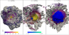 |
Fig. 1. Flame surface (gray) and density isosurfaces of ρ = 102, 103, 104, 105, 106, 107 g cm−3 (see colorbar) for model r60_d2.6. Left panel: situation prior to detonation initiation at t = 4.7 s. Middle panel: zoom in on the core at t = 4.78 s. The hotspot with temperatures above 1 × 10⁹ K is marked by the blue-green contour. Right panel: detonation front (blue surface) ∼1 s after initiation. The illustration is not to scale. |
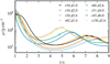 |
Fig. 2. Central density over time for a representative selection of models. The scatter points indicate the time of the detonation initiation. |
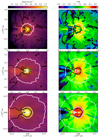 |
Fig. 3. Slices of the x − y-plane at z = 0 showing the density (left column) and the temperature (right column) of Model r10_d2.6 for three points in time: 6.21 s, 7.71 s and 8.31 s (from top to bottom). The white contour marks the zero level of the radial velocity, i.e., it separates regions of expansion and contraction and the black contour indicates X(CO) = 0.8. The blue point in the bottom left panel shows the location of the detonation initiation. |
We emphasize that although many of our simulations robustly ignite a detonation, this is not proof for the mechanism since the resolution in the area of interest is not fine enough to track the turbulent motions and shock waves inside the collision region (see Seitenzahl et al. 2009a) due to the expanding grid approach to track the ejecta. Moreover, we did not employ a reaction network in parallel with the hydrodynamics to capture the nuclear energy generation outside the flame. Therefore, the detonation location as well as tdet can be subject to slight variations within a specific model which may introduce some more diversity among the presented PGCD models. The energetic and nucleosynthesis yields as well as the synthetic observables of our simulations, however, are expected to largely capture the characteristics of these explosions.
5.2. Energetics and nucleosynthesis yields
The total nuclear energy Enuc released during the explosion is sufficient to unbind the whole WD in all simulations of this work. The disruption of the whole star was verified by checking that the kinetic energy of each cell exceeds its gravitational energy at the end of the simulations (t = 100 s). The ejecta expand homologously. While Enuc ranges from 1.61 to 1.96 × 1051 erg the energy released in the deflagration  lies between 1.29 and 3.15 × 1050 erg (see Table 1) which corresponds to 24.1 to 61.4% of the initial binding energy Ebind of the star. There is a clear trend that for an increasing deflagration strength (
 ) the time until detonation tdet increases and the central density ρdet at tdet, Enuc and with it the total kinetic energy Ekin decrease. This behavior is well in line with previous studies of the GCD scenario (see Sect. 1). A little scatter is added to these trends by the different initial central densities of the models. As an extreme example, Model r45_d6.0 and Model r82_d1.0 release a comparable amount of nuclear energy in the deflagration but differ significantly in their total energy release Enuc, and, especially in the amount of 56Ni produced. The high initial central density of Model r45_d6.0 also leads to a high value for ρdet of 8.8 × 10⁷ g cm−3 more than twice the value found for Model r82_d1.0. Moreover, the total amount of matter at high densities above 107 g cm−3 at the detonation initiation sums up to 0.98 M⊙ in Model r45_d6.0 and to 0.64 M⊙ in Model r82_d1.0, respectively.
The parameter driving the luminosity of SNe Ia is the mass of 56Ni ejected since it deposits energy into the expanding material via its decay to 56Co, and, subsequently, to 56Fe. The model sequence presented here covers a wide range of luminosities resulting from M(56Ni) ranging between 0.257 and 1.057 M⊙. This includes 56Ni masses appropriate for faint normal SNe Ia (see e.g. Stritzinger et al. 2006; Scalzo et al. 2014) but also the bright end of the SN Iax subclass (e.g., SN 2012Z ejecting ∼0.2 − 0.3 M⊙ of 56Ni and ∼MCh in total Stritzinger et al. 2015 or SN 2011ay Szalai et al. 2015) and 02es-like objects (see SN 2006bt also ejecting ∼0.2 − 0.3 M⊙ of 56Ni Foley et al. 2010). On the bright end, luminous normal SNe Ia, the slightly overluminous 91T-like objects (Filippenko et al. 1992) and the transitional events like SN 2000cx (Li et al. 2001) can also be accounted for by our models in terms of M(56Ni) ejected.
The result that models ignited at roff = 10 km do detonate pushes the transition between PGCDs and failed detonations, that is, pure deflagrations, to lower ignition radii compared to the works of Fisher & Jumper (2015) and Byrohl et al. (2019). These studies conclude that below ∼16 km a detonation initiation becomes unlikely, and, thus, the GCD mechanism produces mostly bright explosions. Indeed, the faintest model in our study, Model r10_d2.6, exhausts the viability of the PGCD mechanism since critical conditions for a detonation initiation are only reached at the very end of the contraction phase. However, subluminous SNe Ia resulting from the GCD scenario should still be considered rare events as pointed out by Byrohl et al. (2019). They extract a probability density function (PDF) for the ignition radius using data from Nonaka et al. (2012) to interpret their results. The PDF peaks at approximately 50 km and suggests that ignition below ∼20 km and above ∼100 km is a scarce event. In detail, they state that only 2.2% of MCh explosions are ignited below roff = 16 km.
Flörs et al. (2020) examine features of stable Ni, mostly in the form of 58Ni, and Fe in late-time spectra of SNe Ia. They then compare their measured Ni to Fe ratios (MNi/MFe) to theoretical models and conclude that most SNe Ia probably originate from sub-MCh WDs. In detail, they find that M58Ni/M56Ni < 6% for sub-MCh models (see references in Flörs et al. 2020) and larger for MCh explosions. The reason for this is that more neutron-rich isotopes are favored in nuclear statistical equilibrium at high densities which are reached in MCh WDs only. We find values of M58Ni/M56Ni between 2.4% and 5.1% making it hard to distinguish the PGCD models1 from sub-MCh explosions based on this ratio. Moreover, Flörs et al. (2020) state that M57Ni/M56Ni is expected to lie above 2% and M54, 56Fe/M56Ni above 10% for MCh models. Again, the nucleosynthesis yields of our simulations predict lower values of
M57Ni/M56Ni = 1.7 − 2.4% and M54, 56Fe/M56Ni = 1.8 − 14.6%. The obvious reason for this finding is that PGCD models exhibit characteristics of a deflagration at high densities and a detonation of a sub-MCh CO core. Finally, the significant amounts of IMEs produced in Model r10_d2.6 even exceed the mass of IGEs.
The elemental ratios to Fe compared to their solar value [X/Fe] (isotopes decayed to 2 Gyr) also include characteristics of both MCh deflagrations and detonations in low-mass WDs. First, supersolar values of [Mn/Fe] are achieved in models with a strong deflagration, for instance, Model r10_d2.6 and r10_d2.0 (see Fig. 4). This is in agreement with the commonly accepted fact that MCh explosions are responsible for a substantial amount of Mn in the Universe (Seitenzahl et al. 2013b; Lach et al. 2020). For decreasing deflagration strength the contribution of the detonation becomes larger and [Mn/Fe] falls below the solar value. Second, we observe high values of [Cr/Fe] in some explosions which is a direct imprint of low-mass (≲0.8 M⊙) CO detonation models (compare also Fig. 3 in Lach et al. 2020) but special for MCh models. Third, the usual overproduction of stable Ni in MCh deflagrations is suppressed by the detonation yields. Finally, Fig. 4 also shows signs of the strong odd-even effect in the detonation IME yields smoothed out by the deflagration products (compare again Fig. 3 in Lach et al. 2020). The α-elements Si, S, Ar and Ca are even synthesized in supersolar amounts in the core detonation of Model r10_d2.6. The rest of the models show rather low values of [α/Fe] more typical for MCh deflagrations. In summary, the nucleosynthesis yields of faint (r10_d2.6) to intermediately bright (r10_d2.0) models show characteristics of low-mass CO detonations as well as MCh explosions. As the deflagration strength decreases, the total elemental yields more and more resemble those of a pure CO detonation in a WD of approximately 1 M⊙. Nevertheless, the pollution of the outer layers with deflagration products still has some impact on the observables (see Sect. 6).
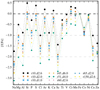 |
Fig. 4. Elemental abundances over Fe in relation to their solar value for a few representative models of the parameter study. |
5.3. Ejecta structure
The expelled material is spherically symmetric on large scales, especially the deflagration ashes which reach maximum velocities from ∼19 000 km s−1 (r10_d2.6, see Fig. 5) up to ∼29 000 km s−1 (r51_d4.0, see Fig. 6). The shell of well mixed deflagration products extends down to ∼8000 km s−1 in Model r10_d2.6 and ∼11 000 km s−1 for Model r51_d4.0. The outer boundary of the detonation products, primarily consisting of IMEs, is not exactly spherical but slightly elliptical and more elongated along the y-axis (perpendicular to the line connecting the deflagration and the detonation initiation). This structure is more pronounced in Model r82_d1.0 (see Fig. 7) and only very subtle in the most energetic explosion, that is, the strongest detonation, r51_d4.0. Moreover, the detonation region exhibits a cusp of deflagration products on the detonation side (left-hand side) disturbing the spherical structure. This is the region of the jet of ashes penetrating into the core until the detonation conditions are reached.
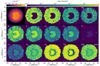 |
Fig. 5. Color-coded density and elemental abundance slices in the vx − vy-plane for Model r10_d2.6. |
A comparison of the ejecta structure to Fig. 4 of Seitenzahl et al. (2016) reveals an important difference: In their work the detonating core is not centered inside the deflagration ashes. This means that the envelope of burned material is thicker on the deflagration ignition side than on the detonation side leading to significant viewing angle effects. In our work the detonation products lie relatively well centered inside the shell of deflagration ashes (see Figs. 5–8). Only a very close inspection of Model r51_d4.0 (brightest) and Model r10_d2.6 (faintest) reveals that the deflagration envelope is slightly thicker on the deflagration side in Model r51_d4.0 than on the antipode. The opposite holds for Model r10_d2.6the deflagration envelope is slightly thicker on the deflagration side in Model r51_d4.0 than on the antipode. The opposite holds for Model r10_d2.6. In addition to this minor asymmetry, viewing angle effects can be expected to originate from the irregularly shaped core detonation. This difference between our models and the model of Seitenzahl et al. (2016) is very likely due to the distinct detonation initiation conditions. Since Seitenzahl et al. (2016) use optimistic values of ρ = 106 g cm−3 and T = 109 K the detonation is ignited very early (tdet = 2.37 s) almost immediately after the ashes have collided. Therefore, the amount of ashes on the detonation side has not piled up significantly and the detonation also ignites more off-center than found in this study. In our models the detonation only ignites after a prolonged period of contraction and the penetration of a jet into the core (tdet > 4.5 s) providing enough time for the deflagration products to engulf the core homogeneously.
The 1D-averaged velocity profiles of various elements and 56Ni are shown in Fig. 9 for a faint (r10_d2.6), a moderately bright (r10_d2.0) and an overluminous (r51_d3.0) model. All explosions are characterized by mixed deflagration products at high velocities dominated by 56Ni. The second most abundant elements are unburned C and O followed by Fe and Si. Less abundant IMEs present in the outer ejecta are S, Mg, and Ca while the mass fractions of Ar, Ti and Cr stay below 10−3. Going to lower velocities, the IMEs individually (from light to heavy) rise to a maximum and Fe and 56Ni exhibit a local minimum. This stratified region was burned in the detonation at rather low densities via incomplete silicon burning. The innermost regions are then dominated by 56Ni. The central density at detonation in Model r10_d2.6, however, is so low that even a significant fraction of IMEs is present at low velocities.
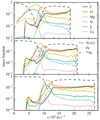 |
Fig. 9. 1D-averaged velocity profiles for C, O, Mg, Si, S, Ca, Ti+Cr, Fe and 56Ni. Upper panel: data for Model r10_d2.6, middle panel: Model r10_d2.0 and lower panel: Model r57_d3.0. |
From the ejecta structure it is evident that all of these models will display IGEs in their early-time spectra. This characteristic is in agreement with SNe Iax Foley et al. (2013), Jha (2017) as well as the overluminous 91T-like events. Normal SNe Ia, however, are dominated by IMEs around maximum light. Moreover, the fact that stable IGE are primarily found in the outer layers at high velocity neither matches the properties of 91T-like (Sasdelli et al. 2014; Seitenzahl et al. 2016) objects nor normal SNe Ia (Mazzali et al. 2007). The distribution of stable IGEs is also a problem for the method used in Flörs et al. (2020) (see also Sect. 5.2) to distinguish between MCh and sub-MCh mass models since only a small fraction of stable IGEs will be visible in late-time spectra.
6. Synthetic observables
To obtain synthetic spectra and light curves for our sequence of PGCD models we carried out time-dependent 3D Monte-Carlo RT simulations using the ARTIS code (Sim 2007; Kromer & Sim 2009). For each RT simulation we remapped the ejecta structure to a 503 grid. 108 photon packets were then tracked through the ejecta for 450 logarithmically spaced time steps between 0.1 and 100 days since explosion. We used the atomic data set described by Gall et al. (2012). We adopted a gray approximation in optically thick cells (cf. Kromer & Sim 2009) and for times earlier than 0.12 days post explosion local thermal equilibrium (LTE) is assumed. After this, we adopted our approximate NLTE description as presented by Kromer & Sim (2009). We calculated line of sight dependent light curves for 100 bins of equal solid-angle and line of sight dependent spectra for 10 different observer orientations of equal angle spacing that lie on the x − y-plane. The viewing angle dependent spectra we present here were calculated with the method described by Bulla et al. (2015) utilizing “virtual packets” leading to a significant reduction in the Monte-Carlo noise.
Figure 10 shows the bolometric and UBVRI band angle-averaged light curves for a selection of our PGCD models spanning from the faintest to the brightest model in our sequence. Observed light curves representing different subclasses of SNe Ia relevant for comparison to our model sequence are included for comparison: SN 1991T after which the luminous 91T-like subclass is named, SN 2011fe, a normal SN Ia and SN 2012Z, which is one of the bright members of the subluminous subclass of SNe Iax. We have shifted the explosion epochs of the observed light curves to better compare to the light curve evolution of the PGCD models. The explosion epochs we adopted are JD 2448359.5 for SN 1991T (2 days later than estimated by Filippenko et al. 1992), JD 2455800.2 for SN 2011fe (3 days later than estimated by Nugent et al. 2011) and JD 2455955.9 for SN 2012Z (2 days later than estimated by Yamanaka et al. 2015).
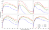 |
Fig. 10. Angle averaged bolometric and UBVRI band light curves for a subset of our PGCD models. Observed light curves representing different subclasses of SNe Ia are also included. SN 1991T (Lira et al. 1998), SN 2011fe (Richmond & Smith 2012; Tsvetkov et al. 2013; Munari et al. 2013; Brown et al. 2014; Stahl et al. 2019) and SN 2012Z (Stritzinger et al. 2015; Brown et al. 2014; Stahl et al. 2019). We made use of the Open Supernova Catalogue (Guillochon et al. 2017) to obtain the observed photometry. |
From Fig. 10 we can see that a feature of our PGCD model light curves is a relatively sharp initial rise over approximately the first 5 days post explosion (particularly in the U and B bands). After this, the light curves become quite flat and complex, with the exception of the faintest PGCD model r10_d2.6 (blue in Fig. 10), which shows an initial rapid decline post peak in the U and B bands. One of the intermediate brightness models shown in Fig. 10, Model r10_d1.0 (green), even exhibits a double peak in its U and B band light curves. This peculiar light curve behavior is driven by the interplay between the detonation ash at the center of the models and the deflagration ash which surrounds it. In all bands the radiation emitted from the decay of 56Ni in the deflagration ash dominates the initial rapid rise. However, as the band light curves approach peak, the contribution from the radiation emitted from the deflagration ash begins to diminish while the contribution of the radiation emitted from the detonation ash increases to become the dominant source of the luminosity for the band light curves. Such interplay between the deflagration and detonation ash distinguishes these PGCD models from pure detonation models (e.g., Sim et al. 2010; Blondin et al. 2017; Shen et al. 2018) and DD models (e.g., Gamezo et al. 2005; Röpke & Niemeyer 2007; Maeda et al. 2010b; Seitenzahl et al. 2013a).
It is clear from Fig. 10 that the best match is found between the band light curves of the brightest PGCD model in our sequence, Model r51_d4.0 (red) and SN 1991T. This is consistent with the results of Seitenzahl et al. (2016) who found the best match between their GCD model and SN 1991T. Model r51_d4.0 reproduces the initial rise of SN 1991T well in all bands until approximately 10 days post explosion with good agreement continuing to later times for certain bands. In particular, the model shows good agreement in B band with SN 1991T across all epochs shown. However, the band light curves of the model become too red as we move to later times. In particular, Model r51_d4.0 predicts a secondary peak that is approximately half a magnitude brighter than the first peak. A secondary peak of this size in I band is not observed for SN 1991T leading to a difference of over half a magnitude between the model and SN 1991T around the time of this secondary peak.
The band light curves of our PGCD models span a wide range of peak brightnesses (variations of almost 2 mag are predicted for the models in U, B and V bands). The models therefore cover a range of brightnesses which encompasses luminous SNe Ia such as those in the 91T-like subclass, normal SNe Ia and bright members of the subluminous SNe Iax class. However, the band light curves of our PGCD models show poor agreement with the normal SNe Ia, SN 2011fe and the bright SNe Iax, SN 2012Z in terms of colors and overall light curve evolution. Therefore, while we are able to reach lower brightnesses with our sequence compared to previous works the disagreement in the predicted light curves disfavors them as an explanation for either normal SNe Ia or SNe Iax.
From our light curve comparisons discussed above our PGCD models appear best suited to explain the 91T-like subclass (if any). In Fig. 11 we compare a selection of viewing angle dependent spectra, over a variety of epochs, for our brightest model (r51_d4.0, red), this is the model which produces best overall agreement in terms of light curves and spectra with SN 1991T. As was the case for the GCD model of Seitenzahl et al. (2016), our PGCD models are almost symmetric about the axis defined by the center of the star and the position of the initial deflagration ignition spark (located on the positive x-axis in Figs. 5–8). Therefore, we focus on different observer orientations that lie in the x − y-plane to demonstrate the viewing angle effects here. In Fig. 11 we identify these with ϕ, the angle made between the observer orientation and the x-axis. The ϕ = 0° direction corresponds to the observer viewing from the side where the initial deflagration spark was placed while the ϕ = 180° direction corresponds to the side where the detonation occurred. The viewing angles shown in Fig. 11 are representative of the range of brightness exhibited by this model depending on the line of sight. Model spectra are shown relative to explosion as labeled. As in Fig. 10 we adopted an explosion date of JD 2448359.5 for the SN 1991T spectra we compare to.
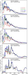 |
Fig. 11. Spectra over a variety of epochs for a selection of viewing angles for our brightest PGCD model (r51_d4.0). Observed spectra of SN 1991T (Ruiz-Lapuente et al. 1992; Phillips et al. 1992; Filippenko et al. 1992) are included for comparison. The observed spectra have been flux calibrated to match the photometry, dereddened using E(B − V) = 0.13 as estimated by Phillips et al. 1992) and deredshifted taking z = 0.006059 from interstellar Na. We take 30.76 as the distance modulus to SN 1991T (Saha et al. 2006). |
From Fig. 11 we can see that there are noticeable viewing angle variations in the spectra of Model r51_d4.0, for wavelengths of ∼5000 Å or less, at all epochs. This viewing angle dependency is driven by the asymmetric distribution of the deflagration ashes in the model that are rich in IGEs. As we can see from Fig. 6, which shows the ejecta structure of slices along the x − y-plane for Model r51_d4.0, the deflagration ashes extend over a greater range of velocities toward the side where the initial deflagration was ignited at ϕ = 0°, (positive x-axis in Fig. 6). This leads to increased line blanketing by IGEs for lines of sight looking close to this initial deflagration spark (e.g., ϕ = 0° spectra, red in Fig. 11), and, thus, the flux in the blue and UV is significantly reduced. The deflagration ashes, however, only cover a significantly greater velocity range for a relatively small window of viewing angles. Looking along ϕ = 72° (green in Fig. 11), we already see the line blanketing by IGEs in the blue and UV is significantly reduced and the flux at wavelengths less than ∼5000 Å is already quite similar to what is observed for the viewing angle looking toward where the detonation is first ignited (ϕ = 180°, blue in Fig. 11). Wavelengths greater than ∼5000 Å are less impacted by line blanketing due to IGEs, and, thus, do not show significant viewing angle dependencies. Additionally, as we move to later times, the viewing angle effects become less noticeable for the model as the outer layers become more optically thin. We find the same viewing angle dependency is observed in the B and U band light curves of Model r51_d4.0. The U band peak magnitudes vary between −19.5 to −20.5 while the B band peak magnitudes vary between −19.4 to −19.9. There is only very minimal viewing angle variation in the VRI band light curves. Overall, Model r51_d4.0 exhibits viewing angle dependencies comparable to those shown by the GCD model of Seitenzahl et al. (2016). Indeed, we find significant viewing angle dependencies for all of our models, with all models showing the largest viewing angle variation in the U and B bands. However, for fainter models the viewing angle variations in the VRI bands become increasingly prominent. We also find that the brightest and faintest viewing angles can correspond to significantly different observer orientations depending on the distribution of deflagration ash and differences between the irregularly shaped core detonations in each individual model.
The two brighter viewing angles shown in Fig. 11 (blue and green) show best spectroscopic agreement with SN 1991T, in particular at 9.1 and 12.9 days since explosion where they produce a good match to the overall flux of SN 1991T across all wavelengths. However, these viewing angles provide a poor match to the blue and UV flux at the earliest epoch shown and also have significantly too much flux in the red wavelengths for the last two epochs shown. Therefore, although promising, we find no individual viewing angles which provide a consistently good match to the spectra of SN 1991T over multiple epochs. Additionally, as noted above and already found for the GCD model of Seitenzahl et al. (2016), none of the PGCD models produce good spectroscopic agreement with normal SNe Ia, showing IME features which are too weak and spectra which are too red particularly toward later epochs.
As we have discussed above the band light curves of the faintest PGCD model in our sequence do not produce good agreement with those of bright SNe Iax such as SN 2012Z. However, our faintest model has a brightness similar to bright SNe Iax. As 91T-like SNe Ia and SNe Iax are known to be spectroscopically similar before peak and a more stratified ejecta structure as opposed to pure deflagration models is suggested for bright SNe Iax (Barna et al. 2017; Stritzinger et al. 2015) we briefly explore the spectroscopic comparisons between our faintest PGCD model and the bright SN Iax, SN 2012Z. In particular, we investigated whether our PGCD model spectra might compare more favorably than the pure deflagration models of L21. Figure 12 shows spectroscopic comparisons between the bright SN Iax, SN 2012Z, the angle-averaged spectra for our faintest PGCD model (r10_d2.6, red) and the brightest model in our sequence of pure deflagration models from L21 (r10_d4.0_Z, blue). We compare these models to SN 2012Z as they are the models from each sequence that match the brightness of SN 2012Z most closely. From Fig. 12 we see that the spectra of our PGCD and pure deflagration models show significantly different flux in both the epochs shown as well as a different evolution in their flux between the two epochs. However, they do predict many of the same spectral features, although the line velocities of these features are noticeably more blue shifted for our PGCD model. This is to be expected as the PGCD model is more energetic than the pure deflagration model leading to higher ejecta velocities. For the earlier epoch shown (8.1 days since explosion) the pure deflagration model (blue) shows better spectroscopic agreement with SN 2012Z as it matches the overall flux profile of SN 2012Z much better. At this epoch our PGCD model (red) shows a large amount of emission between ∼5000 to 6000 Å as a result of the re-emission of radiation absorbed by IGEs in the UV. This is not observed in the spectrum of SN 2012Z at this epoch. For the later spectra shown (22.7 days post explosion) the PGCD model shows better overall flux agreement with the spectra of SN 2012Z than the deflagration model. This is because the deflagration model is too fast in decline compared to SN 2012Z which is a general issue that is encountered when we compare pure deflagration models to SNe Iax (see L21 for more details). However, the deflagration model reproduces the locations of individual spectral features of SN 2012Z at least as successfully as the PGCD model and in particular provides a better match for the location of the Ca II infrared triplet than the PGCD model. Previous work, presented by L21, has also shown that we are able to produce reasonably good spectroscopic and light curve agreement with intermediate luminosity SNe Iax using our sequence of pure deflagration models. However, none of our PGCD models presented here are faint enough to produce agreement with intermediate luminosity SNe Iax. Therefore, our pure deflagration models do appear more promising to explain SNe Iax than our PGCD models.
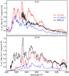 |
Fig. 12. Spectroscopic comparisons between the bright SN Iax, SN 2012Z (Stritzinger et al. 2015), along with angle-averaged spectra for our faintest PGCD model (r10_d2.6, red) and the brightest pure deflagration model from our previous pure deflagration study, L21 (r10_d4.0_Z, blue). Times displayed are relative to explosion for all spectra. We take the explosion time estimated for SN 2012Z by Yamanaka et al. (2015). The observed spectra of SN 2012Z have been flux calibrated to match the photometry. Additionally, they have been corrected for distance, red shift and reddening assuming a distance of 33.0 Mpc, z = 0.007125 and E(B − V) = 0.11 (Stritzinger et al. 2015). |
7. Conclusions
We used the pure deflagration simulations of L21 as initial models for a parameter study of the GCD scenario containing 11 models. The initial models used in this work were ignited in a single spark off-center at varying radii roff between 10 and 150 km. Moreover, different central densities of ρc = 1, 2, 2.6, 3, 4, 5, 6 × 10⁹ g cm−3 were explored. The suite of models presented here constitutes one of the largest systematic studies of the GCD scenario to date.
Our explosions proceed similar to the models presented in earlier works (Plewa et al. 2004; Plewa 2007; Townsley et al. 2007; Röpke et al. 2007; Jordan et al. 2008; Meakin et al. 2009; Seitenzahl et al. 2016), and Byrohl et al. (2019): The deflagration front burns toward the surface, burned ashes spread around the WD and collide at the opposite side of the star. This collision produces an inwardly directed jet which compresses and heats material ahead and leads to the initiation of a detonation. In the case of our models, this compression is aided by the coincidence of the first pulsation phase of the WD and the collision of the ashes, and, thus, our models resemble the “pulsationally assisted gravitationally confined detonation” scenario presented by Jordan et al. (2012b).
We find that all but the most energetic models from L21 satisfy the conditions for a detonation, that is, they simultaneously reach values of ρcrit > 1 × 10⁷ g cm−3 and Tcrit > 2 × 10⁹ K in one grid cell. Moreover, we can corroborate the results of García-Senz et al. (2016) who state that rotation disturbs the focus of the collision, and, therefore, suppresses the initiation of a detonation in the GCD mechanism. In addition, the combination of different central densities and ignition locations introduces some diversity to the inverse proportionality of deflagration strength and synthesized mass of 56Ni.
The set of models produces a wide range of 56Ni masses, that is, brightnesses, from 1.057 down to 0.257 M⊙ which is the faintest GCD model published to date. This range comprises the subluminous SNe Iax, normal SNe Ia as well as the slightly overluminous 91T-like objects. We also study, inspired by Flörs et al. (2020), the ratio of stable IGEs to 56Ni in the ejecta and find that the GCD scenario blurs the boundaries between typical nucleosynthesis products of the sub-MCh and MCh scenario. Since our models contain a deflagration as well as a detonation a mixture of characteristics of both channels is reasonable. The same holds for the [Mn/Fe] value which ranges from subsolar to supersolar values. (Detailed nucleosynthesis yields will be published on HESMA (Kromer et al. 2017) as will the angle-averaged optical spectral time series and UVOIR bolometric light curves calculated in the radiative transfer simulations).
Furthermore, the UBVRI band light curves show a complex evolution reflecting the transition to a detonation at various states of the pre-expanded WD core. We compare model light curves to the bright SN 1991T, the normal event SN 2011fe and the SN Iax SN 2012Z finding that only SN 1991T can be reproduced for early times up to 10 d after explosion. At later epochs (≳20 d), the light curves exhibit an unusually prominent secondary maximum. The B band, however, shows good agreement with SN 1991T at all times. While there is still some disagreement between observations and models the GCD or PGCD scenario is still the most promising scenario for 91T-like SNe presented to date.
We also report a strong viewing angle dependency (our analysis presented here focuses on the brightest model in the sequence) showing line blanketing due to the prominent deflagration ashes on the ignition side, and, hence, a suppressed flux at blue wavelengths below ∼5000 Å. A spectral comparison to SN 1991T reveals that good agreement is only found for intermediate times (9.1 and 12.9 d after explosion) for viewing angles away from the deflagration ignition spot. For late times, however, these viewing angle dependencies vanish since the detonation products dominate the spectra.
Despite the poor agreement of the light curve evolution, we compared the spectra of the faintest model in the study to SN 2012Z. In addition, we add the brightest pure deflagration model of L21 and conclude that deflagrations still provide a better match to these transients and that SNe Iax are most probably not the result of the GCD scenario.
Since our simulations are not able to predict whether a detonation is really initiated we speculate that SNe Iax and 91T-like SNe might originate from the same progenitor system. In the case of a failed detonation (more likely for strong deflagrations) a SN Iax arises and in the case of a successful detonation (more likely for weak deflagrations) the result is a 91T-like transient. This is a reasonable explanation for their similar spectra near maximum light and their very different luminosity and post-maximum evolution. It should be noted that the ignition of a deflagration in a MCh WD is a stochastic process, and that strong deflagrations resulting from an ignition near the center can be considered a rare event (Nonaka et al. 2012; Byrohl et al. 2019). However, more simmering phase simulations with different WD models are still needed to validate the findings of Nonaka et al. (2012). Finally, although our fainter models do not reproduce any observations of SNe Ia, these might still occur in nature as rare events not detected to date and they could be identified due to their characteristic observables.
The full set of isotopic yields and also the angle averaged optical spectral time series and UVOIR bolometric light curves calculated in the radiative transfer simulations will be published on HESMA Kromer et al. (2017).
Acknowledgments
This work was supported by the Deutsche Forschungsgemeinschaft (DFG, German Research Foundation) – Project-ID 138713538 – SFB 881 (“The Milky Way System”, subproject A10), by the ChETEC COST Action (CA16117), and by the National Science Foundation under Grant No. OISE-1927130 (IReNA). FL and FKR acknowledge support by the Klaus Tschira Foundation. FPC acknowledges an STFC studentship and SAS acknowledges funding from STFC Grant Ref: ST/P000312/1. NumPy and SciPy (Oliphant 2007), IPython (Pérez & Granger 2007), and Matplotlib (Hunter 2007) were used for data processing and plotting. The authors gratefully acknowledge the Gauss Centre for Supercomputing e.V. (www.gauss-centre.eu) for funding this project by providing computing time on the GCS Supercomputer JUWELS (Jülich Supercomputing Centre 2019) at Jülich Supercomputing Centre (JSC). Part of this work was performed using the Cambridge Service for Data Driven Discovery (CSD3), part of which is operated by the University of Cambridge Research Computing on behalf of the STFC DiRAC HPC Facility (www.dirac.ac.uk). The DiRAC component of CSD3 was funded by BEIS capital funding via STFC capital grants ST/P002307/1 and ST/R002452/1 and STFC operations grant ST/R00689X/1. DiRAC is part of the National e-Infrastructure. We thank James Gillanders for assisting with the flux calibrations of the observed spectra.
References
- Arnett, W. D. 1969, Ap&SS, 5, 180 [NASA ADS] [CrossRef] [Google Scholar]
- Barna, B., Szalai, T., Kromer, M., et al. 2017, MNRAS, 471, 4865 [NASA ADS] [CrossRef] [Google Scholar]
- Baron, E., Jeffery, D. J., Branch, D., et al. 2008, ApJ, 672, 1038 [NASA ADS] [CrossRef] [Google Scholar]
- Blondin, S., Dessart, L., Hillier, D. J., & Khokhlov, A. M. 2013, MNRAS, 429, 2127 [NASA ADS] [CrossRef] [Google Scholar]
- Blondin, S., Dessart, L., Hillier, D. J., & Khokhlov, A. M. 2017, MNRAS, 470, 157 [Google Scholar]
- Branch, D., Baron, E., Thomas, R. C., et al. 2004, PASP, 116, 903 [NASA ADS] [CrossRef] [Google Scholar]
- Bravo, E., & García-Senz, D. 2006, ApJ, 642, L157 [NASA ADS] [CrossRef] [Google Scholar]
- Bravo, E., & García-Senz, D. 2009, ApJ, 695, 1244 [NASA ADS] [CrossRef] [Google Scholar]
- Bravo, E., García-Senz, D., Cabezón, R. M., & Domínguez, I. 2009, ApJ, 695, 1257 [NASA ADS] [CrossRef] [Google Scholar]
- Bravo, E., Gil-Pons, P., Gutiérrez, J. L., & Doherty, C. L. 2016, A&A, 589, A38 [NASA ADS] [CrossRef] [EDP Sciences] [Google Scholar]
- Brown, P. J., Breeveld, A. A., Holland, S., Kuin, P., & Pritchard, T. 2014, Ap&SS, 354, 89 [Google Scholar]
- Bulla, M., Sim, S. A., & Kromer, M. 2015, MNRAS, 450, 967 [Google Scholar]
- Byrohl, C., Fisher, R., & Townsley, D. 2019, ApJ, 878, 67 [NASA ADS] [CrossRef] [Google Scholar]
- Colella, P., & Woodward, P. R. 1984, J. Comput. Phys., 54, 174 [NASA ADS] [CrossRef] [Google Scholar]
- Denissenkov, P. A., Truran, J. W., Herwig, F., et al. 2015, MNRAS, 447, 2696 [NASA ADS] [CrossRef] [Google Scholar]
- Dessart, L., Blondin, S., Hillier, D. J., & Khokhlov, A. 2014, MNRAS, 441, 532 [NASA ADS] [CrossRef] [Google Scholar]
- Dursi, L. J., & Timmes, F. X. 2006, ApJ, 641, 1071 [NASA ADS] [CrossRef] [Google Scholar]
- Filippenko, A. V., Richmond, M. W., Matheson, T., et al. 1992, ApJ, 384, L15 [CrossRef] [Google Scholar]
- Fink, M., Kromer, M., Seitenzahl, I. R., et al. 2014, MNRAS, 438, 1762 [NASA ADS] [CrossRef] [Google Scholar]
- Fisher, R., & Jumper, K. 2015, ApJ, 805, 150 [NASA ADS] [CrossRef] [Google Scholar]
- Flörs, A., Spyromilio, J., Taubenberger, S., et al. 2020, MNRAS, 491, 2902 [NASA ADS] [Google Scholar]
- Foley, R. J., Narayan, G., Challis, P. J., et al. 2010, ApJ, 708, 1748 [NASA ADS] [CrossRef] [Google Scholar]
- Foley, R. J., Challis, P. J., Chornock, R., et al. 2013, ApJ, 767, 57 [Google Scholar]
- Gall, E. E. E., Taubenberger, S., Kromer, M., et al. 2012, MNRAS, 427, 994 [NASA ADS] [CrossRef] [Google Scholar]
- Gamezo, V. N., Khokhlov, A. M., & Oran, E. S. 2005, ApJ, 623, 337 [NASA ADS] [CrossRef] [Google Scholar]
- García-Senz, D., Cabezón, R. M., Domínguez, I., & Thielemann, F. K. 2016, ApJ, 819, 132 [CrossRef] [Google Scholar]
- Guillochon, J., Parrent, J., Kelley, L. Z., & Margutti, R. 2017, ApJ, 835, 64 [Google Scholar]
- Hillebrandt, W., Kromer, M., Röpke, F. K., & Ruiter, A. J. 2013, Front. Phys., 8, 116 [Google Scholar]
- Höflich, P., Khokhlov, A., & Wheeler, J. 1995, ApJ, 444, 831 [CrossRef] [Google Scholar]
- Hoyle, F., & Fowler, W. A. 1960, ApJ, 132, 565 [NASA ADS] [CrossRef] [Google Scholar]
- Hunter, J. D. 2007, Comput. Sci. Eng., 9, 90 [NASA ADS] [CrossRef] [Google Scholar]
- Iben, I., Jr., & Tutukov, A. V. 1984, ApJS, 54, 335 [NASA ADS] [CrossRef] [Google Scholar]
- Jha, S. W. 2017, in Handbook of Supernovae, (Springer) 375 [CrossRef] [Google Scholar]
- Jordan, G. C., IV, Fisher, R. T., Townsley, D. M., et al. 2008, ApJ, 681, 1448 [NASA ADS] [CrossRef] [Google Scholar]
- Jordan, G. C., Meakin, C. A., Hearn, N., et al. 2009, in Numerical Modeling of Space Plasma Flows: ASTRONUM-2008, eds. N. V. Pogorelov, E. Audit, P. Colella, & G. P. Zank, ASP Conf. Ser., 406, 92 [Google Scholar]
- Jordan, G. C., IV, Graziani, C., Fisher, R. T., et al. 2012a, ApJ, 759, 53 [NASA ADS] [CrossRef] [Google Scholar]
- Jordan, G. C., IV, Perets, H. B., Fisher, R. T., & van Rossum, D. R. 2012b, ApJ, 761, L23 [NASA ADS] [CrossRef] [Google Scholar]
- Jülich Supercomputing Centre 2019, Journal of Large-scale Research Facilities, 5, A171 [Google Scholar]
- Kasen, D., & Plewa, T. 2005, ApJ, 622, L41 [NASA ADS] [CrossRef] [Google Scholar]
- Kasen, D., & Plewa, T. 2007, ApJ, 662, 459 [NASA ADS] [CrossRef] [Google Scholar]
- Kasen, D., Röpke, F. K., & Woosley, S. E. 2009, Nature, 460, 869 [Google Scholar]
- Kashyap, R., Haque, T., Lorén-Aguilar, P., García-Berro, E., & Fisher, R. 2018, ApJ, 869, 140 [NASA ADS] [CrossRef] [Google Scholar]
- Khokhlov, A. M. 1991, A&A, 245, L25 [NASA ADS] [Google Scholar]
- Khokhlov, A., Mueller, E., & Hoeflich, P. 1993, A&A, 270, 223 [NASA ADS] [CrossRef] [Google Scholar]
- Khokhlov, A. M., Oran, E. S., & Wheeler, J. C. 1997, ApJ, 478, 678 [Google Scholar]
- Kromer, M., & Sim, S. A. 2009, MNRAS, 398, 1809 [Google Scholar]
- Kromer, M., Fink, M., Stanishev, V., et al. 2013, MNRAS, 429, 2287 [NASA ADS] [CrossRef] [Google Scholar]
- Kromer, M., Ohlmann, S. T., Pakmor, R., et al. 2015, MNRAS, 450, 3045 [NASA ADS] [CrossRef] [Google Scholar]
- Kromer, M., Ohlmann, S. T., & Roepke, F. K. 2017, Mem. Soc. Astron. It., 88, 312 [Google Scholar]
- Lach, F., Röpke, F. K., Seitenzahl, I. R., et al. 2020, A&A, 644, A118 [NASA ADS] [CrossRef] [EDP Sciences] [Google Scholar]
- Lach, F., Callan, F. P., Bubeck, D., et al. 2022, A&A, 658, A179 [NASA ADS] [CrossRef] [EDP Sciences] [Google Scholar]
- Li, W., Filippenko, A. V., Treffers, R. R., et al. 2001, ApJ, 546, 734 [NASA ADS] [CrossRef] [Google Scholar]
- Lira, P., Suntzeff, N. B., Phillips, M. M., et al. 1998, AJ, 115, 234 [NASA ADS] [CrossRef] [Google Scholar]
- Long, M., Jordan, G. C., IV, Van Rossum, D. R., et al. 2014, ApJ, 789, 103 [NASA ADS] [CrossRef] [Google Scholar]
- Maeda, K., Taubenberger, S., Sollerman, J., et al. 2010a, ApJ, 708, 1703 [NASA ADS] [CrossRef] [Google Scholar]
- Maeda, K., Röpke, F. K., Fink, M., et al. 2010b, ApJ, 712, 624 [CrossRef] [Google Scholar]
- Marquardt, K. S., Sim, S. A., Ruiter, A. J., et al. 2015, A&A, 580, A118 [NASA ADS] [CrossRef] [EDP Sciences] [Google Scholar]
- Mazzali, P. A., Röpke, F. K., Benetti, S., & Hillebrandt, W. 2007, Science, 315, 825 [NASA ADS] [CrossRef] [Google Scholar]
- Meakin, C. A., Seitenzahl, I., Townsley, D., et al. 2009, ApJ, 693, 1188 [NASA ADS] [CrossRef] [Google Scholar]
- Munari, U., Henden, A., Belligoli, R., et al. 2013, New Astron., 20, 30 [Google Scholar]
- Niemeyer, J. C., & Woosley, S. E. 1997, ApJ, 475, 740 [NASA ADS] [CrossRef] [Google Scholar]
- Nomoto, K., Thielemann, F.-K., & Yokoi, K. 1984, ApJ, 286, 644 [NASA ADS] [CrossRef] [Google Scholar]
- Nonaka, A., Aspden, A. J., Zingale, M., et al. 2012, ApJ, 745, 73 [NASA ADS] [CrossRef] [Google Scholar]
- Nugent, P. E., Sullivan, M., Cenko, S. B., et al. 2011, Nature, 480, 344 [NASA ADS] [CrossRef] [Google Scholar]
- Oliphant, T. E. 2007, Comput. Sci. Eng., 9, 10 [NASA ADS] [CrossRef] [Google Scholar]
- Oran, E. S., & Gamezo, V. N. 2007, Combust. Flame, 148, 4 [Google Scholar]
- Pakmor, R., Edelmann, P., Röpke, F. K., & Hillebrandt, W. 2012, MNRAS, 424, 2222 [Google Scholar]
- Pakmor, R., Zenati, Y., Perets, H. B., & Toonen, S. 2021, MNRAS, 503, 4734 [Google Scholar]
- Pérez, F., & Granger, B. E. 2007, Comput. Sci. Eng., 9, 21 [Google Scholar]
- Phillips, M. M. 1993, ApJ, 413, L105 [Google Scholar]
- Phillips, M. M., Wells, L. A., Suntzeff, N. B., et al. 1992, AJ, 103, 1632 [NASA ADS] [CrossRef] [Google Scholar]
- Phillips, M. M., Li, W., Frieman, J. A., et al. 2007, PASP, 119, 360 [CrossRef] [Google Scholar]
- Plewa, T. 2007, ApJ, 657, 942 [NASA ADS] [CrossRef] [Google Scholar]
- Plewa, T., Calder, A. C., & Lamb, D. Q. 2004, ApJ, 612, L37 [Google Scholar]
- Poludnenko, A. Y., Gardiner, T. A., & Oran, E. S. 2011, Phys. Rev. Lett., 107, 054501 [NASA ADS] [CrossRef] [Google Scholar]
- Poludnenko, A. Y., Chambers, J., Ahmed, K., Gamezo, V. N., & Taylor, B. D. 2019, Science, 366, 7365 [NASA ADS] [CrossRef] [Google Scholar]
- Richmond, M. W., & Smith, H. A. 2012, J. Am. Assoc. Var. Star, 40, 872 [NASA ADS] [Google Scholar]
- Röpke, F. K. 2005, A&A, 432, 969 [NASA ADS] [CrossRef] [EDP Sciences] [Google Scholar]
- Röpke, F. K. 2016, in Handbook of Supernovae, eds. A. Alsabti, & P. Murdin (Springer), 1185 [Google Scholar]
- Röpke, F. K., & Niemeyer, J. C. 2007, A&A, 464, 683 [NASA ADS] [CrossRef] [EDP Sciences] [Google Scholar]
- Röpke, F. K., Woosley, S. E., & Hillebrandt, W. 2007, ApJ, 660, 1344 [Google Scholar]
- Ruiz-Lapuente, P., Cappellaro, E., Turatto, M., et al. 1992, ApJ, 387, L33 [NASA ADS] [CrossRef] [Google Scholar]
- Saha, A., Thim, F., Tammann, G. A., Reindl, B., & Sandage, A. 2006, ApJS, 165, 108 [Google Scholar]
- Sasdelli, M., Mazzali, P. A., Pian, E., et al. 2014, MNRAS, 445, 711 [NASA ADS] [CrossRef] [Google Scholar]
- Scalzo, R., Aldering, G., Antilogus, P., et al. 2014, MNRAS, 440, 1498 [NASA ADS] [CrossRef] [Google Scholar]
- Seitenzahl, I. R., Meakin, C. A., Townsley, D. M., Lamb, D. Q., & Truran, J. W. 2009a, ApJ, 696, 515 [Google Scholar]
- Seitenzahl, I. R., Meakin, C. A., Lamb, D. Q., & Truran, J. W. 2009b, ApJ, 700, 642 [NASA ADS] [CrossRef] [Google Scholar]
- Seitenzahl, I. R., Ciaraldi-Schoolmann, F., Röpke, F. K., et al. 2013a, MNRAS, 429, 1156 [NASA ADS] [CrossRef] [Google Scholar]
- Seitenzahl, I. R., Cescutti, G., Röpke, F. K., Ruiter, A. J., & Pakmor, R. 2013b, A&A, 559, L5 [NASA ADS] [CrossRef] [EDP Sciences] [Google Scholar]
- Seitenzahl, I. R., Kromer, M., Ohlmann, S. T., et al. 2016, A&A, 592, A57 [NASA ADS] [CrossRef] [EDP Sciences] [Google Scholar]
- Sethian, J. A. 1999, Level Set Methods and Fast Marching Methods (Cambride: Cambridge University Press) [Google Scholar]
- Shen, K. J., Kasen, D., Miles, B. J., & Townsley, D. M. 2018, ApJ, 854, 52 [Google Scholar]
- Shen, K. J., Blondin, S., Kasen, D., et al. 2021, ApJ, 909, L18 [NASA ADS] [CrossRef] [Google Scholar]
- Sim, S. A. 2007, MNRAS, 375, 154 [NASA ADS] [CrossRef] [Google Scholar]
- Sim, S. A., Röpke, F. K., Hillebrandt, W., et al. 2010, ApJ, 714, L52 [Google Scholar]
- Sim, S. A., Seitenzahl, I. R., Kromer, M., et al. 2013, MNRAS, 436, 333 [Google Scholar]
- Stahl, B. E., Zheng, W., de Jaeger, T., et al. 2019, MNRAS, 490, 3882 [NASA ADS] [CrossRef] [Google Scholar]
- Stritzinger, M., Mazzali, P. A., Sollerman, J., & Benetti, S. 2006, A&A, 460, 793 [NASA ADS] [CrossRef] [EDP Sciences] [Google Scholar]
- Stritzinger, M. D., Valenti, S., Hoeflich, P., et al. 2015, A&A, 573, A2 [NASA ADS] [CrossRef] [EDP Sciences] [Google Scholar]
- Szalai, T., Vinkó, J., Sárneczky, K., et al. 2015, MNRAS, 453, 2103 [NASA ADS] [CrossRef] [Google Scholar]
- Taubenberger, S. 2017, Handbook of Supernovae, 317 [CrossRef] [Google Scholar]
- Timmes, F. X., & Arnett, D. 1999, ApJS, 125, 277 [Google Scholar]
- Townsley, D. M., Calder, A. C., Asida, S. M., et al. 2007, ApJ, 668, 1118 [NASA ADS] [CrossRef] [Google Scholar]
- Travaglio, C., Hillebrandt, W., Reinecke, M., & Thielemann, F.-K. 2004, A&A, 425, 1029 [NASA ADS] [CrossRef] [EDP Sciences] [Google Scholar]
- Tsvetkov, D. Y., Shugarov, S. Y., Volkov, I. M., et al. 2013, Contrib. Astron. Obs. Skaln. Pleso, 43, 94 [NASA ADS] [Google Scholar]
- Whelan, J., & Iben, I., Jr. 1973, ApJ, 186, 1007 [Google Scholar]
- Woosley, S. E., Kerstein, A. R., Sankaran, V., Aspden, A. J., & Röpke, F. K. 2009, ApJ, 704, 255 [NASA ADS] [CrossRef] [Google Scholar]
- Yamanaka, M., Maeda, K., Kawabata, K. S., et al. 2015, ApJ, 806, 191 [NASA ADS] [CrossRef] [Google Scholar]
- Zel’dovich, Y. B., Librovich, V. B., Makhviladze, G. M., & Sivashinskii, G. I. 1970, J. Appl. Mech. Tech. Phys., 11, 264 [Google Scholar]
- Zingale, M., Almgren, A. S., Bell, J. B., Nonaka, A., & Woosley, S. E. 2009, ApJ, 704, 196 [NASA ADS] [CrossRef] [Google Scholar]
- Zingale, M., Nonaka, A., Almgren, A. S., et al. 2011, ApJ, 740, 8 [NASA ADS] [CrossRef] [Google Scholar]
All Tables
Summary of the main properties of the ejected material and the initial conditions.
All Figures
|
Fig. 1. Flame surface (gray) and density isosurfaces of ρ = 102, 103, 104, 105, 106, 107 g cm−3 (see colorbar) for model r60_d2.6. Left panel: situation prior to detonation initiation at t = 4.7 s. Middle panel: zoom in on the core at t = 4.78 s. The hotspot with temperatures above 1 × 10⁹ K is marked by the blue-green contour. Right panel: detonation front (blue surface) ∼1 s after initiation. The illustration is not to scale. |
| In the text | |
|
Fig. 2. Central density over time for a representative selection of models. The scatter points indicate the time of the detonation initiation. |
| In the text | |
|
Fig. 3. Slices of the x − y-plane at z = 0 showing the density (left column) and the temperature (right column) of Model r10_d2.6 for three points in time: 6.21 s, 7.71 s and 8.31 s (from top to bottom). The white contour marks the zero level of the radial velocity, i.e., it separates regions of expansion and contraction and the black contour indicates X(CO) = 0.8. The blue point in the bottom left panel shows the location of the detonation initiation. |
| In the text | |
|
Fig. 4. Elemental abundances over Fe in relation to their solar value for a few representative models of the parameter study. |
| In the text | |
|
Fig. 5. Color-coded density and elemental abundance slices in the vx − vy-plane for Model r10_d2.6. |
| In the text | |
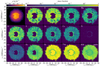 |
Fig. 6. Same as Fig. 5, but for Model r51_d4.0. |
| In the text | |
 |
Fig. 7. Same as Fig. 5, but for Model r82_d1.0. |
| In the text | |
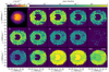 |
Fig. 8. Same as Fig. 5, but for Model r60_d2.6. |
| In the text | |
|
Fig. 9. 1D-averaged velocity profiles for C, O, Mg, Si, S, Ca, Ti+Cr, Fe and 56Ni. Upper panel: data for Model r10_d2.6, middle panel: Model r10_d2.0 and lower panel: Model r57_d3.0. |
| In the text | |
|
Fig. 10. Angle averaged bolometric and UBVRI band light curves for a subset of our PGCD models. Observed light curves representing different subclasses of SNe Ia are also included. SN 1991T (Lira et al. 1998), SN 2011fe (Richmond & Smith 2012; Tsvetkov et al. 2013; Munari et al. 2013; Brown et al. 2014; Stahl et al. 2019) and SN 2012Z (Stritzinger et al. 2015; Brown et al. 2014; Stahl et al. 2019). We made use of the Open Supernova Catalogue (Guillochon et al. 2017) to obtain the observed photometry. |
| In the text | |
|
Fig. 11. Spectra over a variety of epochs for a selection of viewing angles for our brightest PGCD model (r51_d4.0). Observed spectra of SN 1991T (Ruiz-Lapuente et al. 1992; Phillips et al. 1992; Filippenko et al. 1992) are included for comparison. The observed spectra have been flux calibrated to match the photometry, dereddened using E(B − V) = 0.13 as estimated by Phillips et al. 1992) and deredshifted taking z = 0.006059 from interstellar Na. We take 30.76 as the distance modulus to SN 1991T (Saha et al. 2006). |
| In the text | |
|
Fig. 12. Spectroscopic comparisons between the bright SN Iax, SN 2012Z (Stritzinger et al. 2015), along with angle-averaged spectra for our faintest PGCD model (r10_d2.6, red) and the brightest pure deflagration model from our previous pure deflagration study, L21 (r10_d4.0_Z, blue). Times displayed are relative to explosion for all spectra. We take the explosion time estimated for SN 2012Z by Yamanaka et al. (2015). The observed spectra of SN 2012Z have been flux calibrated to match the photometry. Additionally, they have been corrected for distance, red shift and reddening assuming a distance of 33.0 Mpc, z = 0.007125 and E(B − V) = 0.11 (Stritzinger et al. 2015). |
| In the text | |
Current usage metrics show cumulative count of Article Views (full-text article views including HTML views, PDF and ePub downloads, according to the available data) and Abstracts Views on Vision4Press platform.
Data correspond to usage on the plateform after 2015. The current usage metrics is available 48-96 hours after online publication and is updated daily on week days.
Initial download of the metrics may take a while.