| Issue |
A&A
Volume 659, March 2022
|
|
|---|---|---|
| Article Number | A114 | |
| Number of page(s) | 27 | |
| Section | Planets and planetary systems | |
| DOI | https://doi.org/10.1051/0004-6361/202141468 | |
| Published online | 15 March 2022 | |
Investigating the detectability of hydrocarbons in exoplanet atmospheres with JWST★
1
Institute of Astronomy, KU Leuven,
Celestijnenlaan 200D,
3001
Leuven,
Belgium
e-mail: This email address is being protected from spambots. You need JavaScript enabled to view it.
2
SRON Netherlands Institute for Space Research,
Sorbonnelaan 2,
3584 CA,
Utrecht, The Netherlands
3
Centre for Exoplanet Science, University of St Andrews,
Nort Haugh,
St Andrews,
KY169SS, UK
e-mail: This email address is being protected from spambots. You need JavaScript enabled to view it.
Received:
4
June
2021
Accepted:
7
January
2022
Abstract
Aims. We investigate at what abundances various hydrocarbon molecules (e.g. acetylene (C2H2), ethylene (C2H4), and methane (CH4)) become detectable when observing the atmospheres of various planets using the James Webb Space Telescope (JWST).
Methods. We focused on atmospheric models based on the parameters of a small sample of planets: HD 189733b, HD 209458b (hot Jupiters orbiting bright stars); HD 97658b (a sub-Neptune/super-Earth orbiting a bright star); and Kepler-30c (a warm Jupiter orbiting a faint star). We computed model transmission spectra, assuming equilibrium chemistry and clear atmospheres for all planets apart from HD 189733b, where we also computed spectra with a moderate cloud layer included. We used the Bayesian retrieval package ARCiS for the model atmospheres, and simulated observed spectra from different instruments that will be on board JWST using the PandExo package. We subsequently ran retrievals on these spectra to determine whether the parameters input into the forward models, with a focus on molecular abundances, can be accurately retrieved from these simulated spectra.
Results. We find that generally we can detect and retrieve abundances of the hydrocarbon species as long as they have a volume mixing ratio above approximately 1 × 10⁻⁷–1 × 10⁻⁶, at least for the brighter targets. There are variations based on planet type and instrument(s) used, and these limits will likely change depending on the abundance of other strong absorbers. We also find scenarios where the presence of one hydrocarbon is confused with another, particularly when a small wavelength region is covered; this is often improved when two instruments are combined.
Conclusions. The molecules C2H2, CH4, and C2H4 will all be detectable with JWST, provided they are present in high enough abundances, and that the optimal instruments are chosen for the exoplanet system being observed. Our results indicate that generally a combination of two instruments, either NIRSpec G395M and MIRI LRS, or NIRCam F322W2 and MIRI LRS, are best for observing these hydrocarbons in bright exoplanet systems with planets of various sizes, with NIRSpec G395M and MIRI LRS the best option for the HD 189733b-like atmosphere with clouds included. The use of NIRSpec Prism is tentatively found to be best for fainter targets, potentially in combination with the MIRI LRS slit mode, although the target we test is too faint to draw any strong conclusions. Instrument sensitivity, noise, and wavelength range are all thought to play a role in being able to distinguish spectral features.
Key words: planets and satellites: atmospheres / radiative transfer / molecular data / planets and satellites: gaseous planets
The supplementary information document associated with this work is available from https://doi.org/10.5281/zenodo.5918500
© ESO 2022
1 Introduction
The James Webb Space Telescope (JWST) will allow new wavelength ranges to be probed for the signatures of a rich variety of molecular species in exoplanet atmospheres, including many major carbon- and oxygen-based species, particularly when considering favourable targets such as hot gas giant exoplanets orbiting bright stars. Gas-phase hydrocarbons such as acetylene (C2H2), ethylene (C2H4), and methane (CH4) have been observed in and play an important role in Solar System giant planets (Sinclair et al. 2019; Burgdorf et al. 2006; Moses et al. 2000); in Titan (Clark et al. 2010; Lombardo et al. 2019), with potential links to life (Rimmer & Shorttle 2019; McKay 2016); and in carbon stars (Tarafdar & Wickramasinghe 1975). Only CH4 (Macintosh et al. 2015; Guilluy et al. 2019) and, very recently, C2H2 (Giacobbe et al. 2021) have been detected in an exoplanet’s atmosphere. Others have been considered there theoretically (Hu & Seager 2014; Zilinskas et al. 2020; Rimmer et al. 2014), in early Earth’s atmosphere (Rimmer & Shorttle 2019), and in the context of hydrocarbon hazes and clouds (Kawashima et al. 2019; Hörst et al. 2018; Gao et al. 2020). On Earth, methane is the most common hydrocarbon and is formed by geological or biological processes. Studies like Rimmer et al. (2019) explore the potential for enhanced abundances of hydrocarbons (including C2H2) on Earth-like exoplanets, due to bombardment processes. The formation of heavy hydrocarbons (with two or more carbon atoms) such as C2H4, C2H6, and C2H8 in planets <1000 K are thought to be driven by the photodissociation of methane. These are able to polymerise to build complex polyaromatic hydrocarbons (PAHs) and/or aerosols, and eventually amino acids (Tielens 2008; Rimmer & Shorttle 2019). Their detection in exoplanet atmospheres would allow us to infer important information about a planet’s atmosphericdynamics, formation, and evolution (Öberg et al. 2011; Brewer et al. 2017; Eistrup et al. 2018). Simultaneous detections of several molecules will help give constraints on elemental abundances such as the C/O ratio (Giacobbe et al. 2021), for which hydrocarbons act as a particularly good probe (Drummond et al. 2019), and metallicity.
Various groups have conducted studies to predict the transit spectroscopy performance of the JWST instruments from various perspectives. Different aspects, such as brightness limits and stitching, of the different instruments have been examined: NIRCam’s capabilities (Greene et al. 2007), MIRI’s capabilities (Barstow et al. 2015), and NIRSpec’s capabilities (Barstow et al. 2015). The ability to detect and characterise super-Earths and Earth-like exoplanets has been examined, which may take up to 100 days or 25 transits to characterise (e.g. Barstow et al. 2015, 2016; Deming et al. 2009; Kaltenegger & Traub 2009; Batalha et al. 2015), although well over 30 transits are expected to be required for some molecules in some planet atmospheres, such as O3 in Trappist-1 e (Wunderlich et al. 2020; Lin et al. 2021). Additionally, the deterioration of retrieval accuracy due to stellar activity has been studied (Barstow et al. 2015). Greene et al. (2016) examine retrieval performances for temperature and H2O, CO, CO2, CH4, and NH3 abundances.For clear and solar composition atmospheres, they are able to retrieve these species by analysing spectra in the 1–2.5 μm wavelength range, but cloudy and dense atmospheres require data observed in the range 1–11 μm to yield accurate retrievals. Molliére et al. (2017) and Mai & Line (2019) study the influence of clouds and hazes on emission and transmission spectra observed with various instruments of JWST. A direct comparison of instrument modes is performed in Howe et al. (2017), Batalha & Line (2017), and Guzmán-Mesa et al. (2020) (NIRSpec only). Additionally, the expected improvement in S/N of JWST observations may produce a bias when assuming isothermal (Rocchetto et al. 2016) or one-dimensional (MacDonald et al. 2020) forward models in the retrieval of transmission spectra. Such biases have also been studied in the context of emission spectra (Feng et al. 2016; Taylor et al. 2020). On the topic of hydrocarbons, Zilinskas et al. (2020) include the three hydrocarbons in their forward models, but only examine the presence of features in NIRCam and MIRI LRS observations in the atmosphere of a super-Earth (55 Cnc e); Guzmán-Mesa et al. (2020) only consider NIRSpec, and do not include C2H4 in their model and machine-learning analysis of warm Neptunes. Therefore, a study focusing on the retrieval outcomes of CH4, C2H2, and C2H4 combined in transmission spectra using a Bayesian retrieval framework and including a wider variety of the JWST instruments has not been performed. Considering the occurrence of false detections (see e.g. the review of Deming & Seager 2017), it is essential to provide estimates of the limitations of the instruments in addition to recommendations for their use cases.
The mid-infrared wavelengths reachable by MIRI could prove to be vital for detecting higher-order hydrocarbons, especially in hazy planets (Batalha & Line 2017). In this work we simulated a range of exoplanet atmospheres with selected JWST instruments in order to investigate the detectability of three hydrocarbons: CH4, C2H2, and C2H4. The paper is structured as follows. We provide some background information on the instruments and planets considered in this study in Sect. 2. We outline the methodology used in Sect. 3, and discuss our results in Sect. 4. We link our findings to expectations of atmospheres in Sect. 5. A summary of our conclusions and a discussion of possible future work are given in Sect. 6.
2 Background
2.1 The instruments of JWST
JWST carries four instruments that can be used for transit spectroscopy of exoplanet atmospheres. The resolutions and wavelength ranges of these instruments offer great improvements with respect to their past or current counterparts, such as the instruments of the Hubble Space Telescope (HST). The specifications and other relevant information about the JWST instruments MIRI, NIRSpec, NIRCam, and NIRISS are summarised in Table 1, and more details are given below. In the wavelength region covered by these instruments, several prominent molecular absorption features exist for C2H2, CH4, and C2H4, as illustrated by Fig. 1, along with H2O, NH3, HCN, CO, CO2, H2S, PH3, and many others (Tennyson & Yurchenko 2018).
Selected details of the instruments of JWST relevant to the present study.
MIRI
The Mid-Infrared Instrument (MIRI) contains a spectrograph that is able to detect wavelengths between 4.9 and 28.3 microns in its Medium Resolution Spectroscopy mode (MIRI MRS)1, and 5–12 microns in its Low Resolution Spectroscopy mode (MIRI LRS)2. The latter provides a choice between slitless and slit spectroscopy, where its slitless option has been optimised for observations of bright compact sources such as exoplanet host stars, and is considered here. It should be noted that for fainter objects the slit mode may be more attractive, but Howe et al. (2017) found the slitless mode to yield a higher information content for exoplanet transit spectroscopy targets. The LRS mode offers a resolving power of about 100 at 7.5 microns, whereas the MRS mode has a resolving power of about 1500 to 3500. The MRS, however, requires three separate exposures to cover the full range, making it less attractive to consider for transit spectroscopy proposals (Howe et al. 2017). We do not consider MIRI MRS in this study.
NIRSpec
The Near InfraRed Spectrograph (NIRSpec) is able to observe the wavelength range of 0.6–5.3 microns, divided over a range of grisms3. It has four different observing modes, where the bright object time-series (BOTS) mode is the most relevant for exoplanet transmission spectroscopy. The resolving power is 1000 and 2700 for the medium- and high-resolution gratings, respectively.The Prism mode, useful for observing faint objects (Howe et al. 2017), has a resolving power of about 100.
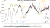 |
Fig. 1 Comparison of transit spectra including increased hydrocarbon abundances, with respect to a base of equilibrium chemistry abundances for the main molecular species with the hydrocarbons removed. The spectra shown are for a planet modelled onKepler-30c, with an equilibrium temperature of 769 K. |
NIRCam
The Near Infrared Camera (NIRCam) operates in the wavelength range of 0.6–5.0 microns, and offers various modes of operation4. The most relevant of these is the Grism Time Series mode, which has a resolving power of 1600 at 4 microns, and is able to observe the 2.4–5.0 micron range. Different parts of this wavelength range can be observed using different grisms, where F322W2 and F444W are included in PandExo (Batalha et al. 2017), the JWST instrument simulation package used in this work. F322W2 covers approximately 2.4– 4.2 microns, whereas F444W covers around 3.8 to 5.1 microns.
NIRISS
The Near Infrared Imager and Slitless Spectrograph (NIRISS) offers the possibility to observe the 0.6– 5.0 micron range, where the most relevant mode, single object slitless spectroscopy (SOSS), covers 0.6 to 2.8 microns5. There are various options for subarray use, and the resolving power is 700 at 1.4 microns.
2.2 Molecular data
The bulk of the analysis uses molecular data from the ExoMol database, with theoretical line lists largely designed to be suitable up to high temperatures (Tennyson et al. 2020). These line lists were formatted into opacities by Chubb et al. (2021) as part of the ExoMolOP database6. These theoretical determinations typically become increasingly computationally demanding as molecules gain more atoms and electrons. The molecules included in this database are thus limited, and the only hydrocarbons currently available are CH4 (Yurchenko et al. 2017), C2H2 (Chubb et al. 2020), and C2H4 (Mant et al. 2018). Other hydrocarbons, namely C2H6 and C4H2, are included as part of HITRAN (Gordon et al. 2017), a database of largely experimental data that has been measured at room temperature. For this reason, although HITRAN data is often very accurate (more accurate than purely theoretically calculated data), it is not considered complete as many of the weaker lines in particular are missing; it is only designed for temperatures in the region of 296 K or lower, with a few exceptions. In the Pacific Northwest National Laboratory (PNNL) experimental database, cross sections for C3H8 are also available, but this is again only valid for room temperature environments (Sharpe et al. 2002). Molecular spectra can change drastically for higher temperatures, making the experimental data invalid at the high-temperature environments mainly considered in this paper, due to hotter planets generally being better characterised than colder smaller planets. An example of this temperature variation for C2H2 can be found in Fig. 2, which shows the flattening of the spectra at higher temperatures. The line lists used in this study for CH4 and C2H2 are complete up to 2000 and 2200 K, respectively. The line list for C2H4 is only complete up to 700 K, and so we expect some opacity to be missing at higher temperatures, namely for the atmospheres of HD 189733b and HD 209458b. Therefore, we could be underestimating the detectability of C2H4 in these cases. It also has a lower wavelength cutoff of 1.4 μm, due to computational demands for computing higher-energy–lower-wavelength transitions. This means that the region covered by the NIRISS SOSS and NIRISS Prism is partly not covered by the opacity of C2H4. Nevertheless, the ExoMol MaYTY line list (Mant et al. 2018) is the most complete line list currently available for the main isotopologue of C2H4. Accurate molecular absorption data suitable for characterising atmospheres up to high temperatures are likely to become available for other hydrocarbon species such as C4H2 and C2H6 in the near future (Tennyson et al. 2020; Rothman et al. 2010; Rey et al. 2016; Bernath 2020). It is known from room temperature laboratory spectra that prominent absorption features for these species are expected within the infrared wavelength region accessible with JWST (Gordon et al. 2017). In particular, C2H6 is expected to be present in the upper atmospheres of certain carbon-rich gas giant exoplanets and brown dwarfs (Bilger et al. 2013). We therefore only focus on CH4, C2H2, and C2H4 for the current work, but hope to be able to expand to these other heavier hydrocarbon species in the future.
Physical properties of the exoplanetary systems considered in this study.
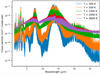 |
Fig. 2 Cross sections of C2H2 computed using the ExoMol aCeTY line list (Chubb et al. 2020) for a range of temperatures at a pressure of 0.1 bar. |
2.3 Planets considered in this study as the bases of our models
In the current study we focus on a small sample of planets that offer a range of physical properties based on the following: HD 189733b, HD 209458b, HD 97658b, and Kepler-30c. HD 189733b and HD 209458b are hot Jupiters orbiting bright stars, HD 97658b is a sub-Neptune orbiting a bright star, and Kepler-30c is a warm Jupiter orbiting a faint star. Table 2 gives some of the derived physical properties of the exoplanetary systems considered in this study. More details of the planets and previous detections are also given below. The model spectra we use in this study are from atmospheric models produced using the physical parameters of those planets listed here, but we do not use any observed data to produce them. Any clouds, for example, or atmospheric species that have potentially been detected (as detailed below) are thus not included. HD 189733b is an exception where we consider the effect of adding a cloud layer, as detailed in Sect. 3.2. We assume equilibrium chemistry based on the assumed equilibrium temperature of the planet for all species apart from the hydrocarbons of interest (C2H2, CH4, C2H4), which we add in at various abundances.
2.3.1 HD 189733b
HD 189733b is a hot Jupiter orbiting a K1-K2 type star approximately 19.3 parsec from Earth (Bouchy et al. 2005). The star’s flux in the near-infrared (J) band is 6.07 (Cutri et al. 2003). The emission spectra of HD 189733b will be observed using NIRCam’s slitless grism mode as part of the JWST Guaranteed Time Observations (GTO) programme (GTO 1274; P.I: Jonathan I. Lunine). In addition, a number of general observer (GO) programmes will observe HD 189733b in Cycle 1, including in transmission using NIRCam and MIRI MRS (GO 1633; P.I. Drake Deming) and MIRI LRS (GO 2001; P.I. Michiel Min), and an eclipse map also using MIRI LRS (GO 2021; P.I. Brian Kilpatrick). Evidence for CH4 in the transmission spectra of HD 189733b was first claimed to have been observed by Swain et al. (2008). CO and H2O have been detected on the dayside in high resolution (de Kok et al. 2013; Birkby et al. 2013), along with sodium (Wyttenbach et al. 2015) and potentially potassium (Keles et al. 2019) in the planet’s terminator region. H2O, CO, and HCN were all detected on the planet’s dayside at high resolution by Cabot et al. (2018).
2.3.2 HD 209458b
HD 209458b is a hot Jupiter orbiting a G0 V-type star approximately 47.0 parsec from Earth. The J-band flux of the star is 6.591 (Cutri et al. 2003), making its brightness when observed from Earth similar to that of HD 189733. As a consequence this planet is also very well studied. H2O was first claimed to be found by Barman (2007), and has been detected in the atmospheric transmission (Deming et al. 2013) and emission (Line et al. 2016) spectra of HD 209458b since then. CO and H2O, and potentially HCN, were detected in high resolution by Hawker et al. (2018). The presence of multiple molecules (H2O, CO, HCN, C2H2, CH4, and NH3) were recently detected in the atmosphere of HD 209458b by Giacobbe et al. (2021) using high-resolution spectra and cross-correlation methods. A high C/O for the planet’s atmosphere was inferred. Observations that indicate patchy clouds present at the terminator region of HD 209458b have been made by MacDonald & Madhusudhan (2017) and Barstow (2020). The emission spectra of HD 209458b will be observed using NIRCam’s slitless grism mode as part of the JWST Guaranteed Time Observations (GTO) programme (GTO 1274; P.I: Jonathan I. Lunine), and the transmission spectra with MIRI LRS as part of the GO programme (GO 2667; P.I: Hannah Wakeford).
2.3.3 HD 97658b
HD 97658b (Howard et al. 2011; Knutson et al. 2014) is much smaller than the hot Jupiters discussed previously, and is classified as a sub-Neptune or super-Earth. Its host star is of the K1V spectral type, and is approximately 21.1 parsec from Earth. Its J-band flux is 6.203 (Cutri et al. 2003). Not much is known about the atmosphere’s composition, although Guo et al. (2020) recently found that atmospheres with high C/O ratios (≥0.8) are favouredwhen compared to observed transmission data for HD 97658b. Guo et al. (2020) also found HD 97658b to be a high-priority target for atmospheric characterisation when assessing sub-Neptune exoplanets cooler than 1000 K. The planet’s relatively low temperature makes it a potentially good target for observing hydrocarbons using JWST.
2.3.4 Kepler-30c
Kepler-30c, despite being classified as a warm Jupiter, orbits a much fainter star than the targets mentioned previously, making it a more challenging object to observe. With a flux in the near-infrared of 14.00 magnitudes (Cutri et al. 2003), it is used to examine what instrument settings are best suited to observing faint targets. We note that this is an extremely faint target and that even instruments such as NIRSpec Prism have a J-band flux limit of 9.82 (Nielsen et al. 2016). It is thus included as an extreme case of a faint target, and we would expect better results from a similar but slightly brighter target. Not much is currently known about the planet’s atmosphere, most likely due to the host star being faint.
3 Methodology
3.1 Forward models using ARCiS
The ARtful modeling Code for exoplanet Science (ARCiS) package performs atmospheric modelling and Bayesian retrieval (see Min et al. 2020 and Ormel & Min 2019 for full details). The code consists of a forward modelling routine based on k-distribution molecular opacities from the ExoMolOP database (Chubb et al. 2021) and cloud opacities using Mie and distribution of hollow spheres (DHS; see Min et al. 2005) computations. With ARCiS one can compute cloud formation (Ormel & Min 2019) and chemistry (Woitke et al. 2018) from physical and chemical principles. The code was benchmarked against petitCODE (Molliére et al. 2015, 2017) by Ormel & Min (2019). For the retrieval part the MULTINEST algorithm (Feroz & Hobson 2008; Feroz et al. 2009, 2019) was employed to sample the specified parameter space for the region of maximum likelihood. Benchmarks for the retrieval were performed in the framework of the ARIEL mission (Pascale et al. 2018), showing excellent agreement with multiple other retrieval codes.
We first computed forward model atmospheres for each of our selected targets using ARCiS coupled with GGCHEM (Woitke et al. 2018) in order to obtain assumed equilibrium chemistry abundances of molecules and to compute the pressure-temperature structure of the atmosphere. These model atmospheres included the following molecules: H2O (Polyansky et al. 2018), CO2 (Yurchenko et al. 2020), CO (Li et al. 2015), CH4 (Yurchenko et al. 2017), NH3 (Coles et al. 2019), C2H2 (Chubb et al. 2020), TiO (McKemmish et al. 2019), and VO (McKemmish et al. 2016); the atmospheres were filled with H2 and He (at a ratio of 0.85:0.15, respectively). We included the most common constituents of atmospheres (H2O, CO2, CO, NH3), the three hydrocarbons considered in this study (CH4, C2H2, and C2H4), and two strong optical absorbers (TiO and VO). The temperature structure and molecular abundances were computed self-consistently using ARCiS (Min et al. 2020) coupled with GGCHEM (Woitke et al. 2018) for the equilibrium chemistry computations. Table 3 gives the molecular abundances and temperatures for the upper bound of the pressure layers (lower bound of altitude) that we would typically probe using transmission spectroscopy, as illustrated by Fig. A.1. These are the ‘base’ atmospheric compositions of each planet that we adopt, assuming an isothermal temperature structure and constant molecular abundances, which is not an unreasonable assumption when probing transmission spectra in this wavelength region (Zhang et al. 2019), although we note below this may lead to some potential biases. We subsequently added varying abundances of the hydrocarbons we are focusing on in this study (C2H2, CH4, C2H4) to the computed forward model atmospheres (at R =  = 300) using these base compositions. It can be seen from Fig. 3 that the difference between forward model spectra can be observed at a volume mixing ratio (VMR) of around 1 × 10⁻⁷–1 × 10⁻⁶. These example spectra are for a clear planet atmosphere with similar planetary and stellar properties to those of the HD 189733b system. As mentioned above, we computed our base models based on a layer of the atmosphere at approximately the upper limit of pressure that contributes to the observed transmission spectra for all planets. If we had chosen to model a lower-pressure layer, which has a greater contribution to the base spectra, there would be some effect on our initial model spectra. The main difference would be for the cooler planets, HD 97658b and Kepler-30c, where there is a greater variation in the temperature structure across the pressure layer that we expect to be probed by transmission spectroscopy, as can be seen in Figs. A.1 and A.2. Here we could be overestimating the temperature of our base models by a few hundred Kelvin. The main difference to the equilibrium chemistry would then be a lower CO abundance and higher CH4 abundance. Ideally, we would use a non-isothermal pressure-temperature parametrisation in our retrievals in order to limit any potential biases (Rocchetto et al. 2016; MacDonald et al. 2020).
3.2 Simulating JWST spectra using PandExo
Once the forward model spectra were computed with ARCiS, noise and other error sources were added to the spectrum inorder to simulate observations of our targets by various JWST instruments, as described in Sect. 2.1. This was done using PandExo, a Python package that is capable of simulating JWST measurements of transiting exoplanets (Batalha et al. 2017), and that can retrieve planetary and stellar properties from the online exoplanet database ExoMast7. Using this package, the data outputs of the instruments in various modes and using various subarrays can be simulated8. PandExo requires a noise floor and saturation limit that are instrument dependent. Both of these quantities are uncertain and will not be available until after the start of operation. However, the JWST User Guide gives approximate saturation limits for each instrument mode9 : 78% of full-well depth for MIRI; 70% of full-well depth for NIRCam time series and grism time series; 76% of full-well depth for NIRISS SOSS; 70% of full-well depth for NIRSpec’s full subarray; and 84% for the other subarrays. These values are used here. Furthermore, the noise floor level is even more unpredictable. Attempts have been made to approximate the noise floor levels by comparison with currently operational missions, resulting in 20ppm, 30ppm, and 50ppm for NIRISS (Kreidberg et al. 2014), NIRCam (Kreidberg et al. 2014), and MIRI (Knutson et al. 2009), respectively. Fortenbach & Dressing (2020) assume a noise floor level of25 ppm for NIRSpec. They argue that this is a conservative assumption, but it is in line with the noise floors of the other instruments and thus is used here. PandExo outputs a wide range of information, but the relevant parts for the observation file to be used for retrieval are the wavelengths, the output spectrum with random noise, and the error including the noise floor. The final part of the observation file is the spectral resolution per bin. We binned the data to a constant resolution of 100 in order to resize the data to a more manageable size for retrieval. PandExo also includes a binning tool, which was used for this purpose. The spectral resolution per bin is given by
 (1)
(1)
This observation file, with error bars added by PandExo, is then used for the free molecular retrievals (i.e. where we do not constrain molecular abundances based on equilibrium chemistry and allow them to vary freely) using ARCiS (Min et al. 2020; Ormel & Min 2019) (see Sect. 3.1). An illustration of the base equilibrium chemistry spectra for each of the four planets in this study is given in Fig. 4, along with the simulated spectra for the various JWST instruments used for each planet. We included both a clear and a cloudy model for HD 189733b. For the cloudy model we added in a fully opaque grey cloud layer at Ptop = 0.01 bar, and above that a Rayleigh scattering haze with a total opacity of fmix = 1 × 10² × H2. It can be seen that the cloudy model is similar to the clear model, but with muted molecular absorption features. The base spectrum of Kepler-30c is shown with and without the simulated JWST spectra, with the zoomed-in version included to make the main absorption features clearer.
Abundances of various species computed assuming equilibrium chemistry and solar C/O and metallicity using GGCHEM (Woitke et al. 2018) at ~1.8 × 10⁻¹ bar.
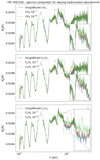 |
Fig. 3 Comparison of transmission spectra of a planet modelled on HD 189733b with varying hydrocarbon abundances. All species become visible at a VMR starting around 10−7. |
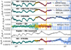 |
Fig. 4 Base spectra (computed from equilibrium chemistry) of each of the four planet types used in this study, as detailed in each panel. Both the clear and the cloudy models for HD 189733b are included. Simulated JWST spectra and the corresponding error bars using PandExo are also plotted for each instrument used in this study (see figure legend). |
3.3 Retrieval of JWST-simulated spectra using ARCiS
Using our simulated spectra for various JWST instruments (those highlighted in bold in Table 1 and illustrated in Fig. 4), we ran a series of retrievals on each spectrum. A summary of the set-ups for the models and retrievals of the four planets considered in this study can be found in Table 4, including the JWST instruments and modes used for each planet. These retrievals test how accurately we can retrieve what was input into the model atmospheres; see Sect. 3.4 for details on how this is quantified. In particular, we focus on whether the VMRs of the hydrocarbons of interest (C2H2, C2H4, and CH4) can be determined accurately. For this we allow free molecular retrievals with no conditions on the chemistry enforced. The free parameters and their ranges and priors are given in Table 5, and the planetary and stellar parameters used are given in Table 2. Although self-consistent temperature structures were computed for the forward models (see Fig. A.2), the retrieval assumes an isothermal atmosphere. This may result in an overestimation of the abundances and certainties for JWST’s capabilities (Rocchetto et al. 2016). We assumed a population size of 500 in the Multinest algorithm used for the retrievals.
3.4 Detection evidence from the Bayes factor
In order to determine the detectability of a particular hydrocarbon at a given VMR, we used the Nested Sampling Global Log-Evidence (log(E)) as a metric. This is given as an output from the Multinest algorithm (Feroz & Hobson 2008; Feroz et al. 2009, 2019). This Bayesian log-evidence is then used to find the Bayes factor (B01) (see e.g. Benneke & Seager 2013; Waldmann et al. 2015; Braam et al. 2021), which is a measure to assess the significance of one model against another and, given identical model priors, is reduced to the ratio of evidence (E). Here, ‘model’ refers to the set of free parameters included in the retrieval, in particular if we include the hydrocarbon of interest (whose VMR we are varying) or not. If the Bayes factor B01 > 5, then according to Trotta (2008) the model can be considered significant with respect to the ‘base’ model: B01 > 5 corresponds to >3.6 σ detection over the base model; B01 > 11 corresponds to >5 σ detection over the base model; B01 < 1 indicates that the evidence is not significant; 1 < B01 < 2.5 indicates weak evidence; 2.5 < B01 < 5 indicates moderate evidence; B01 > 5 indicates strong evidence; and B01 > 11 indicates very strong evidence.
Instrument and abundance set-ups for the models and retrievals of the four planets considered in this study.
Parameters and the corresponding ranges and priors used in the retrievals in this study.
4 Results
We attempted to quantify the minimum values of the VMR that are observable for each molecule, planet, and instrument (or instrument combination). In Tables 6–10 we specify the Bayes factor, B01, for each retrieval set-up, comparing the retrieval with the specified molecule (C2H2, C2H4, CH4) included versus not included. In all cases the specified molecule was included in the initial forward atmospheric simulation, at the log(VMR) specified. Based on Trotta (2008), we consider all cases with B01 ≥ 5 to be significant. More details are provided below for each planet, with notes on the differences between the detectability of the three species (C2H2, CH4, C2H4) for different instruments.
Bayes factor (B01) for various retrievals for HD 209458b.
Bayes factor (B01) for various retrievals for HD 189733b.
4.1 HD 189733b and HD 209458b
The posterior distributions of all hydrocarbon VMRs retrieved for various abundances (1 × 10⁻⁴ or 1 × 10⁻⁶ for CH4, C2H2, and C2H4) are collected in Figs. 5–10 for the single instrument set-ups of HD 189733b, HD 209458b, and HD 97658b. The posterior distributions for the VMRs of the other hydrocarbons are also given in each case. We give a short summary for each instrument or instrument combination for these two planets below.
4.1.1 HD 189733b and HD 209458b: MIRI LRS
MIRI LRS is able to detect the 5–12 micron range. The outcome is similar for both planets: all species are retrieved with high evidence when in an abundance of 10−4, but difficulties occur around the 10−6 mark. The Bayes factors in Tables 6 and 7 become <1 at this point. Interestingly, for the 10−6 cases, C2H2 is moderately detectable in both planets, while there is no significant evidence for C2H4 at all. Observations using MIRI LRS may be relatively noisy, especially at wavelengths longer than 10 μm. As shown in Figs. 1 and 3, the most distinct features for C2H4 occur in this range, while at the shorter wavelengths of MIRI’s range C2H2 and CH4 have overlapping features. Therefore, in lower abundances C2H4 may be overshadowed by noise, while features of CH4 could be attributed to C2H2 and vice versa. This is evident in the posterior distribution plot for C2H2 of Fig. 6 in the case of HD 189733b, where VMR(CH4) = 1 × 10⁻⁶ (and C2H2 should be in negligible abundance). Similarly, in the case of HD 209458b using MIRI LRS, Fig. 8 shows that a peak becomes visible in the posterior distribution of CH4 at a higher abundance than it should be, for the case where VMR(C2H2) = 1 × 10⁻⁶.
4.1.2 HD 189733b and HD 209458b: NIRISS SOSS
NIRISS SOSS operates in the 0.6 to 2.8 micron range, where, as shown in Fig. 1, the strongest signatures are from CH4 and C2H4. C2H2 also shows signatures here, but they are not significant and could easily be overshadowed by the other hydrocarbons when these are sufficiently abundant. Similarly to MIRI LRS, detection becomes more uncertain for an abundance of 1 × 10⁻⁶. Contrary to MIRI LRS, however, all Bayes factors are <1 in these cases. The cause for this is likely of the same nature; Fig. 1 demonstrates that CH4 and C2H4 overlap in its wavelength range, while the features of C2H2 are narrow and weak. The corresponding posterior of C2H4 in Fig. 6 (for HD 209458b where VMR(CH4) = 10−6) shows that C2H4 is retrieved as abundant when it should be negligible. Figure 10 (where VMR(C2H4) = 10−6) shows a higher retrieved abundance for CH4 than it should, in particular for HD 209458b. These cases indicate that removing the species of interest can still result in a good fit with the other hydrocarbon present in a higher VMR, which leads to a low value of B01. We therefore find that for lower abundances NIRISS SOSS is likely capable of finding that a hydrocarbon is present, but seems unable to ascertain which one.
Bayes factor (B01) for various retrievals for HD 189733b, which include a cloud deck at Ptop = 0.01 bar with a scattering slope of fmix = 1 × 10² × H2 scattering.
Bayes factor (B01) for various retrievals for HD 97658b.
4.1.3 HD 189733b and HD 209458b: NIRCam F322W2
The detectable wavelength range of NIRCam F322W spans approximately 2.4 to 4.2 microns, where the hydrocarbon signatures are strong and unique. The Bayes factors (Tables 6 and 7 for HD 209458b and HD 189733b, respectively) are larger than 5, and in many cases larger than 11, for all three hydrocarbons, even for VMRs of 10−6. The equilibrium abundance of CH4 in HD 189733b is sufficient to be detectable in the absence or lower abundance of other species, evidenced by the distributions in Fig. 8 for VMR(C2H2) = 10−6 and in Fig. 10 for VMR(C2H4) = 10−6, but 1 × 10⁻⁷ is not. NIRCam F322W2 has very fewproblems distinguishing between the hydrocarbons, as opposed to NIRISS SOSS. The only notable example is the inability to find CH4 when C2H2 is increased to 10−4 in HD 189733b (see Fig. 7). Although NIRCam F322W2 is still able to strongly detect CH4 at a VMR of 10−6 for the cloudy atmosphere case for HD 189733b, only moderate detections are found for C2H2 or C2H4 at the same VMR (see Table 8).
Bayes factor (B01) for various retrievals for Kepler-30c.
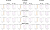 |
Fig. 5 Posterior distributions from retrievals of model atmospheres of HD 189733b, HD 209458b, and HD 97658b for an input CH4 abundance of 10−4 (orange) andC2H2 and C2H4 in their respective equilibrium abundances (purple). The results using a variety of instruments are given. The model input abundance is indicated by a black line, which is not shown when lower than the presented range. |
4.1.4 HD 189733b and HD 209458b: NIRSpec G395M
Tables 6 and 7 (for HD 209458b and HD 189733b, respectively) demonstrate that the performance of NIRSpec G395M is very similar to NIRCam F322W2, with both set-ups operating in approximately the same wavelength range. Even when clouds are included in our model atmospheres and retrievals, NIRSpec G395M gives strong evidence for the presence of all hydrocarbons down to a VMR of 10−6 (see the Bayes factors in Table 8). This is an improvement in comparison to using NIRCam F322W2 for the cloudy HD 189733b atmospheres. NIRSpec, just like NIRCam, is able to detect the equilibrium abundance of CH4 in HD 189733b for the cases where VMR(C2H4) and VMR(C2H2) are 10−6, but starts to have issues when these are increased to 10−4, particularly for VMR(C2H4) = 10−4 (Fig. 9). There are a few more cases where hydrocarbons interfere with one another, namely for VMR(CH4) = 10−6 in HD 209458b (Fig. 6), where C2H2 is retrieved when it should be at negligible abundance, but also VMR(C2H4) = 10−6 (Fig. 10) where C2H2 is similarly retrieved when it should not be.
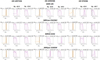 |
Fig. 6 Posterior distributions from retrievals of model atmospheres of HD 189733b, HD 209458b, and HD 97658b for an input CH4 abundance of 10−6 (orange) andC2H2 and C2H4 in their respective equilibrium abundances (purple). The results using a variety of instruments are given. The model input abundance is indicated by a black line, which is not shown when lower than the presented range. |
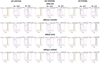 |
Fig. 7 Posterior distributions from retrievals of model atmospheres of HD 189733b, HD 209458b, and HD 97658b for an input C2H2 abundance of 10−4 (orange) andC2H4 and CH4 in their respective equilibrium abundances (purple). The results using a variety of instruments are given. The model input abundance is indicated by a black line, which is not shown when lower than the presented range. |
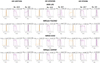 |
Fig. 8 Posterior distributions from retrievals of model atmospheres of HD 189733b, HD 209458b, and HD 97658b for an input C2H2 abundance of 10−6 (orange) andC2H4 and CH4 in their respective equilibrium abundances (purple). The results using a variety of instruments are given. The model input abundance is indicated by a black line, which is not shown when lower than the presented range. |
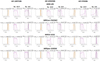 |
Fig. 9 Posterior distributions from retrievals of model atmospheres of HD 189733b, HD 209458b, and HD 97658b for an input C2H4 abundance of 10−4 (orange) andC2H2 and CH4 in their respective equilibrium abundances (purple). The results using a variety of instruments are given. The model input abundance is indicated by a black line, which is not shown when lower than the presented range. |
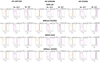 |
Fig. 10 Posterior distributions from retrievals of model atmospheres of HD 189733b, HD 209458b, and HD 97658b for an input C2H4 abundance of 10−6 (orange) andC2H2 and CH4 in their respective equilibrium abundances (purple). The results using a variety of instruments are given. The model input abundance is indicated by a black line, which is not shown when lower than the presented range. |
4.1.5 HD 189733b and HD 209458b: NIRISS SOSS and NIRSpec G395M
Batalha & Line (2017) find that increasing the wavelength range is more effective than using the same instrument twice, as is done when observing multiple transits. We therefore test various instrument combinations. Furthermore, they find that the combination of NIRISS SOSS and NIRSpec G395M yields the most information and the best results. We present a selection of the results for the combined instrument retrievals in Fig. 11. Combining these two instrument modes shows improvements for retrieving the abundances of C2H2 and C2H4 in HD 209458b in terms of the Bayes factors (Table 6). No improvements are observed for HD 189733b when compared to using NIRSpec G395M by itself, as NIRSpec G395M alone was already very accurate for HD 189733b. While the evidence for the other two hydrocarbons has improved, the strange shape of the C2H2 distribution remains for CH4 increased to 10−6 in HD 209458b in Fig. 11. Although this instrument combination appears to offer an accurate retrieval for abundances down to 10−6, we note that the improvements are not drastic in comparison to using NIRSpec G395M alone. This is likely due to the performance of NIRISS SOSS alone, which does not cover a beneficial wavelength region for the detection of the hydrocarbons we are interested in.
4.1.6 HD 189733b and HD 209458b: NIRSpec G395M and MIRI LRS
The combination of NIRSpec G395M and MIRI LRS covers a wide range of wavelengths, including the longer wavelengths expected to be minimally affected by hazes blocking the spectrum. In such cases, using a different combinationof instruments could yield more information regarding molecular abundances than the combination treated previously of NIRISS SOSS and NIRSpec G395M, which operates in the shorter wavelengths. We set out to test whether there is an advantage to using this instrument combination as opposed to one of the single instruments alone. In particular, there were previous issues in accurately determining the VMR of C2H2 in HD 189733b down to low values for these instruments individually. Similarly to the combination discussed above, we find an improvement in evidence for C2H2 and C2H4 in HD 209458b in comparison to using either instrument alone (Table 6). For HD 189733b, the performance is just as goodas NIRSpec G395M individually but there is improvement in comparison to using MIRI LRS alone (Table 7). We find, however, that combining these instruments does not reduce the retrieved abundance of C2H2 in HD 209458b in the case where VMR(CH4) = 10−6, which should be negligible (Fig. 11).
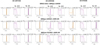 |
Fig. 11 Posterior distributions from retrievals using selected combinations of instruments of model atmospheres of HD 189733b, HD 209458b, and HD 97658b for an input abundance of 10−4 for the main hydrocarbon specified (orange) and other species in their respective equilibrium abundances (purple). The model inputabundance is indicated by a black line, which is not shown when lower than the presented range. |
4.1.7 HD 189733b and HD 209458b: NIRCam F322W2 and MIRI LRS
This combination of instruments demonstrated an improvement in comparison to the individual instruments alone. Although NIRCam F322W2 alone offered medium to strong detections in all cases, this was improved to very strong detections in all cases when combined with MIRI LRS. This can be seen in the Bayes factors of Table 6 (for HD 209458b) and Table 7 (for HD 189733b). An illustration of the different spectra retrieved using this instrument combination, with and without each of the molecules (CH4, C2H2, C2H4) included in the retrieval, is given in the right panels of Figs. A.3 and A.4. Here the retrieval with the molecule included (best-fit spectra in purple) fits the observed data points better than the retrieval with the molecule removed (best-fit spectra in orange) for HD 189733b. Similar figures for HD 209458b can be found in the supplementary information document10 associated with this work. Additionally, the false detection of C2H2 in HD 209458b that occurs in the NIRSpec results does not occur here, or for NIRCam F322W2 alone. This can be seen in Fig. 6, where VMR(CH4) = 10−6.
4.1.8 HD 189733b: Clouds
The presence of clouds and hazes can cause flattening of the spectrum, as can be seen for HD 189733b in Fig. 4. They also cause a scattering slope, which largely affects spectra at shorter wavelengths than we consider in this study. These muted features may complicate the detection of molecular species in atmospheres. As such, we have included a case of HD 189733b with a cloud layer at Ptop = 0.01 bar, and a scattering slope with fmix = 1× 10² × H2 scattering. The corresponding Bayes factors are included in Table 8. Overall, the inclusion of clouds in this configuration does not seem to significantly reduce the evidence of the hydrocarbon detections; we mainly see a reduction in the results for MIRI LRS and NIRCam F322W2. In addition to the deterioration in evidence, both NIRCam F322W2 and its combination with MIRI LRS are now unable to confidently find CH4 in equilibrium abundance when VMR(C2H2) = 10−6 (see Fig. 12), while this was previously possible (Figs. 8 and 11). On the other hand, this problem does not occur for NIRCam F322W2 when VMR(C2H4) = 10−6 (also shown in Fig. 12). The NIRSpec G395M observations are not affected by this, as shown in the bottom right set of the same plots. The full posterior plots, illustrating the clear versus cloudy case for HD 189733b for various instruments and combinations of instruments, can be found in the supplementary information document associated with this work, along with selected retrieved spectra for the cloudy case.
4.1.9 HD 189733b and HD 209458b: Summary
The most accurate results were found using the combinations of either NIRCam F322W2 and MIRI LRS or NIRSpec G395M and MIRI LRS. Although the results from NIRCam F322W2 and NIRSpec G395M were similar, it seems particularly beneficial to use NIRSpec G395M over NIRCam F322W2 in the case of a cloudy atmosphere for HD 189733b. In addition, we note that improvements in the retrieved abundances of other non-hydrocarbon species (although not detailed here) are also generally found by extending the wavelength region observed. We include some posterior distributions including the full range of molecules in the supplementary information to this work. The input model abundances are given as red vertical lines in all plots. In general we note a few observations. Firstly, the combination of NIRISS SOSS and NIRSpec G395M, although not found to be optimal for detecting the hydrocarbon molecules we are interested in, gives reasonable and well-constrained abundances for TiO, VO, CO2, and CO (for both HD 189733b and HD 209458b). In general, H2O is retrieved reasonably for all instrument combinations, although in some cases it is found to be slightly more abundant than in the input models. It can also be observed for both planets that the abundances of CO and CO2 are retrieved confidently around the input values for NIRSpec G395M and MIRI LRS, but not for NIRCam F322W2 and MIRI LRS. We note, however, that in the case of HD 209458b that C2H2 is often retrieved in the cases where it should not be for NIRSpec G395M and MIRI LRS, but this issue does not occur for NIRCam F322W2 and MIRI LRS. Even so, we conclude that generally the best choice for observing HD 189733b and HD 209458b is probably NIRSpec G395M and MIRI LRS (combined), particularly if clouds are expected, based on the results of HD 189733b, with NIRCam F322W2 and MIRI LRS (combined) a close second.
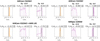 |
Fig. 12 Retrieval results using NIRCam F322W2 and its combination, and NIRSpec G395M for HD 189733b when including clouds and a scattering slope, for increased C2H2 and C2H4 abundance to 10−6 (orange), respectively. The remaining species are in equilibrium abundance (purple) in each set of columns. The modelinput abundance is indicated by a black line, which is not shown when lower than the presented range. |
4.2 HD 97658b
The posteriors of all hydrocarbons retrieved for various abundances (of 1 × 10⁻⁴ or 1 × 10⁻⁶ for CH4, C2H2, and C2H4) are collected in Figs. 5–10 for the single instrument set-ups of HD 189733b, HD 209458b, and HD 97658b (with HD 97658b in the right-hand columns). The Bayes factors for HD 97658b can be found in Table 9.
4.2.1 HD 97658b: MIRI LRS
The smaller transit depth and larger relative error (see Fig. 4) in the observed spectra of HD 97658b makes it more difficulte to differentiate between hydrocarbon signatures. As such, no certain detections occur for VMRs of 10−6, which results in Bayes factors of <1 for all cases in Table 9. When in lower abundance, the features can be attributed to different hydrocarbons, resulting in a good fit whether the species of interest is included or not. The equilibrium abundance of CH4 is significant enough that it should be able to be detected (see Table 2), but in Fig. 7 (VMR(C2H2) = 10−4) and Fig. 9 (VMR(C2H4) = 10−4) it can be seen that it is not confidently retrieved when the other hydrocarbons are of significant abundances. The posteriors are more constrained for CH4 in Figs. 8 and 10, where VMR(C2H2) = 10−6 and VMR(C2H4) = 10−6, respectively.
4.2.2 HD 97658b: NIRISS SOSS
Similar to the results for MIRI LRS, NIRISS SOSS is unable to retrieve when the abundance is 10−6 and lower. However, the high equilibrium abundance of CH4 is found here in combination with the other hydrocarbons even when they are significant (VMR of 10−4, see Fig. 7 for C2H4 and Fig. 9 for C2H2).
4.2.3 HD 97658b: NIRCam F322W2
NIRCam F322W2 performs better than both MIRI LRS and NIRISS SOSS for HD 97658b, as was the case for HD 189733b and HD 209458b. It is able to accurately retrieve CH4 down to an abundance of 10−6, without influencing the distribution of C2H2 abundances (see Fig. 6). The posterior plot in Fig. 8 starts to become skewed for C2H2, and the Bayes factor indicates that there is no statistical evidence that C2H2 can be retrieved at this abundance using NIRCam F322W2 alone. The retrieved CH4 abundance is reasonable but slightly higher than it should be when the VMR of C2H2 is 10−6, possibly due to difficulties in differentiating between these hydrocarbon species. C2H4 is not retrievable at an abundance of 10−6 (see Fig. 10), probably due to the high equilibrium CH4 abundance, which again in this case is retrieved reasonably well, but slightly higher than in the input models. Additionally, we note that the distributions in Fig. 5 (where VMR(CH4) = 10−4) look peculiar, with some likelihood of a C2H4 contributionbeing found. Overall, NIRCam F322W2 does not seem to be able to distinguish between the different hydrocarbons as well as it did for HD 189733b and HD 209458b. We therefore test cases where the number of transits is increased to 25 (see Sect. 4.2.8), as well as the instrument combinations considered previously.
4.2.4 HD 97658b: NIRSpec G395M
The performance of NIRSpec G395M is again very similar to NIRCam F322W2, where C2H4 or C2H2 for abundances of 10−6 are not detected, see Table 9 and the corresponding posterior plots in Figs. 5 to 10.
4.2.5 HD 97658b: NIRISS SOSS and NIRSpec G395M
We note that especially C2H4 in a VMR of 10−6 in combination with the equilibrium abundance of CH4 proved difficult to find using all single instruments tested. In an attempt to resolve these issues, we examine the same instrument combinations as for HD 189733b and HD 209458b, the resulting posterior distributions of which can be found in Fig. 11. The Bayes factors for all other cases are again presented in Table 9. Combining these two instrument modes shows great improvements in comparison to the individual instruments for most cases in HD 97658b, resulting in very confident retrievals for all cases apart from when VMR(C2H2) = 10−6. The Bayes factor corresponding to C2H4 with a VMR of 10−6 is in excess of 11, indicating that it is now retrieved. Interestingly, the distribution is not a single narrow peak in this case, which indicates that the exact abundance is not as certain as appears based on the Bayes factor alone.
4.2.6 HD 97658b: NIRSpec G395M and MIRI LRS
We find the improvements when combining NIRSpec G395M and MIRI LRS to be minor in comparison to NIRSpec G395M alone when examining the Bayes factors of Table 9. The retrieved abundances based on Fig. 11 now seem to be well constrained.
4.2.7 HD 97658b: NIRCam F322W2 and MIRI LRS
There were some issues with these individual instruments; both were unable to retrieve C2H4 or C2H2 at a VMR of 10−6 (see the Bayes factors in Table 9), and MIRI LRS could also not retrieve CH4 at a VMR of 10−6. Both MIRI LRS and NIRCam F322W2 had some trouble distinguishing between different hydrocarbon species. Combining the instruments shows a great improvement for all these issues, and is found to be far more accurate than using the single instruments alone (see, for example, the posterior distributions in Fig. 11). The factors in Table 9 indicate this to be the best instrument combination to use for our selected small target.
4.2.8 HD 97658b: Multiple transits
Batalha et al. (2015) find that observing multiple transits shows advantages for smaller targets like super-Earths and other small objects. As such, this set-up is tested for HD 97658b. Based on the Bayes factors in Table 9 and the results of selected species in Fig. 13, we find in general that there are improvements in some cases of retrievals when the number of transits is increased to 25 in comparison to a single transit, as demonstrated by the increase in B01 in Table 9 for smaller abundances. However, the increase in observational time likely does not justify these small improvements, and we found similar or even better improvements when different instruments were combined to give a larger wavelength coverage. While the multiple transits only improve the detection limit of C2H2 to 10−6, a significant increase in B01 is found for C2H4 abundances of 10−6 as well using the instrument combination NIRCam F322W2 and MIRI LRS.
4.2.9 HD 97658b: Summary
The most accurate instrument combination for HD 97658b was found to be NIRCam F322W2 and MIRI LRS (combined). The improvements compared to the individual instruments alone was found to be much greater in the case of this planet than with the more favourable targets of HD 189733b and HD 209458b. Similar observations for HD 189733b and HD 209458b can be made for HD 97658b regarding the posterior distributions of the other (non-hydrocarbons) molecules included in the input models, which can be found in the supplementary information document of this work. H2O is retrieved reasonably well for all of the following instrument combinations. CO and CO2 are are retrieved reasonably well for NIRSpec G395M and MIRI LRS (although the abundances are slightly too high in some cases), but not for NIRCam F322W2 and MIRI LRS. NIRISS SOSS and NIRSpec G395M generally gives confident and reasonably accurate retrievals of the abundances of CO, CO2, VO, and TiO in comparison to their input values, which are given as red lines in all figures. While observing multiple transits does improve the detection limits and certainty, a significantly longer observational time may be required. We therefore find that a single transit using the combination of NIRCam F322W2 and MIRI LRS is preferable to using 25 transits for any individual instrument for HD 97658b.
4.3 Kepler-30c
4.3.1 Kepler-30c: Standard instrument set-ups
The Bayes factors and posterior plots for our selected faint target can be found in Table 10 and Figs. 14and 15. The standard instrument set-ups, which refer to MIRI LRS, NIRISS SOSS, NIRCam F322W2, and NIRSpec G395M, perform quite poorly overall for Kepler-30c. MIRI LRS, NIRISS SOSS, NIRSpec G395M, and NIRCam F322W2 are all unable to find any hydrocarbons, based on the Bayes factors of Table 10. Of these standard single instrument set-ups, NIRSpec G395M looks the most reasonable based on the posterior distribution for the case where VMR(CH4) = 10−4, as shown in Fig. 14. Both the slitless mode, which is the most commonly used in this study, and the slit mode were tested for MIRI LRS. This was done since using the slit could have advantages for faint objects due to a reduction in background light, but our results confirm the findings of Howe et al. (2017), since no improvements were found when using the slit mode as a single instrument.
4.3.2 Kepler-30c: NIRSpec Prism
Batalha & Line (2017) suggest using NIRSpec Prism for detecting faint objects. The mode is easily saturated, but may be better for observing objects like Kepler-30c. NIRSpec Prism covers a relatively wide range of wavelengths, approximately from 0.6 to 5.3 μm; the resolving power is comparable to MIRI LRS (~100 nominally). We found that NIRSpec Prism shows weak detection (>1 in Table 10) of CH4 down to the VMR = 10−4 region, but is unable to find hydrocarbons at VMR = 10−6. Furthermore, the equilibrium abundance of CH4 is VMR = 10−3.16, which possibly inhibits detection of the other hydrocarbons. In fact, CH4 is consistently retrieved at an abundance higher than the input abundance, most likely due to C2H2 or C2H4 being present and increasing the strength of the features (see the narrowly constrained distributions in Fig. 15). Even for the case where VMR(CH4) = 10−4, the abundance retrieved is too high, as shown in Fig. 14. In the presence of abundant CH4 it becomes incredibly difficult to find less abundant hydrocarbons in faint objects like Kepler-30c.
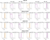 |
Fig. 13 Posterior distributions from retrievals using 25 transits of model atmospheres of HD 97658b, for increased CH4 and C2H4 abundances of 10−6 (orange) and equilibrium abundance of the remaining species (purple). The model input abundance is indicated by a black line, which is not shown when lower than the presented range. |
4.3.3 Kepler-30c: NIRSpec Prism and MIRI LRS
The combination NIRSpec Prism and MIRI LRS covers the widest wavelength range achievable with the instrument settings currently included in PandExo: 0.6–12 microns. Again, here we test both the slit and slitless modes of MIRI LRS. The performance including the slitless mode is approximately the same as using NIRSpec Prism by itself (see Table 10), and thus there are no advantages that would warrant using this instrument combination for faint objects like Kepler-30c. However, minor improvements are found when combining NIRSpec Prism with MIRI LRS slit (see Fig. 15 and Table 10).
4.3.4 Kepler-30c: Summary
In summary, Kepler-30c is not an easy target to accurately detect signatures of the hydrocarbons we are looking for using the instruments tested here. We note that the stellar brightness of Kepler-30 is below that recommended for all instruments tested, even NIRSpec Prism which is designed for fainter targets. In addition, due to the low equilibrium temperature of Kepler-30c, the equilibrium chemistry simulations yield quite a high CH4 abundance, which can make distinguishing between different hydrocarbons more challenging. In the presence of abundant CH4 it becomes incredibly difficult to find less abundant hydrocarbons in faint objects like Kepler-30c. We find limited benefits of combining NIRSpec Prism with MIRI LRS observations over observing with NIRSpec Prism alone. We find worse results when using NIRSpec G395M in comparison to observing with NIRSpec Prism, but find that there is some slight improvement when combining NIRISS SOSS and NIRSpec G395M in comparison to NIRSpec G395M alone. Based on the posterior plots alone (see Figs. 14 and 15), NIRISS SOSS and NIRSpec G395M appear to be better for retrieving C2H4 at a VMR of 10−4. This is not mirrored by the Bayes factors in Table 10, although we note that the difference between the two is not significant. The posteriors for NIRISS SOSS and NIRSpec G395M (combined) and NIRSpec Prism are similar for retrieving CH4 at a VMR of 10−4. NIRSpec Prism is probably the best choice in terms of performance and to avoid using more than one instrument unnecessarily or to observe multiple transits, although there is a very minor improvement when MIRI LRS slit is combined with NIRSpec Prism. Our findings support the guidance that the JWST instruments are not suited to targets with a J-band flux fainter than 9.82 (Nielsen et al. 2016), but they hint that a slightly brighter but still faint target could benefit from the use of NIRSpec Prism and MIRI LRS slit (combined), or potentially NIRISS SOSS and NIRSpec G395M (combined).
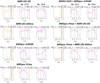 |
Fig. 14 Posterior distributions from retrievals using a variety of instruments for Kepler-30c, for increased CH4 abundance to 10−4 (orange) and equilibrium abundance for the remaining species (purple) in each set of columns. The model input abundance is indicated by a black line, which is not shown when lower than the presented range. |
4.4 Distinguishing absorption features
As discussed previously, it can sometimes be difficult to distinguish between different hydrocarbons, since some signatures are in similar wavelength regions. It was found that a large abundance of one hydrocarbon, here most often methane, results in other hydrocarbons not being detected or in large uncertainties in detection. This could be caused by random noise pushing the best fit to the wrong model spectrum or being somewhere in between. For example, NIRCam F322W2 and NIRSpec G396M observe partially overlapping parts of the spectrum, yet NIRSpec G395M incorrectly finds C2H2 in HD 209458b when CH4 is increased to a VMR of 10−6 (see Fig. 6), while NIRCam F322W2 does not. When examining the observations around the range of a prominent C2H2 feature (see Fig. 1) in Fig. 16, we see that the simulated spectra using NIRSpec G395M shows a deeper transit depth (i.e. more absorption) than the same region from NIRCam F322W2, therefore causing the retrievals using the NIRSpec G395M simulated spectra to find C2H2 where it should be insignificant. However, some wavelength ranges seem better suited to distinguishing between different hydrocarbons than others, due to the difference in nature of signatures between wavelength ranges. Both NIRSpec G395M and NIRCam F322W2 are best at differentiating between the hydrocarbons since they operate in asimilar wavelength range where wider and more unique signatures can be found. MIRI LRS is not able to distinguish between the hydrocarbons as well as NIRSpec G395M and NIRCam F322W2, but performs slightly better than NIRISS SOSS, which performed worst. This is most likely due to the widest and most unique signatures being present in the mid-IR range. A large part of this is covered by MIRI LRS, but the majority of the major C2H2 signatures are at the end of the wavelength range where the error of MIRI LRS increases significantly. The larger error causes smaller changes, for example in the 10−6 range, to be harder to detect. Furthermore, the noise floor of MIRI is the highest of all instruments, preventing it from reaching the same precision as NIRSpec G395M and NIRCam F322W2. We therefore find optimum results when different instruments are combined. In particular: NIRSpec G395M–MIRI LRS and NIRCam F322W2–MIRI LRS. We note that the presence of hydrocarbon hazes (see Sect. 5.2) may mute absorption features in the shorter wavelength regions in particular, so instrument combinations that include MIRI LRS may be preferable.
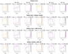 |
Fig. 15 Posterior distributions from retrievals using a variety of instruments and instrument combinations for Kepler-30c, for increased hydrocarbon abundances to 10−4 (orange) and equilibrium abundance for the remaining species (purple) in each set of columns. The model input abundance is indicated by a black line, which is not shown when lower than the presented range. |
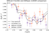 |
Fig. 16 Comparison of the observations for NIRCam F322W2 and NIRSpec G395M, for HD 209458b with CH4 increased to 10−6 (true spectrum), and C2H2 increased to 3⋅10−7 (as found from NIRSpec G395M observations). |
5 Discussion
5.1 Different chemistry models
The importance of including hydrocarbons in chemical reaction schemes is discussed by Venot et al. (2015), who show that these extra reactions are especially relevant for cooler atmospheres with T < 1000 K and for hotter atmospheres when C/O > 1. A similar conclusion is reached by other works such as Madhusudhan (2012), who perform a study on the effects of different C/O ratios on the atmospheric composition of hot Jupiters when assuming equilibrium chemistry. The assumption of chemical equilibrium is generally thought to hold for hot planets since this class of planets is less affected by disequilibrium effects than those with Teq < 1200 K. Madhusudhan (2012) find that for C/O > 1 a change in properties occurs for Teq > 1200 K, where the atmosphere may contain abundant C2H2 and HCN in addition to CH4, although CO remains the dominant carbon bearing species. Molliére et al. (2015) use a similar assumption in their model, where planets with Teff ≥ 1500 K are assumed to be unaffected by disequilibrium processes, based on the findings of Miguel & Kaltenegger (2014). Theoretical models such as these thus predict that it is difficult to find hydrocarbons at detectable abundances when considering equilibrium chemistry alone, unless C/O is very high. In this case a combination of very high temperatures and high C/O (at least higher than unity) can result in highly abundant hydrocarbons, where heavier hydrocarbons can surpass CH4 in abundance. This is mainly applicable to C2H2, which is not destroyed by high temperatures like C2H4.
On the other hand, planets with an effective temperature of around 1500 K or less are expected to have atmospheres strongly affected by disequilibrium processes such as vertical mixing (Miguel & Kaltenegger 2014; Tsai et al. 2017). Vertical mixing essentially allows us to probe a deeper layer of the atmosphere than we would otherwise be able to see, and tends to enhance the abundances of species such as CH4, C2H2, and C2H4 for all C/O ratios, but particularly for C/O 1 (Moses et al. 2012; Bilger et al. 2013; Tsai et al. 2017). Methane and acetylene have been found to be amongst the most instructive species when it comes to diagnosing vertical mixing effects in an exoplanet’s atmosphere (Tsai et al. 2017). Accurate abundance measurements of these species thus allow for evidence to be inferred not only of C/O, but also of atmospheric vertical mixing strength (quantified by the eddy diffusion coefficient, Kzz). Photodissociation is also thought to play a key role in producing higher abundances of hydrocarbons (Venot et al. 2015). Detection of hydrocarbon species other than methane will therefore provide important information on both disequilibrium chemistry processes and C/O ratio.
5.2 Effect of hydrocarbon hazes on detectability
It is expected that haze formation will become efficient at temperatures below around 1000 K (Kawashima & Ikoma 2019), and so we would expect it to particularly affect the atmospheres, and therefore transmission spectra, of Kepler-30c and HD 97658b out of the planets considered in this study. There are many uncertainties related to haze formation, and the models discussed previously rely on many assumptions regarding haze precursor types and particle size and shape, but also the fraction of haze precursors that in the end form a haze and mixing effects. Since these factors can affect the haze thickness, the resulting spectra can differ greatly depending on the assumptions. As such, it is essential to gain more information about the processes involved. The detection of the haze and molecules present in deeper layers of the atmosphere can be of use here. However, the haze can block large parts of the spectrum. Overall, lower C/O ratios and irradiation intensities combined with higher equilibrium temperatures result in clearer atmospheres (see e.g. Figs. 9 and 12 in Kawashima & Ikoma 2019), which are favourable when identifying the atmosphere’s composition. However, these conditions are exactly the opposite of what is required for complex hydrocarbon formation. As such, it is expected that atmospheres with abundant complex hydrocarbons could be greatly affected by hazes, thus making their identification more difficult. NIRISS SOSS will be most affected by hazes because its wavelength range is in the shorter wavelengths close to where a spectral slope occurs. Longer wavelengths, specifically in the MIRI region, will generally be less affected by haze effects, making it an interesting option for detecting molecular abundances. However, very thick hazes can result in flattening over the entire spectrum where wider wavelength ranges are better suited (see e.g. Greene et al. 2016), likely making instrument combinations a better option.
6 Conclusion
In this work we have investigated the detectability of some major hydrocarbon species (C2H2, CH4, and C2H4) in various types of exoplanets: two favourable hot Jupiter targets modelled on HD 189733b and HD 209458b; a smaller super-Earth/sub-Neptune modelled on HD 97658b; and a warm Jupiter orbiting a faint star modelled on Kepler-30c. We simulated the expected observed transit spectra of these planets using various instruments on board the JWST, using the PandExo package (Batalha et al. 2017). We used the retrieval package ARCiS (Min et al. 2020; Ormel & Min 2019) with opacities from the ExoMolOP database (Chubb et al. 2021) to run a retrieval and compared the results to the model input spectra. In this way we were able to make some predictions of how suitable JWST will be for detecting the hydrocarbon species C2H2 (Chubb et al. 2020), CH4 (Yurchenko et al. 2017), and C2H4 (Mant et al. 2018), and which instruments we consider best to observe their spectral signatures.
In general, we find that the combination of NIRSpec G395M–MIRI LRS and NIRCam F322W2–MIRI LRS are best for detecting hydrocarbons in the most favourable hot Jupiter targets (those modelled on HD 189733b and HD 209458b). NIRSpec G395M–MIRI LRS is better than NIRCam F322W2–MIRI LRS in the HD 189733b case with clouds included, whereas NIRCam F322W2–MIRI LRS is the best combination for our selected target of the smaller super-Earth/sub-Neptune planet type (modelled on HD 97658b). The improvements using this combination in comparison to NIRCam alone are much greater in the latter smaller target. For the warm-Jupiter-type planet orbiting a faint star (modelled on Kepler-30c) the best results for an individual instrument are found using NIRSpec Prism, with potential improvements when including MIRI LRS slit (in combination), or possibly with the combination of NIRISS SOSS and NIRSpec G395M. Our conclusions for faint planets, however, remain inconclusive and could benefit from further investigation on a still faint but slightly brighter target.
Various factors can affect the ability to accurately retrieve molecular abundances, such as target selection. Faint small targets with dense and less extensive atmospheres are in general more difficult to characterise; in this study we base models on Kepler-30c, which is a warm Jupiter but also has a faint host star, and on the smaller super-Earth target HD 97658b. Our models based on two other targets, HD 189733b and HD 209458b, are brighter and therefore easier in general to characterise. Combining instruments increases the observation time, but can greatly improve the certainty of detections, as described above. Combinations that cover a larger wavelength region can be favourable for hazy atmospheres where absorption features at shorter wavelengths may become muted.
The detectability limits for our most favourable targets, the hot Jupiters orbiting bright stars such as HD 189733b and HD 209458b, are between 10−6 and 10−7 for NIRCam F322W2 and NIRspec G395M, while the limit for MIRI LRS is closer to 10−6. We do not trust any retrievals that suggest the ability to detect anything past the 10−7 mark in these compositions, since there is no visual change in the modelled spectra after this abundance. This suggests that abundances near a visual change in the spectrum can be detected, and generally those at least a factor of 10 higher, at least for the brighter targets. We note, however, that our conclusions on detectability will also be affected by the base compositions of our atmospheres. A lower abundance of H2O in our base atmospheres, for example, could mean that we may be able to detect the hydrocarbons at lower abundances.
Smaller targets, when still orbiting relatively bright stars (in this study HD 97658b), have similar limits to those of the highly favourable targets mentioned previously, although the error on the observation is increased, and the certainty of detection decreased. Furthermore, there are more problems with hydrocarbons being mistaken for one another. Generally, not all hydrocarbons may be detected when considering single-instrument single-transit observations. These smaller objects suffering from more noise can benefit from being observed over multiple transits since this reduces the noise and causes the measurements to be closer to the model input spectrum. Figure 13 and Table 9 demonstrate that observing multiple transits (25) yields improvements for all single instruments with HD 97658b. However, as improvements are also found by combining different instruments together, it would be difficult to justify increasing the number of transits, and therefore observation time, using a single instrument over combining observations from two instruments.
Objects orbiting faint stars, even when they are relatively large warm Jupiters like Kepler-30c, are much more difficult to characterise. NIRSpec Prism is the best single instrument mode. It can weakly detect CH4 down to VMR = 10−4; however, it struggles to detect down to the VMR = 10−4 region for C2H2 and C2H4, which is not helped by the large equilibrium abundance of CH4 in a planet of this temperature. It is unable to detect down to VMR = 10−6 for any of the three species. This situation is marginally improved when NIRSpec Prism is combined with MIRI LRS in slit mode, and similar results are found with NIRISS SOSS and NIRSpec G395M (combined). All other single instruments tested are not able to significantly retrieve any of the three species we are looking for.
Whether or not the correct hydrocarbon is retrieved depends on the distribution of the noise around the model input spectrum. This noise, due to its random nature, may sometimes push the best fit to the wrong model spectrum, especially when the difference between the two spectra is minimal. This is described in Sect. 4.4. NIRISS SOSS is affected by this the most, due to the limited hydrocarbon signatures in its wavelength range meaning that the difference between a spectra with and without the species included is small. NIRSpec G395M and NIRCam F322W2 perform best (see Fig. 16). The performance of MIRI LRS falls somewhere in between.
7 Future work
The main aim of this study was to give an idea of what hydrocarbon species could be detectable under different circumstances, and what instruments of JWST could be used to best characterise their abundances. The analysis was largely performed by simulating hypothetical clear atmospheres based on equilibrium chemistry calculations, and artificially adding hydrocarbons, with a moderately cloudy atmosphere tested in the case of HD 189733b. As such, they may not be representative of realistic atmospheres. We demonstrated that, in some cases, higher abundances of CH4 in the input spectra in combination with C2H2 or C2H4 could lead to one or more spectral features being mistaken for those of the other species. Increased abundances of other non-hydrocarbon species could also cause similar issues (see e.g. Sousa-Silva et al. 2019). Zilinskas et al. (2020) found that when looking at more nitrogen-dominated rather than hydrogen-dominated atmospheres, in particular when investigating cooler super-Earths and sub-Neptunes, HCN can become a major carbon-bearing species and can prevent larger hydrocarbons from becoming abundant. Increased abundances of HCN in particular could inhibit the accurate abundance detection of C2H2, as many of their spectral features, particularly at the resolutions we are investigating, are in very similar wavelength regions (Tennyson & Yurchenko 2018). A future expansion of the current work could be to investigate the inclusion of such nitrogen-bearing species. A synergy with high-resolution studies could be a good way to proceed in order to distinguish between these two species in particular (Brogi et al. 2017; Gandhi et al. 2020; Giacobbe et al. 2021). Although we do not consider MIRI MRS here, it could be an interesting instrument to test in addition to those considered in this study (Patapis et al. 2022).
We would expect disequilibrium chemistry processes to potentially have some effect at the temperatures of the planets focused on in this study, which all have equilibrium temperature under 1500 K. Investigating all possible combinations is beyond the scope of the current work, however it could be useful to expand on this study in the future to include other species and different C/O ratios, and to explicitly include disequilibrium effects. ARCiS has recently been updated to explicitly handle disequilibrium effects (Kawashima et al. 2021), which would facilitate such a follow-up study.
We assume clear atmospheres when computing models for all planets, apart from HD 189733b, although in reality we do expect clouds and/or hazes to be present in the atmospheres of potentially all of the planets on which our models were based (see e.g. Lee et al. 2016; Helling et al. 2016; Harper et al. 2018; Lines et al. 2018; Barstow 2020). HD 189733b in particular is assumed to be relatively cloudy due to the observed Rayleigh scattering slope (Sing et al. 2016). We therefore ran a series of retrievals for HD 189733b for a case where we added a simple cloud deck at 0.01 bar uniformly across the atmosphere, with a scattering slope of fmix = 1×10² × H2 scattering. It would be beneficial in the future to expand on the current study to investigate more comprehensively the effects of cloudy and hazy atmospheres on detecting the hydrocarbon species of interest to the present study in greater detail, including planets other than HD 189733b.
Furthermore, a handful of transiting gas giant planets have been identified as being potentially carbon-rich (C/O ≥ 1), the most promising being XO-1b, WASP-12b, CoRoT-2b (Moses et al. 2012; Madhusudhan 2012), and HD 209458b (Giacobbe et al. 2021). Of these, we only include a planet modelled on HD 209458b in our study. The high equilibrium temperature of WASP-12b (Maciejewski et al. 2011) could make the detection of the species we are interested in challenging. CoRoT-12b has been observed to have a featureless emission spectrum, indicating the presence of thick clouds, which could potentially mute some the features of the hydrocarbon species we consider here, particularly at lower wavelengths (Dang et al. 2018). Nevertheless, it would be of interest to expand upon the current set of planets on which we base our models to include those planets assumed to be carbon-rich.
Acknowledgements
This project has received funding from the European Union’s Horizon 2020 Research and Innovation Programme,under Grant Agreement 776403, ExoplANETS-A. We would like to thank various people including Yui Kawashima, Christiane Helling, and Fabienne Schiefenender for some very useful discussions in relation to this work. We also thank the developers of the PandExo package for a very useful community tool. We are grateful to Frank Uittenbosch and the IT team at SRON for our use of the computing grid system where we undertook the calculations necessary for this study. Finally, we thank the anonymous reviewer for their useful feedback, which has helped us greatly improve the manuscript.
Appendix A Additional figures
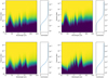 |
Fig. A.1 Contribution functions for the base spectra of each of the four planets considered in this study; HD 189733b (upper left), HD 209458b (upper right), HD 97658b (lower left), and Kepler-30c (lower right). |
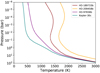 |
Fig. A.2 Pressure–temperature profiles of the four plants considered in this study, as determined from self-consistent temperaturestructure calculations using ARCiS (Min et al. 2020). |
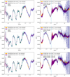 |
Fig. A.3 Simulated spectra (re-binned to R=100) for the atmospheres of a HD189733b-like planet observed with NIRISS SOSS and NIRSpec G395M (left column) and with NIRCam F322W2 and MIRI LRS (right column). The VMR was set to 10−6 for the hydrocarbon molecule specified in each legend for the simulated observed spectra. The best-fit retrieved spectra are given in orange for the cases where the molecule was removed, and in purple when it was included in the retrieval. The shading of the best-fit spectra corresponds to 1, 2, and 3 σ regions. |
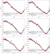 |
Fig. A.4 Zoomed-in section of simulated spectra (re-binned to R=100) for the atmospheres of a HD189733b-like planet observed with NIRISS SOSS and NIRSpec G395M (left column) and with NIRCam F322W2 and MIRI LRS (right column). The region illustrated is covered by both the NIRSpec G395M and NIRCam F322W2 instruments. The VMR was set to 10−6 for the hydrocarbon molecule specified in each legend for the simulated observed spectra. The best-fit retrieved spectra are given in orange for the cases where the molecule was removed, and in purple when it was included in the retrieval. The shading of the best-fit spectra corresponds to 1, 2, and 3 σ regions. |
References
- Baines, E. K., McAlister, H. A., ten Brummelaar, T. A., et al. 2008, ApJ, 680, 728 [NASA ADS] [CrossRef] [Google Scholar]
- Barman, T. S. 2007, ApJ, 661, L191 [NASA ADS] [CrossRef] [Google Scholar]
- Barstow, J. K. 2020, MNRAS, 497, 4183 [Google Scholar]
- Barstow, J. K., Aigrain, S., Irwin, P. G. J., Kendrew, S., & Fletcher, L. N. 2015, MNRAS, 448, 2546 [NASA ADS] [CrossRef] [Google Scholar]
- Barstow, J. K., Aigrain, S., Irwin, P. G. J., Kendrew, S., & Fletcher, L. N. 2016, MNRAS, 458, 2657 [NASA ADS] [CrossRef] [Google Scholar]
- Batalha, N., & Line, M. 2017, AJ, 153, 151 [NASA ADS] [CrossRef] [Google Scholar]
- Batalha, N., Kalirai, J., Lunine, J., Clampin, M., & Lindler, D. 2015, ArXiv e-prints [arXiv:1507.02655] [Google Scholar]
- Batalha, N., Mandell, A., Pontoppidan, K., et al. 2017, PASP, 129, 064501 [NASA ADS] [CrossRef] [Google Scholar]
- Benneke, B., & Seager, S. 2013, ApJ, 778, 153 [Google Scholar]
- Bernath, P. F. 2020, JQSRT, 240, 106687 [NASA ADS] [CrossRef] [Google Scholar]
- Bilger, C., Rimmer, P., & Helling, C. 2013, MNRAS, 435, 1888 [NASA ADS] [CrossRef] [Google Scholar]
- Birkby, J., de Kok, R., Brogi, M., et al. 2013, MNRAS, 436, L35 [NASA ADS] [CrossRef] [Google Scholar]
- Bouchy, F., Udry, S., Mayor, M., et al. 2005, A&A, 444, L15 [EDP Sciences] [Google Scholar]
- Boyajian, T., von Braun, K., Feiden, G. A., et al. 2014, MNRAS, 447, 846 [Google Scholar]
- Braam, M., van der Tak, F. F. S., Chubb, K. L., & Min, M. 2021, A&A, 646, A17 [NASA ADS] [CrossRef] [EDP Sciences] [Google Scholar]
- Brewer, J. M., Fischer, D. A., & Madhusudhan, N. 2017, AJ, 153, 83 [NASA ADS] [CrossRef] [Google Scholar]
- Brogi, M., Line, M., Bean, J., Désert, J.-M., & Schwarz, H. 2017, ApJ, 839, L2 [NASA ADS] [CrossRef] [Google Scholar]
- Burgdorf, M., Orton, G., van Cleve, J., Meadows, V., & Houck, J. 2006, Icarus, 184, 634 [NASA ADS] [CrossRef] [Google Scholar]
- Cabot, S. H. C., Madhusudhan, N., Hawker, G. A., & Gandhi, S. 2018, MNRAS, 482, 4422 [Google Scholar]
- Chubb, K. L., Tennyson, J., & Yurchenko, S. N. 2020, MNRAS, 493, 1531 [NASA ADS] [CrossRef] [Google Scholar]
- Chubb, K. L., Rocchetto, M., Al-Refaie, A. F., et al. 2021, A&A, 646, A17 [NASA ADS] [CrossRef] [EDP Sciences] [Google Scholar]
- Clark, R. N., Curchin, J. M., Barnes, J. W., et al. 2010, J. Geophys. Res. Planets, 115, E10 [Google Scholar]
- Coles, P. A., Yurchenko, S. N., & Tennyson, J. 2019, MNRAS, 490, 4638 [CrossRef] [Google Scholar]
- Cutri, R. M., Skrutskie, M. F., van Dyk, S., et al. 2003, VizieR Online Data Catalog: II/246 [Google Scholar]
- Dang, L., Cowan, N. B., Schwartz, J. C., et al. 2018, Nat. Astron., 2, 220 [NASA ADS] [CrossRef] [Google Scholar]
- de Kok, R., Brogi, M., Snellen, I., et al. 2013, A&A, 554, A82 [NASA ADS] [CrossRef] [EDP Sciences] [Google Scholar]
- Deming, D., & Seager, S. 2017, J. Geophys. Res. Planets, 122, 53 [NASA ADS] [CrossRef] [Google Scholar]
- Deming, D., Seager, S., Winn, J., et al. 2009, PASP, 121, 952 [NASA ADS] [CrossRef] [Google Scholar]
- Deming, D., Wilkins, A., McCullough, P., et al. 2013, ApJ, 774, 95 [Google Scholar]
- Drummond, B., Carter, A. L., Hébrard, E., et al. 2019, MNRAS, 486, 1123 [NASA ADS] [CrossRef] [Google Scholar]
- Eistrup, C., Walsh, C., & van Dishoeck, F. 2018, A&A, 613, A14 [NASA ADS] [CrossRef] [EDP Sciences] [Google Scholar]
- Fabrycky, D. C., Ford, E. B., Steffen, J. H., et al. 2012, ApJ, 750, 114 [Google Scholar]
- Feng, Y. K., Line, M. R., Fortney, J. J., et al. 2016, ApJ, 829, 52 [NASA ADS] [CrossRef] [Google Scholar]
- Feroz, F., & Hobson, M. P. 2008, MNRAS, 384, 449 [NASA ADS] [CrossRef] [Google Scholar]
- Feroz, F., Gair, J. R., Hobson, M. P., & Porter, E. K. 2009, Class. Quantum Gravity, 26, 215003 [NASA ADS] [CrossRef] [Google Scholar]
- Feroz, F., Hobson, M. P., Cameron, E., & Pettitt, A. N. 2019, Open J. Astrophys., 2, 10 [Google Scholar]
- Fortenbach, C., & Dressing, C. 2020, PASP, 132, 054501 [NASA ADS] [CrossRef] [Google Scholar]
- Gandhi, S., Brogi, M., Yurchenko, S. N., et al. 2020, MNRAS, 495, 224 [NASA ADS] [CrossRef] [Google Scholar]
- Gao, P., Thorngren, D. P., Lee, E. K. H., et al. 2020, Nat. Astron., 4, 951 [NASA ADS] [CrossRef] [Google Scholar]
- Giacobbe, P., Brogi, M., Gandhi, S., et al. 2021, Nature, 592, 205 [NASA ADS] [CrossRef] [Google Scholar]
- Gordon, I. E., Rothman, L. S., Hill, C., et al. 2017, JQSRT, 203, 3 [NASA ADS] [CrossRef] [Google Scholar]
- Greene,T., Beichman, C., Eisenstein, D., et al. 2007, Proc. SPIE, 6693, 153 [Google Scholar]
- Greene, T., Line, M. R., Montero, C., et al. 2016, AAS, 817, 17 [Google Scholar]
- Grootel, V. V., Gillon, M., Valencia, D., et al. 2014, ApJ, 786, 2 [NASA ADS] [CrossRef] [Google Scholar]
- Guilluy, G., Sozzetti, A., Brogi, M., et al. 2019, A&A, 625, A107 [NASA ADS] [CrossRef] [EDP Sciences] [Google Scholar]
- Guo, X., Crossfield, I. J. M., Dragomir, D., et al. 2020, AJ, 159, 239 [NASA ADS] [CrossRef] [Google Scholar]
- Guzmán-Mesa, A., Kitzmann, D., Fisher, C., et al. 2020, AJ, 160, 15 [Google Scholar]
- Harper, J. M., Helling, C., & Dufek, J. 2018, ApJ, 867, 123 [NASA ADS] [CrossRef] [Google Scholar]
- Hawker, G. A., Madhusudhan, N., Cabot, S. H. C., & Gandhi, S. 2018, ApJ, 863, L11 [NASA ADS] [CrossRef] [Google Scholar]
- Helling, C., Lee, E., Dobbs-Dixon, I., et al. 2016, MNRAS, 460, 855 [NASA ADS] [CrossRef] [Google Scholar]
- Hörst, S. M., Yoon, Y. H., Ugelow, M. S., et al. 2018, Icarus, 301, 136 [CrossRef] [Google Scholar]
- Howard, A. W., Johnson, J. A., et al. 2011, ApJ, 730, 10 [NASA ADS] [CrossRef] [Google Scholar]
- Howe, A., Burrows, A., & Deming, D. 2017, ApJ, 835, 96 [NASA ADS] [CrossRef] [Google Scholar]
- Hu, R., & Seager, S. 2014, ApJ, 784, 63 [Google Scholar]
- Kaltenegger, L., & Traub, W. 2009, ApJ, 698, 519 [NASA ADS] [CrossRef] [Google Scholar]
- Kawashima, Y., & Ikoma, M. 2019, ApJ, 877, 109 [NASA ADS] [CrossRef] [Google Scholar]
- Kawashima, Y., Hu, R., & Ikoma, M. 2019, ApJ, 876, L5 [Google Scholar]
- Kawashima, Yui, & Min, Michiel. 2021, A&A, 656, A90 [NASA ADS] [CrossRef] [EDP Sciences] [Google Scholar]
- Keles, E., Mallonn, M., von Essen, C., et al. 2019, MNRAS, 489, L37 [NASA ADS] [CrossRef] [Google Scholar]
- Knutson, H. A., Charbonneau, D., Cowan, N. B., et al. 2009, ApJ, 703, 769 [CrossRef] [Google Scholar]
- Knutson, H. A., Dragomir, D., Kreidberg, L., et al. 2014, ApJ, 794, 155 [Google Scholar]
- Kreidberg, L., Bean, J. L., Désert, J.-M., et al. 2014, ApJ, 793, L27 [Google Scholar]
- Lee, E., Dobbs-Dixon, I., Helling, C., Bognar, K., & Woitke, P. 2016, A&A, 594, A48 [NASA ADS] [CrossRef] [EDP Sciences] [Google Scholar]
- Li, G., Gordon, I. E., Rothman, L. S., et al. 2015, ApJS, 216, 15 [NASA ADS] [CrossRef] [Google Scholar]
- Lin, Z., MacDonald, R. J., Kaltenegger, L., & Wilson, D. J. 2021, MNRAS, 505, 3562 [NASA ADS] [CrossRef] [Google Scholar]
- Line, M. R., Stevenson, K. B., Bean, J., et al. 2016, AJ, 152, 203 [NASA ADS] [CrossRef] [Google Scholar]
- Lines, S., Mayne, N. J., Boutle, I. A., et al. 2018, A&A, 615, A97 [NASA ADS] [CrossRef] [EDP Sciences] [Google Scholar]
- Lombardo, N. A., Nixon, C. A., Achterberg, R. K., et al. 2019, Icarus, 317, 454 [NASA ADS] [CrossRef] [Google Scholar]
- MacDonald, R. J., & Madhusudhan, N. 2017, MNRAS, 469, 1979 [Google Scholar]
- MacDonald, R. J., Goyal, J. M., & Lewis, N. K. 2020, ApJ, 893, L43 [NASA ADS] [CrossRef] [Google Scholar]
- Maciejewski, G., Errmann, R., Raetz, S., et al. 2011, A&A, 528, A65 [NASA ADS] [CrossRef] [EDP Sciences] [Google Scholar]
- Macintosh, B., Graham, J. R., Barman, T., et al. 2015, Science, 350, 64 [Google Scholar]
- Madhusudhan, N. 2012, ApJ, 758, 36 [NASA ADS] [CrossRef] [Google Scholar]
- Mai, C., & Line, M. R. 2019, ApJ, 883, 144 [NASA ADS] [CrossRef] [Google Scholar]
- Mant, B. P., Yachmenev, A., Tennyson, J., & Yurchenko, S. N. 2018, MNRAS, 478, 3220 [NASA ADS] [CrossRef] [Google Scholar]
- McCullough, P., Stys, J., Valenti, J. A., et al. 2006, ApJ, 648, 1228 [NASA ADS] [CrossRef] [Google Scholar]
- McKay, C. P. 2016, Life, 6, 8 [NASA ADS] [CrossRef] [Google Scholar]
- McKemmish, L. K., Yurchenko, S. N., & Tennyson, J. 2016, MNRAS, 463, 771 [NASA ADS] [CrossRef] [Google Scholar]
- McKemmish, L. K., Masseron, T., Hoeijmakers, H. J., et al. 2019, MNRAS, 488, 2836 [Google Scholar]
- Miguel, Y., & Kaltenegger, L. 2014, ApJ, 780, 166 [Google Scholar]
- Min, M., Hovenier, J. W., & de Koter, A. 2005, A&A, 432, 909 [NASA ADS] [CrossRef] [EDP Sciences] [Google Scholar]
- Min, M., Ormel, C. W., Chubb, K., Helling, C., & Kawashima, Y. 2020, A&A, 642, A28 [NASA ADS] [CrossRef] [EDP Sciences] [Google Scholar]
- Molliére, P., van Boekel, R., Dullemond, C., Henning, T., & Mordasini, C. 2015, ApJ, 813, 47 [CrossRef] [Google Scholar]
- Molliére, P., van Boekel, R., Bouwman, J., et al. 2017, A&A, 600, A10 [CrossRef] [EDP Sciences] [Google Scholar]
- Moses, J., Bézard, B., Lellouch, E., et al. 2000, Icarus, 143, 244 [NASA ADS] [CrossRef] [Google Scholar]
- Moses, J. I., Madhusudhan, N., Visscher, C., & Freedman, R. S. 2012, ApJ, 763, 25 [Google Scholar]
- Nielsen, L. D., Ferruit, P., Giardino, G., et al. 2016, SPIE, 9904, 1218 [Google Scholar]
- Öberg, K. I., Murray-Clay, R., & Bergin, E. A. 2011, ApJ, 743, L16 [Google Scholar]
- Ormel, C. W., & Min, M. 2019, A&A, 622, A121 [NASA ADS] [CrossRef] [EDP Sciences] [Google Scholar]
- Pascale, E., Bezawada, N., Barstow, J., et al. 2018, SPIE, 10698, 169 [Google Scholar]
- Patapis, P., Nasedkin, E., Cugno, G., et al. 2022, A&A, 658, A72 [NASA ADS] [CrossRef] [EDP Sciences] [Google Scholar]
- Polyansky, O. L., Kyuberis, A. A., Zobov, N. F., et al. 2018, MNRAS, 480, 2597 [NASA ADS] [CrossRef] [Google Scholar]
- Rey, M., Nikitin, A. V., Babikov, Y. L., & Tyuterev, V. G. 2016, JMS, 327, 138 [Google Scholar]
- Rimmer, P. B., & Shorttle, O. 2019, Life, 9, 12 [CrossRef] [Google Scholar]
- Rimmer, P. B., Helling, C., & Bilger, C. 2014, Int. J. Astrobiol., 13, 173 [NASA ADS] [CrossRef] [Google Scholar]
- Rimmer, P. B., Ferus, M., Waldmann, I. P., et al. 2019, ApJ, 888, 21 [NASA ADS] [CrossRef] [Google Scholar]
- Rocchetto, M., Waldmann, I. P., Venot, O., Lagage, P.-O., & Tinetti, G. 2016, ApJ, 833, 120 [Google Scholar]
- Rothman, L. S., Gordon, I. E., Barber, R. J., et al. 2010, JQSRT, 111, 2139 [NASA ADS] [CrossRef] [Google Scholar]
- Sanchis-Ojeda, R., Fabrycky, D. C., Winn, J. N., et al. 2012, Nature, 487, 449 [Google Scholar]
- Schuler, S. C., Flateau, D., Cunha, K., et al. 2011, ApJ, 732, 55 [CrossRef] [Google Scholar]
- Sharpe, S., Sams, R., & Johnson, T. 2002, in AIPR ’02: Proc. 31st Applied Image Pattern Recognition Workshop on From Color to Hyperspectral: Advancements in Spectral Imagery Exploitation (IEEE Computer Society), 45 [CrossRef] [Google Scholar]
- Sinclair, J., Moses, J., Hue, V., et al. 2019, Icarus, 328, 176 [NASA ADS] [CrossRef] [Google Scholar]
- Sing, D. K., Fortney, J. J., Nikolov, N., et al. 2016, Nature, 529, 59 [Google Scholar]
- Sousa-Silva, C., Petkowski, J., & Seager, S. 2019, PCCP, 21, 18970 [NASA ADS] [CrossRef] [Google Scholar]
- Southworth, J. 2010, MNRAS, 408, 1689 [Google Scholar]
- Swain, M. R., Vasisht, G., & Tinetti, G. 2008, Nature, 452, 329 [NASA ADS] [CrossRef] [Google Scholar]
- Tarafdar, S. P., & Wickramasinghe, N. C. 1975, Ap&SS, 35, L41 [NASA ADS] [CrossRef] [Google Scholar]
- Taylor, J., Parmentier, V., Irwin, P. G. J., et al. 2020, MNRAS, 493, 4342 [NASA ADS] [CrossRef] [Google Scholar]
- Tennyson, J., & Yurchenko, S. 2018, Atoms, 6, 26 [CrossRef] [Google Scholar]
- Tennyson, J., Yurchenko, S. N., Al-Refaie, A. F., et al. 2020, JQSRT, 255, 107228 [NASA ADS] [CrossRef] [Google Scholar]
- Tielens, A. 2008, ARA&A, 46, 289 [Google Scholar]
- Torres, G., Winn, J. N., & Holman, M. J. 2008, ApJ, 677, 1324 [Google Scholar]
- Trotta, R. 2008, Contemp. Phys., 49, 71 [Google Scholar]
- Tsai, S.-M., Lyons, J. R., Grosheintz, L., et al. 2017, ApJS, 228, 20 [NASA ADS] [CrossRef] [Google Scholar]
- van Belle, G. T. 2008, PASP, 120, 617 [NASA ADS] [CrossRef] [Google Scholar]
- Venot, O., Hébrard, E., Agúndez, M., Decin, L., & Bounaceur, R. 2015, A&A, 577, A33 [NASA ADS] [CrossRef] [EDP Sciences] [Google Scholar]
- Waldmann, I. P., Tinetti, G., Rocchetto, M., et al. 2015, ApJ, 802, 107 [CrossRef] [Google Scholar]
- Woitke, P., Helling, C., Hunter, G. H., et al. 2018, A&A, 614, A1 [NASA ADS] [CrossRef] [EDP Sciences] [Google Scholar]
- Wunderlich, F., Scheucher, M., Godolt, M., et al. 2020, ApJ, 901, 126 [Google Scholar]
- Wyttenbach, A., Ehrenreich, D., Lovis, C., Udry, S., & Pepe, F. 2015, A&A, 577, A62 [NASA ADS] [CrossRef] [EDP Sciences] [Google Scholar]
- Yurchenko, S. N., Amundsen, D. S., Tennyson, J., & Waldmann, I. P. 2017, A&A, 605, A95 [NASA ADS] [CrossRef] [EDP Sciences] [Google Scholar]
- Yurchenko, S. N., Mellor, T. M., Freedman, R. S., & Tennyson, J. 2020, MNRAS, 496, 5282 [NASA ADS] [CrossRef] [Google Scholar]
- Zhang, M., Chachan, Y., Kempton, E. M.-R., & Knutson, H. A. 2019, PASP, 131, 034501 [CrossRef] [Google Scholar]
- Zilinskas, M., Miguel, Y., Molliére, P., & Tsai, S.-M. 2020, MNRAS, 494, 1490 [NASA ADS] [CrossRef] [Google Scholar]
All Tables
Abundances of various species computed assuming equilibrium chemistry and solar C/O and metallicity using GGCHEM (Woitke et al. 2018) at ~1.8 × 10⁻¹ bar.
Instrument and abundance set-ups for the models and retrievals of the four planets considered in this study.
Parameters and the corresponding ranges and priors used in the retrievals in this study.
Bayes factor (B01) for various retrievals for HD 189733b, which include a cloud deck at Ptop = 0.01 bar with a scattering slope of fmix = 1 × 10² × H2 scattering.
All Figures
|
Fig. 1 Comparison of transit spectra including increased hydrocarbon abundances, with respect to a base of equilibrium chemistry abundances for the main molecular species with the hydrocarbons removed. The spectra shown are for a planet modelled onKepler-30c, with an equilibrium temperature of 769 K. |
| In the text | |
|
Fig. 2 Cross sections of C2H2 computed using the ExoMol aCeTY line list (Chubb et al. 2020) for a range of temperatures at a pressure of 0.1 bar. |
| In the text | |
|
Fig. 3 Comparison of transmission spectra of a planet modelled on HD 189733b with varying hydrocarbon abundances. All species become visible at a VMR starting around 10−7. |
| In the text | |
|
Fig. 4 Base spectra (computed from equilibrium chemistry) of each of the four planet types used in this study, as detailed in each panel. Both the clear and the cloudy models for HD 189733b are included. Simulated JWST spectra and the corresponding error bars using PandExo are also plotted for each instrument used in this study (see figure legend). |
| In the text | |
|
Fig. 5 Posterior distributions from retrievals of model atmospheres of HD 189733b, HD 209458b, and HD 97658b for an input CH4 abundance of 10−4 (orange) andC2H2 and C2H4 in their respective equilibrium abundances (purple). The results using a variety of instruments are given. The model input abundance is indicated by a black line, which is not shown when lower than the presented range. |
| In the text | |
|
Fig. 6 Posterior distributions from retrievals of model atmospheres of HD 189733b, HD 209458b, and HD 97658b for an input CH4 abundance of 10−6 (orange) andC2H2 and C2H4 in their respective equilibrium abundances (purple). The results using a variety of instruments are given. The model input abundance is indicated by a black line, which is not shown when lower than the presented range. |
| In the text | |
|
Fig. 7 Posterior distributions from retrievals of model atmospheres of HD 189733b, HD 209458b, and HD 97658b for an input C2H2 abundance of 10−4 (orange) andC2H4 and CH4 in their respective equilibrium abundances (purple). The results using a variety of instruments are given. The model input abundance is indicated by a black line, which is not shown when lower than the presented range. |
| In the text | |
|
Fig. 8 Posterior distributions from retrievals of model atmospheres of HD 189733b, HD 209458b, and HD 97658b for an input C2H2 abundance of 10−6 (orange) andC2H4 and CH4 in their respective equilibrium abundances (purple). The results using a variety of instruments are given. The model input abundance is indicated by a black line, which is not shown when lower than the presented range. |
| In the text | |
|
Fig. 9 Posterior distributions from retrievals of model atmospheres of HD 189733b, HD 209458b, and HD 97658b for an input C2H4 abundance of 10−4 (orange) andC2H2 and CH4 in their respective equilibrium abundances (purple). The results using a variety of instruments are given. The model input abundance is indicated by a black line, which is not shown when lower than the presented range. |
| In the text | |
|
Fig. 10 Posterior distributions from retrievals of model atmospheres of HD 189733b, HD 209458b, and HD 97658b for an input C2H4 abundance of 10−6 (orange) andC2H2 and CH4 in their respective equilibrium abundances (purple). The results using a variety of instruments are given. The model input abundance is indicated by a black line, which is not shown when lower than the presented range. |
| In the text | |
|
Fig. 11 Posterior distributions from retrievals using selected combinations of instruments of model atmospheres of HD 189733b, HD 209458b, and HD 97658b for an input abundance of 10−4 for the main hydrocarbon specified (orange) and other species in their respective equilibrium abundances (purple). The model inputabundance is indicated by a black line, which is not shown when lower than the presented range. |
| In the text | |
|
Fig. 12 Retrieval results using NIRCam F322W2 and its combination, and NIRSpec G395M for HD 189733b when including clouds and a scattering slope, for increased C2H2 and C2H4 abundance to 10−6 (orange), respectively. The remaining species are in equilibrium abundance (purple) in each set of columns. The modelinput abundance is indicated by a black line, which is not shown when lower than the presented range. |
| In the text | |
|
Fig. 13 Posterior distributions from retrievals using 25 transits of model atmospheres of HD 97658b, for increased CH4 and C2H4 abundances of 10−6 (orange) and equilibrium abundance of the remaining species (purple). The model input abundance is indicated by a black line, which is not shown when lower than the presented range. |
| In the text | |
|
Fig. 14 Posterior distributions from retrievals using a variety of instruments for Kepler-30c, for increased CH4 abundance to 10−4 (orange) and equilibrium abundance for the remaining species (purple) in each set of columns. The model input abundance is indicated by a black line, which is not shown when lower than the presented range. |
| In the text | |
|
Fig. 15 Posterior distributions from retrievals using a variety of instruments and instrument combinations for Kepler-30c, for increased hydrocarbon abundances to 10−4 (orange) and equilibrium abundance for the remaining species (purple) in each set of columns. The model input abundance is indicated by a black line, which is not shown when lower than the presented range. |
| In the text | |
|
Fig. 16 Comparison of the observations for NIRCam F322W2 and NIRSpec G395M, for HD 209458b with CH4 increased to 10−6 (true spectrum), and C2H2 increased to 3⋅10−7 (as found from NIRSpec G395M observations). |
| In the text | |
|
Fig. A.1 Contribution functions for the base spectra of each of the four planets considered in this study; HD 189733b (upper left), HD 209458b (upper right), HD 97658b (lower left), and Kepler-30c (lower right). |
| In the text | |
|
Fig. A.2 Pressure–temperature profiles of the four plants considered in this study, as determined from self-consistent temperaturestructure calculations using ARCiS (Min et al. 2020). |
| In the text | |
|
Fig. A.3 Simulated spectra (re-binned to R=100) for the atmospheres of a HD189733b-like planet observed with NIRISS SOSS and NIRSpec G395M (left column) and with NIRCam F322W2 and MIRI LRS (right column). The VMR was set to 10−6 for the hydrocarbon molecule specified in each legend for the simulated observed spectra. The best-fit retrieved spectra are given in orange for the cases where the molecule was removed, and in purple when it was included in the retrieval. The shading of the best-fit spectra corresponds to 1, 2, and 3 σ regions. |
| In the text | |
|
Fig. A.4 Zoomed-in section of simulated spectra (re-binned to R=100) for the atmospheres of a HD189733b-like planet observed with NIRISS SOSS and NIRSpec G395M (left column) and with NIRCam F322W2 and MIRI LRS (right column). The region illustrated is covered by both the NIRSpec G395M and NIRCam F322W2 instruments. The VMR was set to 10−6 for the hydrocarbon molecule specified in each legend for the simulated observed spectra. The best-fit retrieved spectra are given in orange for the cases where the molecule was removed, and in purple when it was included in the retrieval. The shading of the best-fit spectra corresponds to 1, 2, and 3 σ regions. |
| In the text | |
Current usage metrics show cumulative count of Article Views (full-text article views including HTML views, PDF and ePub downloads, according to the available data) and Abstracts Views on Vision4Press platform.
Data correspond to usage on the plateform after 2015. The current usage metrics is available 48-96 hours after online publication and is updated daily on week days.
Initial download of the metrics may take a while.