| Issue |
A&A
Volume 699, July 2025
|
|
|---|---|---|
| Article Number | A97 | |
| Number of page(s) | 5 | |
| Section | Stellar atmospheres | |
| DOI | https://doi.org/10.1051/0004-6361/202554770 | |
| Published online | 04 July 2025 | |
Limb-darkening coefficients for four-term and power-2 laws for the JWST mission adopting spherical PHOENIX models at high resolution
NIRCam, NIRISS, and NIRSpec passbands
1
Instituto de Astrofísica de Andalucía, CSIC,
Apartado 3004,
18080
Granada,
Spain
2
Dept. Física Teórica y del Cosmos, Universidad de Granada,
Campus de Fuentenueva s/n,
10871
Granada,
Spain
3
Hamburger Sternwarte,
Gojenbergsweg 112,
21029
Hamburg,
Germany
4
Center for Astrophysics | Harvard & Smithsonian,
60 Garden St.,
Cambridge,
MA
02138,
USA
★ Corresponding author: This email address is being protected from spambots. You need JavaScript enabled to view it.
Received:
26
March
2025
Accepted:
21
May
2025
Abstract
Aims. Modeling observations of transiting exoplanets or close binary systems by comparing the observations with theoretical light curves requires precise knowledge of the distribution of specific intensities across the stellar disk. We aim to facilitate this type of research by providing extensive tabulations of limb-darkening coefficients for 11 frequently used near- and mid-infrared passbands on the NIRCam, NIRISS, and NIRSpec instruments installed on board the James Webb Space Telescope.
Methods. The calculation of the limb-darkening coefficients was based on spherically symmetric atmosphere models from the PHOENIX series, with a high spectral resolution (approximately 106 wavelengths), and covering the wavelength range 0.1-6.0 μm. The models were computed for solar composition, and a microturbulent velocity of 1.0 kms-1. We adopted two of the more accurate parametrizations for the coefficients: the four-term law, and the power-2 law. We applied the Levenberg-Marquardt least-squares minimization method, with a strategy to determine the critical value, μcrit, of the cosine of the viewing angle near the limb that is designed to improve numerical accuracy.
Results. The limb-darkening coefficients were derived based on a total of 306 atmosphere models covering an effective temperature range of 2400-7800 K, and a log g interval between 3.0 and 5.5. We discuss the quality of the fits to the specific intensities provided by the power-2 and four-term laws, as well as by the often-used quadratic law. Based on a comparison, we recommend the use of the four-term or power-2 laws, in that order of preference.
Key words: stars: atmospheres / binaries: eclipsing
© The Authors 2025
 Open Access article, published by EDP Sciences, under the terms of the Creative Commons Attribution License (https://creativecommons.org/licenses/by/4.0), which permits unrestricted use, distribution, and reproduction in any medium, provided the original work is properly cited.
This article is published in open access under the Subscribe to Open model. This email address is being protected from spambots. You need JavaScript enabled to view it. to support open access publication.
1 Introduction
Limb darkening is an important phenomenon in several areas of astrophysics research, including transiting extrasolar planets, eclipsing binary stars, spectroscopy, stellar microlensing events, interferometry, exozodiacal dust, line profiles of rotating stars, and many others. The correct treatment of this effect can be critical to the accuracy of the results, particularly in the present era of very high-precision observations made from space.
One of the first observations of the limb-darkening phenomenon was carried out centuries ago by Bouguer (1760). It was not until the beginning of the 20th century that theoretical research into the limb-darkening phenomenon began, led by Schwarzschild (1906). This author introduced a linear law to describe the distribution of specific intensities as a function of a parameter, μ = cos γ, where γ is the angle between the observer’s line of sight and the surface normal (see also Milne 1921). That well-known linear equation is written as
 (1)
(1)
where I(μ) is the specific intensity as a function of position on the stellar disc, and u is the linear limb-darkening coefficient (LDC). Some four decades later, Chandrasekhar (1944) and Placzek (1947) worked out some results concerning limb darkening for the grey atmosphere case.
A number of other laws with an extra term have been proposed since. For example, Kopal (2025) introduced the quadratic law
 (2)
(2)
which has been quite popular in recent years. A decade later, Van’t Veer (1960) proposed the following equation for the grey case:
 (3)
(3)
and Klinglesmith & Sobieski (1970) introduced the logarithmic law
 (4)
(4)
Another bi-parametric equation, the square-root law by Díaz-Cordovés & Giménez (1992), has the expression
 (5)
(5)
Compared to the linear formula, these bi-parametric laws yielded an improved agreement with the specific intensities provided by stellar atmosphere models, particularly in the case of Eq. (5) for stars with high effective temperatures. In the above equations, a, b1, e, and c are the linear LDCs, while b is the quadratic LDC, b3 the cubic LDC, f is the logarithmic LDC, and d the square-root LDC.
The best fit to model specific intensities provided by a biparametric law is due to Hestroffer (1997), who introduced a prescription that involves a power of μ, the so-called power-2 law. For a detailed discussion of the properties and advantages of this law, see Sections 3 and 4 of Claret & Southworth (2022). The power-2 law is expressed as
 (6)
(6)
where g and h are the corresponding LDCs.
More recently, Claret (2000) proposed a four-term nonlinear law written as
 (7)
(7)
in which ak are the associated LDCs. So far, this four-term limbdarkening prescription has achieved the best fits to the specific intensities from stellar atmosphere models, for both those using plane-parallel and spherical geometry.
Finally, Sing et al. (2009) advocated for an abbreviated form of the four-term law given by
 (8)
(8)
in which the μ1/2 term is omitted. Those authors pointed out that “The μ1/2 term from the four parameter nonlinear law mainly affects the intensity distribution at small μ values, and is not needed when the intensity at the limb varies approximately linearly at small μ values”. We note, however, that not all atmosphere models show a quasi-linear drop in intensity near the limb, to a degree that warrants the omission of that term. Models with non-negligible curvature include those based on spherical geometry, or those for hot stars (see our comment above regarding Eq. (5), which does include the μ1/2 term).
The advent of space missions has come with tighter requirements on precision in dealing with the phenomenon of limb darkening. Until recently, this was a concern mostly at optical wavelengths, where the effect is more noticeable. However, the launch of the James Webb Space Telescope (JWST) at the end of 2021 represents a significant advancement, among others, in our ability to explore the properties of exoplanets in the near-and mid-infrared, a region of the spectrum rich in new information. JWST has opened the door to detailed chemical studies of the complex atmospheres and compositions of these objects, through the analysis of light curves and/or transmission spectroscopy of unprecedented quality. These observations are now being gathered with the Near Infrared Camera (NIRCam), the Near Infrared Imager and Slitless Spectrograph (NIRISS), and the Near Infrared Spectrograph (NIRSpec) on board the spacecraft, as well as with the Mid Infrared Instrument (MIRI) at even longer wavelengths. To take full advantage of these new observations, proper treatment of limb darkening and other effects has become more important. The main goal of this work, therefore, is to facilitate the above studies by providing the community with tabulations of coefficients for the limb-darkening laws that match the intensity distribution of state-of-the-art atmosphere models with the highest fidelity.
With that in mind, we begin in Sect. 2 by mentioning a few of the recent observational results concerning exoplanets using the abovementioned instruments, in which limb darkening has played a role. We proceed then to Sect. 3, in which we describe the stellar atmosphere models used to generate the LDCs, as well as the numerical method we applied. LDCs are presented here for some of the most used passbands of NIRCam, NIRISS, and NIRSpec. We end with Sect. 4, in which we comment briefly on the quadratic limb-darkening law - one of the more popular ones in the exoplanet field - and its limitations.
2 Advances in transmission spectroscopy and light curve analyses using JWST
A large number of papers making use of the instruments installed on board JWST have appeared in recent literature, and many more are sure to come. In the very active field of exoplanets, some of those studies have dealt with the analysis of transit light curves or phase curves, and others with transmission spectroscopy. In both cases they rely on limb-darkening laws, in one way or another. To illustrate some of that work, below is a list of a few representative examples of such studies, along with the key results they have obtained:
Rustamkulov et al. (2023) analyzed the exoplanet WASP-39b, of a similar mass to Saturn, using the PRISM mode on JWST’s NIRSpec instrument. They report the detection of the following chemical species in the atmosphere of the planet: Na (19σ), H2O (33σ), CO2 (28σ), and CO (7σ).
Alderson et al. (2024) analyzed the super-Earth TOI-836b in the G395H passband of the NIRSpec instrument, and concluded that TOI-836b does not have an H2-dominated atmosphere.
Ahrer et al. (2023a) also investigated the exoplanet WASP-39b using NIRSpec/PRISM, and identified carbon dioxide (CO2) in its atmosphere. The same study detected water vapor, and placed a limit on the abundance of methane. They also concluded that the atmospheric metallicity is between 1 and 100 times solar.
Liu et al. (2025) studied the detectability of planetary oblateness, spin, and obliquity, from light curves obtained with NIRSpec/PRISM on JWST, using the exoplanet Kepler-167b as an example. They show that observations of a single transit would be able to detect a Saturn-like oblateness (f = 0.1) with high confidence, or set a stringent upper limit on the oblateness parameter, so long as the planetary spin is slightly misaligned (>20°) with respect to the orbital axis.
Feinstein et al. (2023) report an observation of the transmission spectrum of WASP-39b using the Single-Object Slitless Spectroscopy (SOSS) mode of the Near Infrared Imager. From their analysis of the atmosphere, they estimate the metallicity to be in the range of 10-30 times solar. They found a subsolar carbon-to-oxygen ratio, and a solar-to-super-solar potassium-to-oxygen ratio.
Lustig-Yaeger et al. (2023) used NIRSpec in the G395H passband to validate and study the Earth-sized exoplanet LHS 475b. They rule out primordial hydrogen-dominated and cloudless pure methane atmospheres.
Wallack et al. (2024) investigated the spectrum of the sub-Neptune TOI-836c using the G395H passband of NIR-Spec. The authors rule out atmospheric metallicities below 175 times solar in the absence of aerosols at <1 millibar.
The above investigations, and many others like them that take advantage of the observational capabilities of the JWST mission, provide the motivation for supplying users with new LDCs for the four-term and power-2 laws, covering 11 passbands used with the NIRCam, NIRISS, and NIRSpec instruments. The limitations of other limb-darkening parametrizations have been pointed out in some of the above studies (e.g., Ahrer et al. 2023), and we expect the new coefficients calculated here to bring improvements in the analysis of observational data from this space mission.
3 Stellar atmosphere models and methodology
In this paper we made use of state-of-the-art spherically symmetric models based on the PHOENIX code (NewEra model grid; Hauschildt et al. 2025). A 1D spherically symmetric model can be described loosely as being made up of two parts: a core and an envelope. Roughly speaking, the core behaves approximately as prescribed by a plane-parallel model. The envelope behaves differently, as it carries the spherical part. We define quasi-spherical models as ones that do not consider the full intensity drop-off region. This concept is useful for situations in which small intensities near the limb coming from spherical models cannot be observationally detected, and/or if the effects of sphericity are negligible.
Here we employ the Levenberg-Marquardt least-squares minimization method (LML), adapted to the nonlinear case to derive the LDCs for these models. Before applying the LML to each passband, the specific intensities for the photometric systems of interest were integrated using the following equation:
 (9)
(9)
In this expression h is the Planck constant, λ is the wavelength, c is the speed of light in vacuum, Ia(μ) is the specific intensity in passband a, I(λ, μ) is the monochromatic specific intensity, and S (λ)a is the response function. Table 1 lists the JWST passbands considered for this work, and their mean wavelengths1.
The LDC calculations were performed for a total of 306 PHOENIX models specifically computed for the present work, with each atmosphere model occupying more than 2.0 GB of disc space. In order to improve the input physics for the analysis of light curves and transmission spectroscopy, the models were originally computed at very high resolution, with approximately 1.08 × 10⁶ wavelength points covering the range 0.1-6.0 μm that is relevant for the JWST passbands of NIRCam, NIRISS, and NIRSpec. All models were calculated for the solar abundance and a fixed microturbulent velocity of ξ = 1.0 km s-1 (as per Hauschildt et al. 2025), over an interval in surface gravity, log g, between 3.0 to 5.5, and effective temperatures, Teff, from 2400 to 7800 K. In each case, we interpolated the original grid of 127 μ locations to form 60 000 regularly spaced points, in order to better sample the limb of the star and avoid numerical inaccuracies that would otherwise occur when using LML.
The specific intensities from spherical model atmospheres show a much more pronounced curvature near the limb than their plane-parallel model counterparts. In fact, the specific intensity for spherical models drops to zero. For this reason, it is more challenging to obtain good fits in that region with some of the simpler limb-darkening laws mentioned earlier. Only more flexible ones, such as the four-term law, are able to provide acceptable fits for the entire intensity profile, although even for that prescription some of the passbands yield less than optimal fits (see, e.g., Fig. 1 by Claret et al. 2012).
In an earlier attempt to better describe the intensity distributions, Claret & Hauschildt (2003) introduced the concept of quasi-spherical models. However, this simple approach only takes into account the points in the intensity profile before the drop-off, down to an arbitrarily chosen value of μ referred to as the critical point, μcrit, which is the smallest value used in fitting a given limb-darkening law. A year later, Wittkowski et al. (2004) introduced a more sophisticated approach, whereby instead of relying on an arbitrarily selected critical point they defined it as the value of μ corresponding to the maximum of the derivative of the specific intensity with respect to r, where  . This point corresponds to a Rosseland mean optical depth of τR ≈ 1.0. The present PHOENIX models were computed with sufficient μ sampling in the drop-off region to allow us to determine the required derivative more precisely. Here we adopt the methodology of Wittkowski et al. (2004), which produces steeper profiles and is therefore more difficult to adjust, but provides a better representation of the spherical part of the atmosphere models. The merit function used as a measure of the quality of the fit for each passband is
 (10)
(10)
where yi is the model intensity at point i, Yi is the fitted function at the same point, and N is the number of μ points.
The LDCs calculated for the four-term law are presented in Table 2 for all passbands, and those for the power-2 law in Table 3. Both are available at the CDS.
As an illustration, Figs. 1 and 2 present comparisons of the fits to the intensity profile for the four-term and the power-2 laws, for two of the NIRISS passbands. Plots for the other passbands in Table 1 are similar. In general, the fits with the four-term law give smaller χ2 values than those with the power-2 law. In some cases the χ2 values from the four-term law can be up to 100 times smaller, while in others they are similar. A graphical comparison of the fit qualities between the four-term, power-2, and quadratic laws is shown in Figs. 3-5.
NIRCam, NIRISS, and NIRSpec passbands.
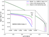 |
Fig. 1 Angular distribution of the specific intensity for a model with Teff = 5800 K, log g = 4.5, [M/H] = 0.0, and ξ = 1.0 km s-1 (blue line), for the NIRISS SOSS Order 2 passband. The fits provided by the four-term and power-2 laws are displayed for comparison. The inset shows an enlargement around the drop-off region. |
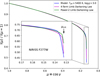 |
Fig. 2 Similar to Fig. 1, for a model with Teff = 5400 K, log g = 3.0, [M/H] = 0.0, and ξ = 1.0 km s-1 (blue line). The NIRISS passband shown here is F277W. |
4 Final remarks
Among the bi-parametric limb-darkening laws, the quadratic formula (Eq. (2)) is one of the most commonly used in the literature for the analysis of light curves and transmission spectroscopy. We point out, however, that this prescription generally does not provide accurate fits to the specific intensities produced by realistic atmosphere models, for any given Teff, log g, or metallicity. This is the case even for models that adopt plane-parallel geometry (Claret & Southworth 2022; see their Figs. 2 and 3). The χ2 values associated with such fits are quite high, and the flux is not conserved within reasonable limits. See Figs. 3-5, where we compare the qualities of the fits among the quadratic, power-2, and four-term laws. Use of the quadratic prescription runs the risk of implicitly introducing into the analysis a model of the stellar atmosphere that is not a good representation of the one we intended to begin with, characterized by certain values of Teff, log g, metallicity, and microturbulent velocity. As a result, significant biases can be introduced into the analysis of high-precision data such as that which JWST provides. Similar comments have been made recently by Coulombe et al. (2024). In reality, of course, none of the three laws mentioned previously (four-term, power-2, quadratic) achieve a perfect fit to the distribution of specific intensities, as they are only convenient approximations. However, based on the results of this paper, and others discussing limb darkening, it is advisable to avoid using the quadratic law. Instead, here we recommend the four-term or power-2 laws, in that order of preference. The LDCs computed in this work for the 11 JWST passbands are available at the CDS: Table 2 (four-term formula) and Table 3 (power-2 formula). Additional calculations can be carried out on request for other photometric systems that are within the mentioned spectral range of the present models.
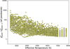 |
Fig. 3 Comparison of the quality of the fits for all passbands studied here. The quality metric shown is the ratio between the χ2 values computed using the quadratic law and the power-2 law, for all 306 models. |
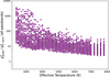 |
Fig. 4 Similar to Fig. 3, for the ratio between the χ2 values computed using the quadratic law and the four-term law. |
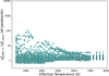 |
Fig. 5 Similar to Fig. 3, for the ratio between the χ2 values computed using the power-2 law and the four-term law. |
Data availability
Tables 2 and 3 are available at the CDS via anonymous ftp to cdsarc.cds.unistra.fr (130.79.128.5) or via https://cdsarc.cds.unistra.fr/viz-bin/cat/J/A+A/699/A97
Acknowledgements
We thank the anonymous referee for helpful comments. The Spanish MINC/AEI (PID2022-137241NB-C43 and PID2019-107061GB-C64) are gratefully acknowledged for their support during the development of this work. We also thank R. Morales and N. Robles (UDIT-IAA-CSIC) for their assistance with the calculations. A.C. also acknowledges financial support from grant CEX2021-001131-S, funded by MCIN/AEI/10.13039/501100011033.
The model grid calculations presented here were partially performed at the National Energy Research Supercomputer Center (NERSC), which is supported by the Office of Science of the U.S. Department of Energy under Contract No. DE-AC03-76SF00098. The authors gratefully acknowledge the computing time made available to them on the high-performance computers HLRN-IV at GWDG at the NHR Center NHR@Göttingen and at ZIB at the NHR Center NHR@Berlin. These Centers are jointly supported by the Federal Ministry of Education and Research, and the state governments participating in the NHR (www.nhr-verein.de/unsere-partner). Additional computing time was provided by the RRZ computing clusters Hummel and Hummel2. We thank all of these institutions for a generous allocation of computer time. This research has made use of the SIMBAD database, operated at the CDS, Strasbourg, France, and of NASA’s Astrophysics Data System Abstract Service.
References
- Alderson, L., Batalha, N. E., Wakeford, H. R., et al. 2024, AJ, 167, 216 [Google Scholar]
- Ahrer, E-M., Alderson, L., Batalha, N. M., et al., 2023a, Nature, 614, 649 [Google Scholar]
- Ahrer, E-M., Stevenson, K. B., Mansfield, M., et al., 2023b, Nature, 614, 653 [Google Scholar]
- Bouguer, P., 1760, Traité d’Optique, l’Abbé de la Caille (Smithsonian Miscellaneous Collections: Paris) [Google Scholar]
- Chandrasekhar, S. 1944, ApJ, 99, 180 [Google Scholar]
- Claret, A. 2000, A&A, 363, 1081 [NASA ADS] [Google Scholar]
- Claret, A., & Hauschildt, P. H. 2003, A&A 412, 241 [NASA ADS] [CrossRef] [EDP Sciences] [Google Scholar]
- Claret, A., & Southworth, J. 2022, A&A, 664, A128 [NASA ADS] [CrossRef] [EDP Sciences] [Google Scholar]
- Claret, A., Hauschildt, P. H., & Witte, S. 2012, A&A, 546, 14 [Google Scholar]
- Coulombe, L.-P., Roy, P.-A., & Benneke, B. 2024, AJ, 168, 227 [Google Scholar]
- Díaz-Cordovés, J., & Giménez, A. 1992, A&A, 259, 227 [NASA ADS] [Google Scholar]
- Feinstein, A. D., Radica, M., Welbanks, L., et al. 2023, Nature, 614, 670 [NASA ADS] [CrossRef] [Google Scholar]
- Hauschildt, P. H., Barman, T., Baron, E., et al. 2025, A&A, 698, A47 [NASA ADS] [CrossRef] [EDP Sciences] [Google Scholar]
- Hestroffer, D. 1997, A&A, 327, 199 [NASA ADS] [Google Scholar]
- Klinglesmith, D. A., & Sobieski, S. 1970, AJ, 75, 175 [Google Scholar]
- Kopal, Z. 1950, Harvard College Observ. Circ., 454, 1 [Google Scholar]
- Liu, Q., Zhu, W., Zhou, Y., et al. 2025 AJ, 169, 79 [Google Scholar]
- Lustig-Yaeger, J., Fu, G., May, E. M. 2023, Nat. Astron., 7, 1317 [NASA ADS] [CrossRef] [Google Scholar]
- Milne, E. A. 1921, MNRAS, 81, 361 [Google Scholar]
- Placzek, G. 1947, Phys. Rev. 72, 556 [Google Scholar]
- Rustamkulov, Z., Sing, D. K., Mukherjee, S., et al. 2023, Nature, 614, 659 [NASA ADS] [CrossRef] [Google Scholar]
- Sing, D. K., Désert, J., Lecavelier Des Etangs, A., et al. 2009, A&A, 505, 891 [NASA ADS] [CrossRef] [EDP Sciences] [Google Scholar]
- Schwarzschild, K. 1906, Nachrichten von der Gesellschaft der Wissenschaften zu Göttingen, Mathematisch-Physikalische Klasse, 43 [Google Scholar]
- Van’t Veer, F. 1960, Rech. Astr. Obs. Utrecht, 14, 3 [Google Scholar]
- Wallack, N. L., Batalha, N., Alderson, L., et al. 2024, AJ, 168, 77 [NASA ADS] [CrossRef] [Google Scholar]
- Wittkowski, M., Aufdenberg, J. P., & Kervella, P. 2004, A&A, 413, 711 [NASA ADS] [CrossRef] [EDP Sciences] [Google Scholar]
The corresponding transmission functions for these and other JWST passbands can be obtained at https://jwst-docs.stsci.edu/jwst-exposure-time-calculator-overview/jwst-etc-pandeia-engine-tutorial/jwst-etc-instrument-throughputs#gsc.tab=0, and plots can be generated at https://jwst.etc.stsci.edu/
All Tables
All Figures
|
Fig. 1 Angular distribution of the specific intensity for a model with Teff = 5800 K, log g = 4.5, [M/H] = 0.0, and ξ = 1.0 km s-1 (blue line), for the NIRISS SOSS Order 2 passband. The fits provided by the four-term and power-2 laws are displayed for comparison. The inset shows an enlargement around the drop-off region. |
| In the text | |
|
Fig. 2 Similar to Fig. 1, for a model with Teff = 5400 K, log g = 3.0, [M/H] = 0.0, and ξ = 1.0 km s-1 (blue line). The NIRISS passband shown here is F277W. |
| In the text | |
|
Fig. 3 Comparison of the quality of the fits for all passbands studied here. The quality metric shown is the ratio between the χ2 values computed using the quadratic law and the power-2 law, for all 306 models. |
| In the text | |
|
Fig. 4 Similar to Fig. 3, for the ratio between the χ2 values computed using the quadratic law and the four-term law. |
| In the text | |
|
Fig. 5 Similar to Fig. 3, for the ratio between the χ2 values computed using the power-2 law and the four-term law. |
| In the text | |
Current usage metrics show cumulative count of Article Views (full-text article views including HTML views, PDF and ePub downloads, according to the available data) and Abstracts Views on Vision4Press platform.
Data correspond to usage on the plateform after 2015. The current usage metrics is available 48-96 hours after online publication and is updated daily on week days.
Initial download of the metrics may take a while.