| Issue |
A&A
Volume 658, February 2022
|
|
|---|---|---|
| Article Number | A93 | |
| Number of page(s) | 10 | |
| Section | Planets and planetary systems | |
| DOI | https://doi.org/10.1051/0004-6361/202142327 | |
| Published online | 04 February 2022 | |
OGLE-2019-BLG-0468Lb,c: Two microlensing giant planets around a G-type star
1
Department of Physics, Chungbuk National University,
Cheongju
28644,
Republic of Korea
e-mail: cheongho@astroph.chungbuk.ac.kr
2
Astronomical Observatory, University of Warsaw,
Al. Ujazdowskie 4,
00-478 Warszawa,
Poland
3
Korea Astronomy and Space Science Institute,
Daejon
34055,
Republic of Korea
4
Department of Astronomy and Tsinghua Centre for Astrophysics, Tsinghua University,
Beijing
100084,
PR China
5
University of Canterbury, Department of Physics and Astronomy,
Private Bag 4800,
Christchurch
8020, New Zealand
6
Korea University of Science and Technology,
217 Gajeong-ro,
Yuseong-gu,
Daejeon
34113, Republic of Korea
7
Max Planck Institute for Astronomy,
Königstuhl 17,
69117
Heidelberg,
Germany
8
Department of Astronomy, The Ohio State University,
140 W. 18th Ave.,
Columbus,
OH
43210, USA
9
Department of Particle Physics and Astrophysics, Weizmann Institute of Science,
Rehovot
76100,
Israel
10
Center for Astrophysics, Harvard & Smithsonian 60 Garden St.,
Cambridge,
MA 02138,
USA
11
School of Space Research, Kyung Hee University,
Yongin,
Kyeonggi
17104, Republic of Korea
12
Department of Astronomy & Space Science, Chungbuk National University,
Cheongju
28644,
Republic of Korea
13
Department of Physics & Astronomy, Seoul National University,
Seoul
08826,
Republic of Korea
14
Division of Physics, Mathematics, and Astronomy, California Institute of Technology,
Pasadena,
CA
91125, USA
15
Department of Physics, University of Warwick,
Gibbet Hill Road,
Coventry,
CV4 7AL, UK
16
South African Astronomical Observatory,
PO Box 9,
Observatory
7935,
Cape Town, South Africa
17
Kavli Institute for Astronomy and Astrophysics, Peking University,
Beijing
100871,
PR China
18
National Astronomical Observatories, Chinese Academy of Sciences,
Beijing
100012,
PR China
Received:
29
September
2021
Accepted:
5
November
2021
Aims. With the aim of interpreting anomalous lensing events with no suggested models, we conducted a project of reinvestigating microlensing data collected in and before the 2019 season. In this work, we report a multi-planet system, OGLE-2019-BLG-0468L, that was found as a result of this project.
Methods. The light curve of the lensing event OGLE-2019-BLG-0468, which consists of three distinctive anomaly features, could not be explained by the usual binary-lens or binary-source interpretations. We find a solution that explains all anomaly features with a triple-lens interpretation, in which the lens is composed of two planets and their host, making the lens the fourth multi-planet system securely found by microlensing.
Results. The two planets have masses of ~3.4 MJ and ~10.2 MJ, and they are orbiting around a G-type star with a mass of ~0.9 M⊙ and a distance of ~4.4 kpc. The host of the planets is most likely responsible for the light of the baseline object, although the possibility of the host being a companion to the baseline object cannot be ruled out.
Key words: gravitational lensing: micro / planets and satellites: detection
© ESO 2022
1 Introduction
Studies based on radial velocity (RV) observations have shown that beyond ~1 AU about 10% of stars have giant planets (Cumming et al. 2008; Fulton et al. 2021). One question to ask is how common it is for such cold giant planets to have massive planetary-mass companions. On one hand, cold giant planets have eccentric orbits that are generally attributed to dynamical interactions with additional massive companions, suggesting that perhaps the majority of them have such companions, at least at birth (Jurić & Tremaine 2008; Chatterjee et al. 2008). On the other hand, after over two decades of searches, RV surveys have only been able to identify the presence of massive companions to ~20–30% of known cold giants (Wright et al. 2009; Rosenthal et al. 2021). This discrepancy can potentially be reduced with more discoveries of giant planet systems, but unfortunately RV becomes extremely inefficient in detecting planets with relatively low masses and/or long orbital periods.
Being most sensitive to cold planets located around or beyond the water snow line, gravitational microlensing can play an important role in completing the demographic census of exoplanets (Gaudi 2012; Zhu & Dong 2021). In terms of multi-planet systems, microlensing has so far detected three reliable two-planet systems, OGLE-2006-BLG-109L (Gaudi et al. 2008; Bennett et al. 2010), OGLE-2012-BLG-0026L (Han et al. 2013; Beaulieu et al. 2016), and OGLE-2018-BLG-1011L (Han et al. 2019), in addition to two candidate two-planet systems, OGLE-2014-BLG-1722L (Suzuki et al. 2018) and KMT-2019-BLG-1953L (Han et al. 2020a). Compared to the total number of over 100 planetary systems found with microlensing, the number of multi-planet systems is small. However, given the relatively low efficiency of detecting multi-planet systems with microlensing (Zhu et al. 2014), these numbers already somewhat indicate that a perhaps substantial fraction of microlensing planets have additional planetary-mass companions (Madsen & Zhu 2019).
Given the potential of microlensing in studying the multiplicity distribution of cold planets and thus the architecture of planetary systems in the cold region, it is important to detect more, secure multi-planet microlensing systems. This requires high-cadence observations over a large number of microlensing events as well as detailed light curve modelings of all anomalous events. The signal produced by multiple planets differs from that produced by a single planet because the individual planets induce their own caustics and these caustics often result in a complex pattern due to the interference between the caustics (Daněk & Heyrovský 2015a,b, 2019). As a result, these signals, in most cases, cannot be described by the usual lensing models based on the binary-lens (2L1S) or binary-source (1L2S) interpretations. This implies that some anomalous events with signals produced by multiple planets are probably left unanalyzed.
The amount of microlensing data was dramatically decreased during the COVID-19 pandemic because many of the major survey telescopes were shut down. In order to make the best use of this downtime, we conducted a project in which previous microlensing data collected by the Korea Microlensing Telescope Network (KMTNet) survey in and before the 2019 season were systematically reinvestigated. The aim of the project is to find events of scientific importance among those with no presented analyses. One group of events for this investigation are those with weak anomalies. Investigating such events led to the discoveries of 16 microlensing planets: KMT-2018-BLG-1025Lb (Han et al. 2021e), KMT-2016-BLG-2364Lb, KMT-2016-BLG-2397Lb, OGLE-2017-BLG-0604Lb, OGLE-2017-BLG-1375Lb (Han et al. 2020e), KMT-2018-BLG-0748Lb (Han et al. 2020d), KMT-2019-BLG-1339Lb (Han et al. 2020b), KMT-2018-BLG-1976, KMT-2018-BLG-1996, OGLE-2019-BLG-0954 (Han et al. 2021d), OGLE-2018-BLG-0977Lb, OGLE-2018-BLG-0506Lb, OGLE-2018-BLG-0516Lb, OGLE-2019-BLG-1492Lb, KMT-2019-BLG-0253 (Hwang et al. 2022), and OGLE-2019-BLG-1053 (Zang et al. 2021).
Another group of targeted events are those with known anomalies but for which interpretations of the anomalies have not been presented. From the investigation of such events, it was found that KMT-2019-BLG-1715 was a planetary event involved with three lens masses and two source stars (Han et al. 2021c), KMT-2019-BLG-0797 was a binary-lensing event occurring on a binary stellar system, a 2L2S event (Han et al. 2021b), and KMT-2019-BLG-1953 was a strong candidate planetary event with a lens composed of two planets and the host (Han et al. 2020a). The events in this group have the common characteristic that interpreting the lensing light curves of the events requires one to add extra source or lens components into the modeling.
In this work we present the results found from the reanalysis of the lensing event OGLE-2019-BLG-0468. The light curve of the event was previously investigated with 2L1S and 1L2S interpretations, but no plausible solution was suggested. From the reanalysis of the event based on more sophisticated models, we find that the event was produced by a triple-lens (3L1S) system, in which the lens is composed of two giant planets and their host star.
We present the analysis of the event according to the following organization. In Sect. 2 we describe observations of the lensing event and the characteristics of the observed light curve. In Sect. 3 we depict various models tested to explain the observed light curve, including 2L1S, 1L2S, 2L2S, and 3L1S models. In Sect. 4 we characterize the source star and estimate the angular Einstein radius. In Sect. 5 we estimate the physical lens parameters using the available observables of the event. In Sect. 6 we discuss the possibility that the baseline object is the lens. We then summarize our results and conclude in Sect. 7.
2 Observations and data
The source of the lensing event OGLE-2019-BLG-0468 lies in the Galactic bulge field at the equatorial coordinates  17:45:37.44, − 24:26:50.2), which correspond to the Galactic coordinates (l, b) = (3°.834, 2°.336). The apparent baseline I-band magnitude of the source is Ibase = 17.8 according to the Optical Gravitational Lensing Experiment IV (OGLE-IV) photometry system. As we show in Sect. 4, the source is much fainter than the baseline magnitude, and the baseline flux comes mostly from a blend.
Figure 1 shows the light curve of OGLE-2019-BLG-0468. The rising of the source flux induced by lensing was first found by the OGLE-IV (Udalski et al. 2015) survey in the early part of the 2019 season, on April 13, 2019 (HJD′≡HJD − 2 450 000 ~ 8586). The OGLE teamutilizes the 1.3 m telescope at the Las Campanas Observatory in Chile, which is equipped with a camera that yields a 1.4 deg2 field of view. The source flux increased until t1 ~ 8586.3 and then declined during 8586 ≲HJD′≲ 8590, producing a weak bump at around t1. The flux suddenly increased at t2 ~ 8592.9, suggesting that the source crossed a caustic induced by the multiplicity of the lens. The detailed structure of the light curve for the three nights during the period 8596 ≲HJD′≲ 8598 could not bedelineated because the OGLE observation of the event was not conducted for that time. When the event was observed by the OGLE survey againon HJD′~ 8599, the source flux continued to decline until it reached the baseline.
The event was also located in the field covered by the KMTNet survey (Kim et al. 2016). The KMTNet group utilizes three identical telescopes, each of which has a 1.6 m aperture and is mounted with a camera that yields a 4 deg2 field of view. For the continuous coverage of lensing events, the telescopes are distributed over the three continents of the Southern Hemisphere, at the Siding Spring Observatory in Australia (KMTA), the Cerro Tololo Inter-American Observatory in Chile (KMTC), and the South African Astronomical Observatory in South Africa (KMTS). For both the OGLE and KMTNet surveys, observations of the event were done mainly in the I band, and a fraction of V -band images wereacquired for the measurement of the source color. The event was identified by the KMTNet survey from the post-season inspection of the 2019 season data, and it was labeled as KMT-2019-BLG-2696. Hereafter we use only the OGLE event number, according to the order of discovery, to designate the event. The light curve constructed with the additional KMTNet data revealed that there existed an additional peak at t3 ~ 8595.7 that was not covered by the OGLE data. Figure 2 shows the zoomed-in view of the light curve around the epochs t2 and t3.
The light curve of the event was constructed by conducting photometry of the source using the pipelines of the individual survey groups: Woźniak (2000) for OGLE and Albrow et al. (2009) for KMTNet. In order to consider the scatter of the data and to make χ2 per degree of freedom for each data set unity, the error bars estimated by the pipelines were readjusted according to the prescription depicted in Yee et al. (2012).
In addition to the photometric data, we also obtained two spectra, with a 1000 s exposure for each, of the baseline object on the night of June 3, 2021(HJD′ = 9398), which is ~2.2 yr after the event, using the Robert Stobie Spectrograph (Burgh et al. 2003) mounted on the South African Large Telescope (SALT; Buckley et al. 2006). The spectroscopic data were reduced using a custom pipeline based on the PySALT package (Crawford et al. 2010), which accounts for basic charge-coupled device characteristics, removal of cosmic rays, wavelength calibration, and relative flux calibration. To estimate the stellar parameters (Teff, log g, and [Fe/H]), we interpolated the observed spectra in an empirical grid (Du et al. 2019), which was constructed with massive spectra collected by the Large Sky Area Multi-Object Fibre Spectroscopic Telescope (LAMOST). Unfortunately, it was difficult to securely estimate the stellar parameters due to the low signal-to-noise ratios of the spectra.
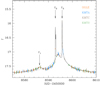 |
Fig. 1 Light curve of the microlensing event OGLE-2019-BLG-0468. The arrows labeled t1 (8586.3), t2 (8592.9), and t3 (8595.7) indicate the three epochs of major anomalies. The curves drawn over the data points represent the 1L1S (dotted curve) and 3L1S (close-close model, solid curve) models. The zoomed-in view of the anomaly region around t2 and t3 is shown in Fig. 2. |
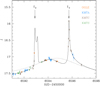 |
Fig. 2 Zoomed-in view of the anomaly region around the epochs t2 and t3. Notations are the same as in Fig. 1. |
3 Light curve interpretation
3.1 2L1S, 1L2S, and 2L2S models
We first modeled the observed light curve under the assumption of lens (2L1S model) or source (1L2S model) binarity, which is the most common cause of lensing light curve anomalies. The lensing light curve of a single-lens single-source (1L1S) event is characterized by the three parameters (t0, u0, tE), which represent the time of the closest lens-source approach, the lens-source separation at t0, and the event timescale, respectively. Adding an extra lens or source component into the modeling requires one to include extra parameters. For a 2L1S event, these extra parameters are (s, q, α), which denote the binary separation, the mass ratio between the lens components, and the angle between the direction of the source motion and the binary axis (source trajectory angle), respectively. For a 1L2S event, the extra parameters are (t0,2, u0,2, qF), the first two of which are the closest approach time and separation of the source companion, and the last parameter indicates the flux ratio between the companion (S2) and primary (S1) source stars. In all cases of the tested models, we included an additional parameter, ρ, which denotes the ratio of the angular source radius, θ*, to the angular Einstein radius, θE, that is, ρ = θ*∕θE (normalized source radius), to account for possible finite-source effects in the lensing light curve. To distinguish parameters related to S1 and S2, we use the notations (t0,1, u0,1, ρ1) and (t0,2, u0,2, ρ2), respectively.
From the modeling of the observed light curve with the 2L1S and 1L2S interpretations, it was found that the data cannot be explained by these models. In Fig. 3 we plot the model curves and residuals of the 2L1S (dashed curve) and 1L2S (dot-dashed curve) models. The lensing parameters of these models are listed in Table 1 together with the χ2 values of the fits.
We made an additional check with a 2L2S model, in which both the lens and source are binaries; such a system is exemplified by MOA-2010-BLG-117 (Bennett et al. 2018), OGLE-2016-BLG-1003 (Jung et al. 2017), KMT-2019-BLG-0797 (Han et al. 2021b), and KMT-2018-BLG-1743 (Han et al. 2021a). The model curve and residual from the 2L2S solution are presented in Fig. 3, and the lensing parameters of the solution are listed inTable 1. This model provides a better fit than the 2L1S and 1L2S models by Δχ2 = 295.2 and 2069.7, respectively. However, the model still leaves substantial residuals, indicating that a new interpretation of the light curve is needed.
3.2 3L1S model
We then tested a model in which the lens is a triple system (3L1S model). In the first step of this modeling, we checked whether a 2L1S model can describe part of the anomalies, although it turned out that the model could not explain all anomaly features. We did this check because lensing light curves with three lens components (M1, M2, and M3) can, in many cases, be approximated by the superposition of two 2L1S light curves produced by M1 –M2 and M1 –M3 lens pairs (Bozza 1999; Han et al. 2001). This is exemplified by the light curve of OGLE-2012-BLG-0026 (Han et al. 2013), which is generated by a lens composed of two planets and a host star, and that of OGLE-2018-BLG-1700 (Han et al. 2020c), which is produced by a lens composed of a planet and binary stars. From the modeling conducted with the partial data, excluding those after t2, it is found that the light curve is well approximated by a 2L1S model with binary parameters (s, q, α) ~ (0.86, 3 × 10⁻³, 154°). This suggests the possibility that the event may be produced by a triple-lens (3L) system
Modeling with the inclusion of a third lens component requires one to add three extra parameters to those of the 2L1S model. These parameters are (s3, q3, ψ), which represent the M1 –M3 separation, the M3∕M1 mass ratio, and the orientation angle of M3 as measured from the M1 –M2 axis with the center at the position of M1, respectively.In the first round of the 3L1S modeling, we searched for the lensing parameters related to M3, that is, s3, q3, and ψ, with a grid approach by fixing the parameters related to M2, that is, s2, q2, and α, as the ones obtained from the preliminary 2L1S modeling conducted with the use of the partial data. Figure 4 shows the Δχ2 distribution in the log s3– logq3 parameter plane obtained from this first-round modeling. We note that there exist two locals in the Δχ2 map, indicating that there are degenerate solutions: at (logs3, logq3) ~ (+0.15, −2.0) and ~(−0.15, −2.0). We discuss this degeneracy more below. In the second round, we refined the local solutions found from the first-round modeling using a downhill approach based on the Markov chain Monte Carlo (MCMC) method. In this process, we released all parameters as free parameters.
We find that the anomaly features of the observed light curve are well explained by a 3L1S model. The model curve is plotted over the data points in Figs. 1 and 2, and the residual from the model is compared to those of the other models (1L2S, 2L1S, and 2L2S models) in Fig. 3. We find two solutions, in which s2 < 1.0 and s3 < 1.0 for one solution and s2 < 1.0 and s3 > 1.0 for the other solution. We refer to the individual solutions as “close-close” and “close-wide” solutions, respectively.
The lensing parameters of the two 3L1S solutions are listed in Table 2. Also listed in the table are the χ2 values of the fits and the flux parameters of the source, fs, and the blend, fb, as measured on the OGLE flux scale. We note that the estimated source flux, fs ~ 0.03, is much smaller than the blend flux, fb ~ 1.16, indicating that the observed flux is heavily blended. The estimated mass ratios of the companions to the primary lens are q2 ~ (3.3−3.5) × 10−3 and q3 ~ 10.5 × 10⁻³, both of which correspond to the ratio between a giant planet and a star. This indicates that the lens is a planetary system composed of two giant planets. We note that the designation of q2 and q3 is not arranged according to the mass, and it turns out that q2 < q3. We find that the fit of the 3L1S model is better than those of the 1L2S, 2L1S, and 2L2S models by Δχ2 = 2750.0, 974.5, and 680.3, respectively. The degeneracy between the close-close and close-wide solutions is very severe, and the close-close solution is preferred over the close-wide solution by merely Δχ2 = 0.6. The fact that the M1 –M3 separations of the two degenerate solutions are in the relation of s3,close-close × s3,close-wide ~ 1 indicates that the degeneracy is caused by the close-wide degeneracy in s3 (Griest & Safizadeh 1998; Dominik 1999).
Figure 5 shows the lens system configurations of the two 3L1S models. For each model, the caustic configuration (red figures)appears to be the superposition of the two sets of caustics induced by two low-mass companions (blue dots labeled M2 and M3 in the inset of each panel) of the primary (M1). We mark the positions of the source at the three epochs of t1, t2, and t3 (small empty circles drawn in magenta). The source position at t1 corresponds to the source passage through the positive deviation region that extends from one of the sharp cusps of the caustic induced by M2, and this produced a weak bump at around t1. The source then crossed the tip of the caustic, producing a sharp caustic-crossing feature, and the two data points at t2, one from OGLE and the other from KMTC observations, correspond to the time of the caustic entrance. Another caustic crossing occurred when the source passed the tip of the caustic induced by M3, and this produced a sharp peak around t3. The last peak was covered by the KMTC data, both on the rising and falling sides of the peak.
The insets of the panels in Fig. 5 show that the source passes close to one of the triangular planetary caustics induced by M2. If the separation between the source and the caustic were very close, this source approach would induce a low bump at the time of the caustic approach. We checked this possibility by inspecting the magnification pattern around the planetary caustic. The magnification map around the caustics (for the close-wide 3L1S model) is shown in Fig. 6, in which the source location at the time of the caustic approach is marked by an empty magenta circle. The source size, ρ ~ 0.5 × 10⁻³, is too small to be seen in the presented scale, and thus we arbitrarily set the circle size. The lower panel shows the light curve around the time of the caustic approach at tapproach ~ 8581.7. Both the magnification map and the light curve show that the deviation at around this approach is too weak to emerge from the baseline.
The fact that the caustic configuration of the 3L1S solutions appears to be the superposition of two 2L1S caustics, together with the fact that M3 is in the planetary-mass regime, suggests that there may be additional degenerate solutions caused by the close-wide degeneracy in s2. We, therefore, searched for additional solutions resulting from this degeneracy: solutions with s2 > 1.0, s3 < 1.0 (“wide-close” solution), and s2 > 1.0, s3 > 1.0 (“wide-wide” solution). These degenerate solutions were found using the initial parameters of s2,wide,xx = 1∕s2,close-xx. The lensing parameters of these solutions are listed in Table 2. We find that, although the wide-xx solutions approximately describe the observed light curve, their fits are worse than the close-xx solutions by Δχ2 ~ 14; the main contributions to this χ2 difference come from the three data points (one from OGLE and two from KMTC) taken at HJD′~ 8594.7 and the seven data points (from KMTC) covering the anomaly at t3. The superiority of the close-xx solutions over the wide-xx solutions is found from the comparison of the residuals of the models, presented in Fig. 7, as well as the cumulative distributions of the χ2 difference from the best-fit solution (close-close solution), presented in Fig. 8. The degeneracy in s2 is resolvable because the separation (s2 ~ 0.85 for the close solution and ~ 1.1 for the wide solution) is close to unity. In this case, the M1 –M2 pair forms aresonant caustic, for which the close-wide degeneracy is less severe (Chung et al. 2005).
We checked whether the parameters of the normalized source radius, ρ, and the microlens-parallax, πE, can be measured. Measurements of these parameters are important because the mass, M, and distance to the lens, DL, can be uniquely determined with these parameters by
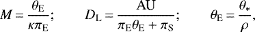 (1)
(1)
where κ = 4G∕(c2AU) and πS denotes the annual parallax of the source (Gould 2000). The value of the normalized source radius, ρ ~ 0.5 × 10⁻³, is firmly measured from the data points involved with caustic crossings at around t2 and t3. On the other hand, modeling that considers the microlens-parallax effect results in a πE value with aconsiderable uncertainty due to the fact that the photometry quality of the data is mediocre because of the faintness of the source, together with the fact that all the main features occur in an interval of 12 days, which is too short to appreciate any deviations due to parallax effects. Figure 9 shows the scatter plot of points in the MCMC chain on the πE,E–πE,N plane, where πE,E and πE,N are the east and north components of the microlens-parallax vector πE, respectively. The scatter plot shows that the microlens-parallax is consistent with a zero-parallax model within the 2σ level, and the uncertainty of πE,N is big, although the uncertainty of πE,E is relatively small. Considering that the anomaly features in the light curve occurred within a short time interval, the lens-orbital motion would not invoke any significant effects. Nevertheless, we conducted an additional modeling considering the lens-orbital model and found that the fit improvement by the lens-orbital effect is negligible and that the orbital motion was poorly constrained.
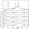 |
Fig. 3 Comparison of the four tested models, 1L2S, 2L1S, 2S2L, and 3L1S (close-close solution). The lower panels show the residuals from the individual models. |
Lensing parameters of the 1L2S, 2L1S, and 2L2S models.
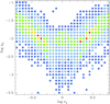 |
Fig. 4 Distribution of Δχ2 in the logs3– logq3 parameter plane obtained from the preliminary 3L1S grid searches for the parameters related to the third lens component. Red, yellow, green, cyan, and blue are used to denote points with Δχ2 < n(12), < n(22), < n(32), < n(42), and < n(52), respectively, where n = 10. |
Lensing parameters of four degenerate 3L1S models.
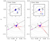 |
Fig. 5 Lens system configurations of the close-close (left panel) and close-wide (right panel) 3L1L models. The inset in each panel shows the locations of the three lens components, denoted by blue dots labeled M1, M2, and M3. The dashed circle in the inset represents the Einstein ring. The line with an arrow represents the source trajectory. The three small empty dots on the source trajectory represent the source positions at the epochs of t1, t2, and t3 that are marked in Fig. 1. The size of the dots is not scaled to the source size. The red figure represents the caustic, and the gray curves around the caustic represent equi-magnification contours. |
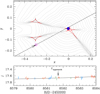 |
Fig. 6 Magnification pattern around the caustics (for the close-wide 3L1S model) and the light curve around the time of the source approach close to the planetary caustic induced by M2. The small empty circle on the source trajectory represents the source position at the time of the source approach, at tapproach ~ 8581.7 in HJD′. The size of the circle is arbitrarily set and is not scaled to the source size. |
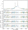 |
Fig. 7 Comparison of the residuals from the four degenerate 3L1S solutions: close-close, close-wide, wide-close, and wide-wide solutions. As a representative model, the model curve of the close-close solution is drawn over the data points in the top panel. |
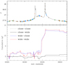 |
Fig. 8 Cumulative distributions of the Δχ2 difference from the best-fit solution (close-close model). The light curve in the upper panel is inserted to show the locations of the fit difference. |
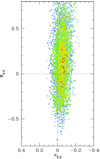 |
Fig. 9 Scatter plot of points in the MCMC chain on the πE,E–πE,N parameter plane for the close-close 3L1S solution. The color coding is the same as in Fig. 4, except n = 1. |
4 Source star and angular Einstein radius
For the determination of the angular Einstein radius, we needed to estimate the angular radius of the source. We deduced θ* from the color and brightness of the source. To estimate the extinction- and reddening-corrected (de-reddened) values,  , from the instrumental values, (V − I, I), we used the Yoo et al. (2004) method, in which the centroid of a red giant clump (RGC),
 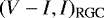 , in the color-magnitude diagram (CMD) is used for the calibration of the source color and magnitude.
Figure 10 shows the locations of the source (empty blue dot with error bars) and the RGC centroid (solid red dot) in the instrumental CMD constructed using the KMTC data processed using the pyDIA software (Albrow 2017). The source position in the CMD was determined via the regression of the I- and V -band pyDIA data with the variation of the lensing magnification. Also marked in the CMD is the blend position (solid green dot), which lies on the main-sequence branch of foreground disk stars. We show in Sect. 6 that the blended light is due to the host star, a companion to the host star, or a combination of the two. The measured instrumental color and brightness are (V − I, I) = (3.378 ± 0.099, 22.018 ± 0.004) for the source and  for the RGC centroid. By measuring the offsets in color, Δ(V − I), and magnitude, ΔI, between thesource and RGC centroid, together with the known de-reddened values of the RGC centroid,
  , from Bensby et al. (2013) and Nataf et al. (2013), respectively, we estimate that the de-reddened source color and magnitude are
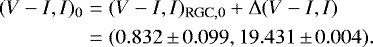 (2)
(2)
This indicates that the source is a late G-type main-sequence star located in the bulge.
For the θ* estimation from  , we first converted the measured V − I color into V − K color using the color-color relation of Bessell & Brett (1988) and second deduced the source radius from the (V − K)–θ* relation of Kervella et al. (2004). The estimated value is
 (3)
(3)
Together with the ρ and tE values measured from the modeling, the angular Einstein radius and the relative lens-source proper motion are estimated as
 (4)
(4)

respectively.
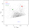 |
Fig. 10 Locations of the source (empty blue dot with error bars), RGC centroid (solid red dot), and blend (solid green dot) in the instrumental CMD of stars around the source constructed using the pyDIA photometry of the KMTC data set. |
5 Physical lens parameters
Although the mass and distance to the lens cannot be uniquely determined using the relation in Eq. (1) due to the insecure measurement of the microlens parallax, the physical parameters can still be constrained using the measured observables of tE and θE, which are related to M and DL by
 (6)
(6)
Here,  represents the relative lens-source parallax and DS denotes the distance to the source. For this constraint, we conducted a Bayesian analysis using a prior Galactic model. Although the uncertainty of the measured πE is big, we considered the measured πE by computing the parallax-ellipse covariance matrix in the Bayesian estimation of the physical lens parameters.
The Galactic model defines the physical and dynamical distributions and the mass function of Galactic objects. We adopted the Galacticmodel described in Jung et al. (2021). This model uses the Robin et al. (2003) and Han & Gould (2003) physical matter distributions to specify the locations of disk and bulge objects, respectively. It also uses the Han & Gould (1995) and Jung et al. (2021) dynamical distributions to describe the motions of disk and bulge objects, respectively. The mass function adopted in the model is described in Jung et al. (2018), and it includes stellar remnants and brown dwarfs.
In the first step of the Bayesian analysis, we conducted a Monte Carlo simulation to produce many (107) artificial lensing events, for which lens and source locations, transverse lens-source speeds, and lens masses are allocated following the Galactic model. Then, the microlensing observables (tE, θE, πE) of the individual events were computed using the relations in Eqs. (1) and (6). In the second step, we constructed the distributions of M and DL of events for which their observables are consistent with the observed values.
Figure 11 shows the posterior distributions of M and DL obtained from the Bayesian analysis. In Table 3, we list the estimated physical parameters of the masses of the individual lens components (M1, M2, M3), the distance, and the projected physical separations (a⊥,2, a⊥,3) between M1 –M2 and M1 –M3 pairs for the close-close and close-wide solutions. We adopted the median values of the distributions as representative parameters, and the uncertainties of the parameters were estimated as 16 and 84% of the distributions. The two solutions result in similar physical parameters, except for a⊥,3. The estimated mass of the host,
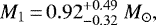 (7)
(7)
indicates that the host is a G-type star, and the distance,
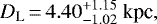 (8)
(8)
indicates that the lens is likely to be in the disk. The two planets have masses
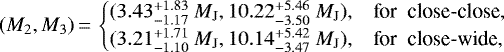 (9)
(9)
and thus both planets are heavier than Jupiter. Considering that the snow line distance from the host is dsl = 2.7(M∕M⊙) ~ 2.5 AU, the estimated separations,
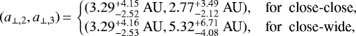 (10)
(10)
indicate that one planet lies near the snow line, and the other planet lies beyond the snow line.
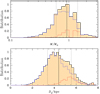 |
Fig. 11 Bayesian posterior distributions of the mass of (upper panel) and distance to (lower panel) the lens. In each panel, the solid vertical line indicates the median of the distribution, and the two dotted vertical lines indicate the 1σ range of the distribution. The blue and red curves represent the contributions by disk and bulge lenses, respectively. |
Physical lens parameters.
6 Baseline object
From the position of the blend on the CMD (Fig. 10), it is found that the flux of the baseline object is dominated by the light from a main-sequence star in the foreground disk. Logically, there are only four possibilities for this star: (1) the host of the planets, (2) a companion to the host, (3) a companion to the source, or (4) an ambient star that is unrelated to the event (or possibly a combination of two or more of these possibilities). The position of the blend on the CMD already rules out possibility (3) because it is inconsistent with a bulge star.
Because θE ~ 0.9 mas, the lens must also be in the foreground disk (unless it is a dark remnant). That is, if the lens were in the bulge, with πrel ≲0.02 mas, then its mass would be 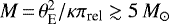 , implying that it would be easily seen. This suggests that the blended light may be due primarily to the host of the planets.
To test this conjecture, we first measured the astrometric offset between the “baseline object” and the source (which has the same position as the host at the time of the event). The position of the source is measured from difference images formed by subtracting the reference image from a series of images taken at high magnifications. This difference image essentially consists of an isolated star on a blank background. Hence, its position can be accurately measured. We find a scatter among 15 images of just (0.026, 0.037) pixels in the (east, north) directions, yielding a standard error of the mean of (0.007, 0.010) pixels, that is, (3, 4) mas, given the 400 mas pixel size. These errors are far below the other errors in the problem, which are discussed below. We therefore ignore them in what follows.
By contrast, the problem of measuring the position of the baseline object is far subtler. Its position is returned by the DoPhot photometry package (Schechter et al. 1993), which simultaneously fits for the positions and fluxes from possibly overlapping stellar images. Fortunately, the baseline object appears isolated in these images, so the statistical errors of this measurement are not strongly impacted by the algorithm’s procedure for separating stars. We estimated this error to be 23 mas in each direction from a comparison of two completely independent reductions, that is, by reductions determined by different people. We find the offset between the source and the baseline object to be
 (11)
(11)
If we could ignore systematic effects and take the error distributions to be a two-dimensional Gaussian, this would rule out the identification of the host with baseline light at p = 0.002 probability.
We note that this close alignment rules out possibility (4), that is, that the blended light is due to an ambient star. We simply counted the number of stars on the foreground main sequence in the 2 arcmin2 area of the OGLE finding chart that are brighter than the baseline object, finding N = 64. This translates to a surface density of n = 64∕1202 = 4.4 × 10⁻³ arcsec−2. Thus, the probability of such an alignment is  . Hence, the light from the baseline object must be due to either the planet host or a companion to the host (or a combination of the two).
Before considering these two remaining possibilities, we examined the role of the key systematic effect that could corrupt the position measurement of the baseline object at the ![$\Delta\theta\,{=}\, [\Delta\theta(N){}^2+ \Delta\theta(E){}^2]^{1/2}\sim 80$](/articles/aa/full_html/2022/02/aa42327-21/aa42327-21-eq21.png) mas level: namely, the possibility that an ambient star lies within the point-spread function of the baseline object. That is, if a fraction, f, of the blended light were due to an ambient star with a separation from the source of δθ, then the centroid of light (measured by DoPhot) would be displaced by Δθ = fδθ. For instance, for f = 0.2 and δθ = 400 mas, Δθ = 80 mas. In this example, the faint ambient starwith a separation of 0.4′′ would not be identified as a separate star by DoPhot, so the centroid would be shifted.
mas level: namely, the possibility that an ambient star lies within the point-spread function of the baseline object. That is, if a fraction, f, of the blended light were due to an ambient star with a separation from the source of δθ, then the centroid of light (measured by DoPhot) would be displaced by Δθ = fδθ. For instance, for f = 0.2 and δθ = 400 mas, Δθ = 80 mas. In this example, the faint ambient starwith a separation of 0.4′′ would not be identified as a separate star by DoPhot, so the centroid would be shifted.
We have just argued that ambient stars similar to or brighter than the baseline object are rare. However, ambient stars that could corrupt the astrometric measurement at this level are not rare, for three reasons. First, such stars are not restricted to the foreground main sequence, so the much larger population of bulge stars is available. Second, there are more faint stars than bright stars. Third, ambient stars can corrupt the astrometric measurement with separations of up to δθ ~ 1′′, whereas ambient stars that would explain the baseline object light must lie within Δθ = 80 mas. These three features also place limits on which ambient stars can play this role. First, if the ambient star were too bright (and came from the more populous, but redder, bulge population), then it would also drive the combined color of the resulting baseline object to the red, and so off the foreground main-sequence feature, contrary to its actual location. Second, if the ambient star were too faint, its separation would have to be δθ≳1′′, at which point its light would no longer enter into the DoPhot centroid. Third, as δθ is increased,ambient stars of sufficient brightness will be separately resolved by DoPhot before the δθ = 1′′ limit is reached.
To make our evaluation, we first focused our attention on the 2349 stars in the 2 arcmin2 OGLE-IV finding chart that satisfy 0.7 < (I − Ibase) < 2.7, where Ibase = 17.8 is evaluatedin the OGLE-IV system. The faint limit is set by the requirement δθ < 1′′, while the bright limit is set by the requirement that inclusion of the (usually) red ambient light does not drive the baseline object off the foreground main sequence. Then, for each of these 2349 stars we found the annulus of positions such that the star would induce an astrometric error of > 80 mas. The inner radius of the annulus is set by the flux ratio: δθinner = Δθ × 100.4(I−Ibase). We set δθouter = 0.2′′ [(I − Ibase) + 2.3]. We then find a total area subtended by these 2349 annuli to be 2800 arcsec2 (i.e., a fraction p = 19% of the 2 arcmin2) That is, if the host were primarily responsible for the blended light, then there is a p = 19% probability that an ambient star would corrupt the astrometric measurement by enough to account for the observed Δθ ~ 80 mas offset.
On the other hand, it is also possible that the baseline object has a fainter companion that generated the main microlensing event and so serves as the host for the planets. The main constraint on this scenario is that the blend, which is likely a G dwarf at several kiloparsecs, should have a widely separated companion at log (P∕day) ~ 4, with a mass ratio of qbase≳0.5. According to Table 7 of Duquennoy & Mayor (1991), about 25% of G dwarfs have companions with log (P∕day) > 4 and a mass ratio q ≥ 0.5. However, if the baseline object did have a companion in this parameter range, it is about equally likely that the baseline object served as the lens host for the event while the companion generated the flux required to corrupt the astrometric measurement.
In brief, there are two channels for the baseline object to be the host, with the astrometric measurement corrupted either by an ambient star (p = 0.19) or by a less luminous companion widely separated from the planet host (p = 0.25∕2 ~ 0.12) for a total of p = 0.31. By contrast, there is one channel for the host to be a companion of the baseline object, with probability p = 0.25∕2 ~ 0.12. Therefore, the host of the planet is likely responsible for the light of the baseline object, but the host could also plausibly be a companion to the baseline object. Considering the inconclusive nature of the blend together with the low quality of the spectra, we do not impose the constraint from the spectra on the estimation of the physical parameters presented in Table 3.
7 Summary and conclusion
We have reported a multiple planetary system discovered from the analysis of the lensing event OGLE-2019-BLG-0468, which was reinvestigated as part of a project of reviewing the microlensing data collected in and before the 2019 season by the KMTNet survey. The light curve of the event, which consists of three distinctive anomaly features, could not be explained by the usual 2L1S or 1L2S interpretations. We found a solution explaining all anomaly features with a 3L1S interpretation, in which the lens is composed of two planets and their host, making the lens the fourth multi-planet system securely found by microlensing. The lensing solution is subject to two-fold degeneracies caused by the ambiguity in estimating the separations of the planets from the host. One of the degeneracies is very severe, but the other was resolvable due to the resonant nature of the caustic induced by the second planet. The two planets have masses of ~ 3.4 MJ and ~ 10.2 MJ, and they are orbiting around a G-type star with a mass of ~0.9 M⊙ and a distance of ~4.4 kpc. It was found that the planet host was most likely responsible for the light of the baseline object, although the possibility of the host being acompanion to the baseline object could not be ruled out.
Acknowledgements
Work by C.H. was supported by the grants of National Research Foundation of Korea (2020R1A4A2002885 and 2019R1A2C2085965). S.D. acknowledges the science research grants from the China Manned Space Project with NO. CMS-CSST-2021-A11. This research has made use of the KMTNet system operated by the Korea Astronomy and Space Science Institute (KASI) and the data were obtained at three host sites of CTIO in Chile, SAAO in South Africa, and SSO in Australia. The observations using the SALT telescope were conducted under the transients follow up programme 2018-2-LSP-001 (PI: D.B.), which is supported by Poland under grant no. MNiSW DIR/WK/2016/07. D.B. also acknowledges research support from the National Research Foundation. M.G. is supported by the EU Horizon 2020 research and innovation programme under grant agreement No. 101004719.
References
- Albrow, M. 2017, https://doi.org/10.5281/zenodo.268049 [Google Scholar]
- Albrow, M., Horne, K., Bramich, D. M., et al. 2009, MNRAS, 397, 2099 [Google Scholar]
- Beaulieu, J.-P., Bennett, D. P., Batista, V., et al. 2016, ApJ, 824 [Google Scholar]
- Bennett, D. P., Rhie, S. H., Nikolaev, S., et al. 2010, ApJ, 713, 837 [Google Scholar]
- Bennett, D. P., Udalski, A., Han, C., et al. 2018, AJ, 155, 141 [Google Scholar]
- Bensby, T., Yee, J. C., Feltzing, S., et al. 2013, A&A, 549, A147 [NASA ADS] [CrossRef] [EDP Sciences] [Google Scholar]
- Bessell, M. S., & Brett, J. M. 1988, PASP, 100, 1134 [Google Scholar]
- Bozza, V. 1999, A&A, 348, 311 [NASA ADS] [Google Scholar]
- Buckley, D. A. H., Swart, G. P., & Meiring, J. G. 2006, SPIE Conf. Ser., 6267, 62670Z [Google Scholar]
- Burgh, E. B., Nordsieck, K. H., Kobulnicky, H. A., et al. 2003, SPIE, 4841, 1463 [Google Scholar]
- Chatterjee, S., Ford, E. B., Matsumura, S., et al. 2008, ApJ, 686, 580 [Google Scholar]
- Chung, S.-J., Han, C., Park, B.-G., et al. 2005, ApJ, 630, 535 [Google Scholar]
- Crawford, S. M., et al., 2010, Proc. SPIE, 7737, 773725 [NASA ADS] [CrossRef] [Google Scholar]
- Cumming, A., Butler, R. P., Marcy, G. W., et al. 2008, PASP, 120, 531 [CrossRef] [Google Scholar]
- Daněk, K., & Heyrovský, D. 2015a, ApJ, 806, 99 [CrossRef] [Google Scholar]
- Daněk, K., & Heyrovský, D. 2015b, ApJ, 806, 63 [CrossRef] [Google Scholar]
- Daněk, K., & Heyrovský, D. 2019, ApJ, 880, 72 [CrossRef] [Google Scholar]
- Dominik, M. 1999, A&A, 349, 108 [NASA ADS] [Google Scholar]
- Du, B., Luo, A.-L., Zuo, F., et al. 2019, ApJS, 240, 10 [NASA ADS] [CrossRef] [Google Scholar]
- Duquennoy, A., & Mayor, M. 1991, A&A, 248, 485 [NASA ADS] [Google Scholar]
- Fulton, B. J., Rosenthal, L. J., Hirsch, L. A., et al. 2021, ApJS, 255, 14 [NASA ADS] [CrossRef] [Google Scholar]
- Gaudi, B. S. 2012, ARA&A, 50, 411 [Google Scholar]
- Gaudi, B. S., Bennett, D. P., Udalski, A., et al. 2008, Science, 319, 927 [Google Scholar]
- Gould, A. 2000, ApJ, 542, 785 [NASA ADS] [CrossRef] [Google Scholar]
- Griest, K., & Safizadeh, N. 1998, ApJ, 500, 37 [Google Scholar]
- Han, C., & Gould, A. 1995, ApJ, 447, 53 [Google Scholar]
- Han, C., & Gould, A. 2003, ApJ, 592, 172 [Google Scholar]
- Han, C., Chang, H.-Y., An, J. H., & Chang, K. 2001, MNRAS, 328, 986 [NASA ADS] [CrossRef] [Google Scholar]
- Han, C., Udalski, A., Choi, J.-Y., et al. 2013, ApJ, 762, L28 [Google Scholar]
- Han, C., Bennett, D. P., Udalski, A., et al. 2019, AJ, 158, 114 [Google Scholar]
- Han, C., Kim, D., Jung, Y. K., et al. 2020a, AJ, 160, 17 [Google Scholar]
- Han, C., Kim, D., Udalski, A., et al. 2020b, AJ, 160, 64 [Google Scholar]
- Han, C., Lee, C.-U., Udalski, A., et al. 2020c, AJ, 159, 48 [Google Scholar]
- Han, C., Shin, I.-G., Jung, Y. K., et al. 2020d, A&A, 641, A105 [NASA ADS] [CrossRef] [EDP Sciences] [Google Scholar]
- Han, C., Udalski, A., Kim, D., et al. 2020e, A&A, 642, A110 [EDP Sciences] [Google Scholar]
- Han, C., Albrow, M. D., Chung, S.-J., et al. 2021a, A&A, 652, A145 [NASA ADS] [CrossRef] [EDP Sciences] [Google Scholar]
- Han, C., Lee, C.-U., Ryu, Y.-H., et al. 2021b, A&A, 649, A91 [NASA ADS] [CrossRef] [EDP Sciences] [Google Scholar]
- Han, C., Udalski, A., Kim, D., et al. 2021c, AJ, 161, 270 [NASA ADS] [CrossRef] [Google Scholar]
- Han, C., Udalski, A., Kim, D., et al. 2021d, A&A, 650, A89 [NASA ADS] [CrossRef] [EDP Sciences] [Google Scholar]
- Han, C., Udalski, A., Lee, C.-U., et al. 2021e, A&A, 649, A90 [EDP Sciences] [Google Scholar]
- Hwang, K.-H., Zang, W., Gould, et al. 2022, AJ, 163, 43 [NASA ADS] [CrossRef] [Google Scholar]
- Jung, Y. K., Udalski, A., Bond, I. A., et al. 2017, ApJ, 841, 75 [Google Scholar]
- Jung, Y. K., Udalski, A., Gould, A., et al. 2018, AJ, 155, 219 [Google Scholar]
- Jung, Y. K., Han, C., Udalski, A., et al. 2021, AJ, 161, 293 [NASA ADS] [CrossRef] [Google Scholar]
- Jurić, M., & Tremaine, S. 2008, ApJ, 686, 603 [Google Scholar]
- Kervella, P., Thévenin, F., Di Folco, E., & Ségransan, D. 2004, A&A, 426, 29 [Google Scholar]
- Kim, S.-L., Lee, C.-U., Park, B.-G., et al. 2016, JKAS, 49, 37 [Google Scholar]
- Madsen, S., & Zhu, W. 2019, ApJ, 878, L29 [NASA ADS] [CrossRef] [Google Scholar]
- Nataf, D. M., Gould, A., Fouqué, P., et al. 2013, ApJ, 769, 88 [Google Scholar]
- Robin, A. C., Reylé, C., Derriére, S., & Picaud, S. 2003, A&A, 409, 523 [NASA ADS] [CrossRef] [EDP Sciences] [Google Scholar]
- Rosenthal, L. J., Fulton, B. J., Hirsch, L. A., et al. 2021, ApJS, 255, 8 [NASA ADS] [CrossRef] [Google Scholar]
- Schechter, P. L., Mateo, M., & Saha, A. 1993, PASP, 105, 1342 [Google Scholar]
- Suzuki, D., Bennett, D. P., Udalski, A., et al. 2018, AJ, 155, 263 [Google Scholar]
- Udalski, A., Szymański, M. K., & Szymański, G. 2015, Acta Astron., 65, 1 [NASA ADS] [Google Scholar]
- Woźniak, P. R. 2000, Acta Astron., 50, 42 [Google Scholar]
- Wright, J. T., Upadhyay, S., Marcy, G. W., et al. 2009, ApJ, 693, 1084 [NASA ADS] [CrossRef] [Google Scholar]
- Yee, J. C., Shvartzvald, Y., Gal-Yam, A., et al. 2012, ApJ, 755, 102 [Google Scholar]
- Yoo, J., DePoy, D. L., Gal-Yam, A., et al. 2004, ApJ, 603, 139 [Google Scholar]
- Zang, W., Hwang, K.-H., Udalski, A., et al. 2021, AJ, 162, 163 [NASA ADS] [CrossRef] [Google Scholar]
- Zhu, W., & Dong, S. 2021, ARA&A, 59, 291 [NASA ADS] [CrossRef] [Google Scholar]
- Zhu, W., Penny, M., Mao, S., et al. 2014, ApJ, 788, 73 [Google Scholar]
All Tables
All Figures
|
Fig. 1 Light curve of the microlensing event OGLE-2019-BLG-0468. The arrows labeled t1 (8586.3), t2 (8592.9), and t3 (8595.7) indicate the three epochs of major anomalies. The curves drawn over the data points represent the 1L1S (dotted curve) and 3L1S (close-close model, solid curve) models. The zoomed-in view of the anomaly region around t2 and t3 is shown in Fig. 2. |
| In the text | |
|
Fig. 2 Zoomed-in view of the anomaly region around the epochs t2 and t3. Notations are the same as in Fig. 1. |
| In the text | |
|
Fig. 3 Comparison of the four tested models, 1L2S, 2L1S, 2S2L, and 3L1S (close-close solution). The lower panels show the residuals from the individual models. |
| In the text | |
|
Fig. 4 Distribution of Δχ2 in the logs3– logq3 parameter plane obtained from the preliminary 3L1S grid searches for the parameters related to the third lens component. Red, yellow, green, cyan, and blue are used to denote points with Δχ2 < n(12), < n(22), < n(32), < n(42), and < n(52), respectively, where n = 10. |
| In the text | |
|
Fig. 5 Lens system configurations of the close-close (left panel) and close-wide (right panel) 3L1L models. The inset in each panel shows the locations of the three lens components, denoted by blue dots labeled M1, M2, and M3. The dashed circle in the inset represents the Einstein ring. The line with an arrow represents the source trajectory. The three small empty dots on the source trajectory represent the source positions at the epochs of t1, t2, and t3 that are marked in Fig. 1. The size of the dots is not scaled to the source size. The red figure represents the caustic, and the gray curves around the caustic represent equi-magnification contours. |
| In the text | |
|
Fig. 6 Magnification pattern around the caustics (for the close-wide 3L1S model) and the light curve around the time of the source approach close to the planetary caustic induced by M2. The small empty circle on the source trajectory represents the source position at the time of the source approach, at tapproach ~ 8581.7 in HJD′. The size of the circle is arbitrarily set and is not scaled to the source size. |
| In the text | |
|
Fig. 7 Comparison of the residuals from the four degenerate 3L1S solutions: close-close, close-wide, wide-close, and wide-wide solutions. As a representative model, the model curve of the close-close solution is drawn over the data points in the top panel. |
| In the text | |
|
Fig. 8 Cumulative distributions of the Δχ2 difference from the best-fit solution (close-close model). The light curve in the upper panel is inserted to show the locations of the fit difference. |
| In the text | |
|
Fig. 9 Scatter plot of points in the MCMC chain on the πE,E–πE,N parameter plane for the close-close 3L1S solution. The color coding is the same as in Fig. 4, except n = 1. |
| In the text | |
|
Fig. 10 Locations of the source (empty blue dot with error bars), RGC centroid (solid red dot), and blend (solid green dot) in the instrumental CMD of stars around the source constructed using the pyDIA photometry of the KMTC data set. |
| In the text | |
|
Fig. 11 Bayesian posterior distributions of the mass of (upper panel) and distance to (lower panel) the lens. In each panel, the solid vertical line indicates the median of the distribution, and the two dotted vertical lines indicate the 1σ range of the distribution. The blue and red curves represent the contributions by disk and bulge lenses, respectively. |
| In the text | |
Current usage metrics show cumulative count of Article Views (full-text article views including HTML views, PDF and ePub downloads, according to the available data) and Abstracts Views on Vision4Press platform.
Data correspond to usage on the plateform after 2015. The current usage metrics is available 48-96 hours after online publication and is updated daily on week days.
Initial download of the metrics may take a while.