| Issue |
A&A
Volume 658, February 2022
|
|
|---|---|---|
| Article Number | A17 | |
| Number of page(s) | 20 | |
| Section | Interstellar and circumstellar matter | |
| DOI | https://doi.org/10.1051/0004-6361/202142233 | |
| Published online | 26 January 2022 | |
The ionised and molecular mass of post-common-envelope planetary nebulae
The missing mass problem★
1
Observatorio Astronómico Nacional (OAN-IGN),
Alfonso XII, 3,
28014
Madrid,
Spain
e-mail: This email address is being protected from spambots. You need JavaScript enabled to view it.
2
Instituto de Astrofísica de Canarias,
38205
La Laguna,
Spain
3
Departamento de Astrofísica, Universidad de La Laguna,
38206,
La Laguna,
Spain
4
Observatorio Astronómico Nacional (OAN-IGN),
Apartado 112,
28803
Alcalá de Henares,
Spain
5
Department of Physics and Astronomy, University College London,
Gower St,
London
WC1E 6BT,
UK
Received:
16
September
2021
Accepted:
28
October
2021
Abstract
Context. Most planetary nebulae (PNe) show beautiful, axisymmetric morphologies despite their progenitor stars being essentially spherical. Close binarity is widely invoked to help eject an axisymmetric nebula, after a brief phase of engulfment of the secondary within the envelope of the asymptotic giant branch (AGB) star, known as the common envelope (CE). The evolution of the AGB would thus be interrupted abruptly, with its still quite massive envelope being rapidly ejected to form the PN, which a priori would be more massive than the PN coming from a single version of the same star.
Aims. We aim to test this hypothesis by investigating the ionised and molecular masses of a sample consisting of 21 post-CE PNe, roughly one-fifth of the known total population of these objects, and to compare them to a large sample of ‘regular’ (i.e. not known to arise from close-binary systems) PNe.
Methods. We gathered data on the ionised and molecular content of our sample from the literature, and carried out molecular observations of several previously unobserved objects. We derived the ionised and molecular masses of the sample by means of a systematic approach, using tabulated, dereddened Hβ fluxes to find the ionised mass, and 12CO J = 2–1 and J = 3–2 observations to estimate the molecular mass.
Results. There is a general lack of molecular content in post-CE PNe. Our observations only reveal molecule-rich gas around NGC 6778, which is distributed into a low-mass, expanding equatorial ring lying beyond the ionised broken ring previously observed in this nebula. The only two other objects showing molecular content (from the literature) are NGC 2346 and NGC 7293. Once we derive the ionised and molecular masses, we find that post-CE PNe arising from single-degenerate (SD) systems are just as massive, on average, as members of the ‘regular’ PNe sample, whereas post-CE PNe arising from double-degenerate systems are considerably more massive, and show substantially higher linear momentum and kinetic energy than SD systems and ‘regular’ PNe. Reconstruction of the CE of four objects, for which a wealth of data on the nebulae and complete orbital parameters are available, further suggests that the mass of SD nebulae actually amounts to a very small fraction of the envelope of their progenitor stars. This leads to the uncomfortable questions of where the rest of the envelope is and why we cannot detect it in the stars’ vicinity, raising serious doubts about our understanding of these intriguing objects.
Key words: planetary nebulae: general / planetary nebulae: individual: NGC 6778 / circumstellar matter / binaries: close / stars: mass-loss / stars: winds, outflows
Reduced data are only available at the CDS via anonymous ftp to cdsarc.u-strasbg.fr (130.79.128.5) or via http://cdsarc.u-strasbg.fr/viz-bin/cat/J/A+A/658/A17
© ESO 2022
1 Introduction
Low- and intermediate-mass (up to ~8 M⊙) stars end their lives by ejecting their envelope into beautiful nebulae with intricate geometries. The resulting planetary nebulae (PNe) show high degrees of symmetry, with mostly bipolar or elliptical morphologies. The mechanism behind the shaping of axisymmetric PNe has been a matter of debate for the last few decades (e.g. Balick & Frank 2002), although it is becoming increasingly clear that angular momentum from a binary or substellar companion is a key ingredient to this intriguing puzzle (Jones & Boffin 2017; Decin et al. 2020).
The close binary central stars of PNe (CSPNe) are evolved binaries with orbital separations that are orders of magnitude smaller than the typical radius of an asymptotic giant branch (AGB) star. As such, the component stars must have previously interacted and evolved to this separation rather than having formed at such proximity. The mechanism, first proposed by Paczynski (1976), by which these systems reach their current configuration is thought to proceed in the following manner: as the primary star evolves along the giant branch(es) and expands, copiously losing mass through a slow wind, it eventually expands to overflow its Roche lobe. Runaway mass transfer on to the secondary then occurs through the inner Lagrangian point on dynamical timescales, engulfing the companion and leading to the formation of a common envelope (CE). In this brief (~1 yr) phase, the secondary quickly spirals inwards inside the extended envelope of the primary due to drag forces, leading to either a merging of the two stars or the abrupt end and ejection of the CE (Ivanova et al. 2013). In the latter case, the envelope is shaped into a bipolar planetary nebula whose equator would coincide with the system’s orbital plane. This is indeed the case in every one of the eight cases analysed so far, in which the orientation of the orbital plane and nebula equator could be determined (Hillwig et al. 2016; Munday et al. 2020). Such a correlation constitutes the strongest statistical proof so far of the influence of close binarity in the shaping of PNe.
The first observational confirmation of the existence of PNe with close-binary nuclei was obtained by Bond (1976) in Abell 63. A few other cases came in the following years, although the hypothesis did not really gain popularity until the arrival of modern, systematic photometric surveys such as the Optical Gravitational Lensing Experiment (OGLE; Udalski et al. 2008), when dozens of close-binary central stars of PNe were detected and a solid lower limit of ≳ 15% was established for the post-CE binary fraction (Miszalski et al. 2009). The identification of morphological traits such as rings, jets, and fast, low-ionisation emitting regions as characteristic trends indicative of close binarity further enhanced the statistics (e.g. Miszalski et al. 2011a,b; 2012, Jones et al. 2014, 2015; Corradi et al. 2011; Santander-García et al. 2015b) up until the present number of approximately 100 confirmed binary CSPNe1.
However, on theoretical grounds, a deeper understanding of the physics of the CE remains very elusive (Ivanova et al. 2013; Jones 2020). Most hydrodynamic models are unable to gravitationally unbind the whole envelope, effectively ejecting no more than a few tenths of the whole envelope (Ohlmann et al. 2016; Ricker & Taam 2012; García-Segura et al. 2018), either because they lack key physical ingredients or because of fundamental hardware limitations (see Chamandy et al. 2020). Exceptions require resorting to additional energy reservoirs, such as the recombination energy from the ionised region, which is debated (Webbink 2008; Ricker & Taam 2012; Nandez et al. 2015; Ivanova 2018; Sand et al. 2020). In summary, although simulations collectively show that the CE has a major role in shaping PNe, we arefar from fully understanding the physics behind the death of a significant fraction of stars in the Universe.
Careful estimation of the mass of these envelopes could provide insight into CE ejection through constraints that can then be fed back into modelling efforts. We can in principle derive this parameter by determining the total masses of the resultant PNe under the assumption of sudden ejection of the CE into forming the PNe, i.e. assuming the mass of the CE mass is equal to the mass of the PN – excluding any halo, which would have been deployed into the interstellar medium (ISM) long before the CE stage. In this respect, it will also be useful to put these mass figures in the context of the general population of PNe, encompassing nebulae arising not only from close binaries but also from single stars and longer period binary stars that did not experience aCE.
It can be argued that CE evolution implies significant differences in the mass-loss history of the central star with respect to single star evolution. Let us consider a single AGB star first. Most of the mass lost by such a star along its evolution via slow winds gets too diluted in the ISM to be detected later during the PN stage (McCullough et al. 2001; Villaver et al. 2002). It is instead the mass lost during the superwind phase (lasting ~500–3000 yr) that will conform the PN, amounting to ~0.1–0.6 M⊙ for a star with an initial mass of 1.5 M⊙ (see review in Höfner & Olofsson 2018). Should the same AGB star be part of a close-enough binary system, its evolution will be abruptly interrupted as soon as it expands to fill its Roche-lobe, engulf its companion, and undergo the CE stage. This can be expected to occur in the final few (~1–20) million years of the AGB stage (e.g. Fig. 3 in Jones 2020). Thus, upon ejection of the CE, the resultant PN should in principle comprise all the mass the AGB star did not deploy into the ISM during these last million years (cf. only the last few thousand years for the single-star scenario outlined above). Due to the premature, sudden ejection of the CE, no massive extended haloes are expected in the near vicinity of this expanding PN. Therefore, one would expect PNe arising from a CE to be more massive on average than their single-star and long-period binary counterparts2.
Nevertheless, the only mass determinations of post-CE PNe available in the literature appear to support the opposite idea. Frew & Parker (2007) calculated the ionised masses of a sample of post-CE PNe and found them to be lower, on average, than those of the general PNe population (a finding later reinforced by Corradi et al. 2015). However, Frew & Parker (2007) and Corradi et al. (2015) only included the ionised mass in their calculations, not accounting for the potential presence of material not yet ionised or photo-dissociated by the UV radiation from the white dwarf (WD). Recent work on the dust emission around post-red-giant-branch (post-RGB) stars in the LMC, which are thought to have undergone a CE which cut short their evolution, indicates that the dust mass in these objects is similarly very low (10−7–10−4 M⊙) indicating that the ‘missing mass’ is not hiding in a dusty disk or shell (Sarkar & Sahai 2021). However, little is known about the molecular or neutral gas content of post-CE PNe.
With the goal of reaching a better understanding of this issue, in this work we derive the ionised and molecular mass of a sample of 21 post-CE PNe, representing roughly 20% of the total known objects of this kind. The paper is organised as follows: in Sect. 2 we present the sample and describe the molecular line observations and data reduction. Section 3 deals with the millimetre(mm)-wavelength emission detected in our observations, and its modelling. We calculate the ionised and molecular mass of the whole sample, and compare it to regular PNe (i.e. PNe not confirmed to host a close binary) in Sect. 4. Finally, we discuss the results in Sect. 5 and summarise our conclusions in Sect. 6.
2 Sample and observations
The sample of post-CE PNe analysed in this work consists of two subsamples. The first one consists of nine northern post-CE PNe previously unobserved in 12CO and 13CO J = 1–0 and J = 2–1, observations of which were secured with the IRAM 30m radio telescope (see the top part of Tables 1 and 2 for details). These nebulae are relatively compact so as to fit inside the telescope beam in one or a few pointings, in order to account for their whole CO content as accurately as possible. This subsample was selected to cover a broad range of kinematical ages, orbital periods, and morphologies. All of them show some emission excess in the far-infrared (IR), with bumps peaking at 25–60 μm, which in evolved stars (still not undergoing ionisation) correlates with CO emission (see e.g. Bujarrabal et al. 1992). Observations were carried out in two runs, in December 2017 and May 2018. The telescope half power beam width (HPBW) was 10.7 and 21.3 arcsec at 230 GHz and 110 GHz, respectively, according to the latest telescope parameters provided by IRAM. The FTS200 backends were used, and the spectral resolution degraded to 1 km s−1 in order to better detect the molecular profiles of these PNe, which are expected to be in the range of 20–80 km s−1 in width. Datawere reduced using standard baseline-subtraction and averaging procedures in the Continuum and Line Analysis Single-dish Software (CLASS) software, part of the GILDAS suite3, and flux-calibrated in the main-beam (Tmb) scale. Only one PN in this subsample, NGC 6778, was detected in these observations (12CO J = 1–0 and J = 2–1, 13CO J = 2–1). See Fig. 1 for the detected mm-wavelength emission, and Sect. 3 below for an analysis of the molecular emission in this nebula.
A second subsample was constructed from every molecular observation of PNe now confirmed to host a post-CE binary found throughout the literature (Huggins & Healy 1989; Huggins et al. 1996, 2005; Guzman-Ramirez et al. 2018 and references therein). These comprise another 12 post-CE PNe observed with the NRAO 12m, APEX 12m, SEST 15m, or IRAM 30m radio telescopes, in different configurations including 12CO J = 1–0 and/or J = 2–1 or J = 3–2. The only exclusion in this work is that of HaTr 4, observed (and undetected) by Guzman-Ramirez et al. (2018), because no integrated, dereddened Hβ (or Hα) flux could be found in the literature. The bottom part of Tables 1 and 2 summarises these observations, providing the transitions used, the velocity resolution, the rms achieved around the undetected line, or the integrated flux, depending on the case. These figures were extracted directly from Huggins & Healy (1989) and Huggins et al. (1996), while data from Guzman-Ramirez et al. (2018) were reanalysed from APEX archival data, because these authors did not provide the velocity resolution corresponding to their quoted sensitivities. The resulting data of this subsample follow a similar pattern to our own observations: only two objects, NGC 2346 and NGC 7293, show molecular emission down to the different sensitivities achieved.
Post-CE PNe undetected at mm wavelengths.
Post-CE PNe detected at mm wavelengths.
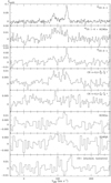 |
Fig. 1 Detected (and tentatively detected) mm-wavelength emission at the position of the central star of NGC 6778. The systemic VLSR is 107.1 km s−1. An asterisk indicates that the velocity of the CN line complexes shown, with J = 3∕2–1/2 and J = 1∕2–1/2, are referenced to frequencies of 113.490985 GHz and 113.157347 GHz, respectively. The tentative CO+ line shown is a stack from the N = 2–1 group with J = 3∕2–3/2, 3/2–1/2, and 5/2–3/2. |
3 Millimetre wavelength emission from NGC 6778
The only detection in our observations with the IRAM 30m telescope was that of NGC 6778. The flux-calibrated (Tmb scale) profiles of detected transitions at the position of the central star system are displayed in Fig. 1. Observations are compatible with a systemic VLSR of 107.1 km s−1.
In addition to 12CO and 13CO, we detected CNv = 0 J = 3∕2–1/2 and the J = 1∕2–1/2 system, as well as the hydrogen recombination lines H(30)α and H(48)β. These lines are displayed in Fig. 1, while their integrated intensities are shown in Table 2. CO+ (N = 2–1) is also tentatively detected, with its most prominent component peaking at a velocity of ~+13 km s−1 redward of the systemic velocity, which is considerably faster than the peaks seen in 12CO, but still below the ~26 km s−1 velocity displayed by the material in the optical range (Guerrero & Miranda 2012), which would suggest the existence of a region between the molecule-rich and the ion-rich regions, where CO could be ionised by UV photons from the central star, should the tentative detection of CO+ be confirmed in this source.
3.1 12CO and 13CO in NGC 6778
The 12CO J = 1–0 profile is contaminated by close H(38)α emission at 115274.41 MHz. In order to account for this contamination, we computed the relative fluxes of different hydrogen recombination lines in IRAM 30m survey spectra of one of the best-studied PNe, NGC 7027. Assuming similar physical conditions for the ionised component of NGC 6778, we concluded the intensity of H(38)α to be 0.65 times that of the detected H(30)α line (see Fig. 1) at 231900.928 MHz. We therefore used a scaled-down H(30)α profile as a template for subtracting the H(38)α from the 12CO J = 1–0 spectral profile, resulting in the middle panel of Fig. 2.
The detected 12CO and 13CO spectral profiles are double-peaked, with peak velocities similar to (although slightly lower than) those found by Guerrero & Miranda (2012) in the [N II]-emitting equatorial, distorted ring. The CO-rich domain of this nebula seems to be constrained to the central region judging from the substantial emission decrease when offsetting the telescope by10 arcsec along the equatorial direction, and the sharp drop at positions 12.5 and 14 arcsec away along the nebular axis (see Fig. 3). With respect to peak intensities, the blue peak is fainter both in 12CO and 13CO. More specifically, the peak-to-peak ratio is larger in 13CO than it is in 12CO, thus ruling out self-absorption, and pointing towards a clumpy, inhomogeneous matter distribution.
We therefore interpret this structure as a thin equatorial ring with an approximate projected size of 14 × 7.5 arcsec2 (and thus an inclination of ~32° to the line of sight), which we use for computing the molecular mass in Sect. 4. We built a spatio-kinematical model including radiative transfer in CO lines under the Large Velocity Gradient (LVG) assumption, by making use of the SHAPE+shapemol code (Steffen et al. 2011; Santander-García et al. 2015a). Given the limited amount of geometric information available and the blueward and redward peak differences, for the sake of simplicity the model is split into two semi-tori receding from and approaching the observer, respectively.
The achieved best-fit is shown in red in Figs. 2 and 3, and the corresponding parameters, along with uncertainties (as estimated by varying each individual parameter until a fair fit is no longer achieved) are provided in Table 3. The characteristic microturbulence velocities of the receding and approaching structures were found to be of 3 and 4 km s−1, respectively.
We found the 12CO to 13CO abundance ratio to be as low as four, although typical calibration errors ranging from 10% to 20% would allow for somewhat larger abundance ratios. In any case, it is worth noting that such a low isotopic ratio could indicate an O-rich nature for this source (e.g. Milam et al. 2009).
The density, volume, and 12CO abundance found for this structure allows for a molecular mass estimate independent from the method followed in Sect. 4. With theassumption that the bulk of the mass consists of hydrogen molecules, and an additional correction factor of 1.2 to account for helium abundance (assumed to be H/He = 0.1), the resulting molecular mass of NGC 6778 is 1.1 × 10⁻² M⊙. This figure is compatible within errors with the molecular mass found in Sect. 4 for this object, namely 0.024 ± 0.02 M⊙. We note that, given the apparent clumpy nature of this equatorial ring, the actual mass could be somewhat higher due to opacity being higherthan modelled in this section.
Best-fit model parameters for the molecular component of NGC 6778.
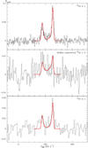 |
Fig. 2 Detected 12CO and 13CO emission profiles at the position of the central star system of NGC 6778 (black), and corresponding SHAPE+SHAPEMOL model synthetic emission profiles (red). A Gaussian profile simulating H(38)α has been subtracted from the 12CO J = 1–0 emission in order to account for contamination from this recombination line (see text). |
3.2 CN in NGC 6778
We modelled the detected CN emission using the hyperfine-structure-dedicated CLASS method. The result is displayed in Fig. 4. The resulting optical depth of the main component is 0.7 ± 0.4. Alternatively, the proportion existing between the intensities and integrated areas of the J =3∕2–1/2 and J =1∕2–1/2 groups suggests that the CN lines are relatively optically thin, and therefore that the excitation temperature is probably relatively low.
We further investigated the abundance of CN by means of simple modelling. Assuming LTE conditions and that the spatial distribution of CN is similar to that of CO, we can compare column densities resulting from simple LTE modelling of the nearby 12CO J = 1–0 and 13CO J = 2–1, both of which we assume to be optically thin and at a temperature of 50 K, as found in Sect. 3.1. We consider two models for CN, with temperatures of 10 K and 50 K, respectively. Using the 12CO and 13CO abundances found in Sect. 3.1, we arrive at a range of CN abundances XCN of between 3 × 10⁻⁷ and 8 × 10⁻⁷ when comparing with 12CO J = 1–0, and between 3 × 10⁻⁷ and 1 × 10⁻⁶ when comparing with 13CO J = 2–1. Despite the obvious lack of information on the CN emission properties, our CN relative abundance estimates are remarkably coherent. The relatively high abundance deduced for NGC 6778 is within the range of values found in PNe (e.g. Bachiller et al. 1997a,b), somewhat higher than abundances in O-rich AGB stars but lower than in C-rich AGBs. This probably reflects the somewhat rich chemistry existing in a photodissociation region (PDR), something characteristic of PNe rather than of circumstellar envelopes of giant stars.
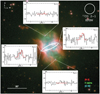 |
Fig. 3 Equatorial ring model (white) of the 12CO and 13CO emission of NGC 6778 overlaid on an image of the nebula taken with the NOT telescope (adapted from Guerrero & Miranda 2012). White crosses mark the observed offset positions, while associated insets show their corresponding 12CO J = 2–1 emission profiles (black) and SHAPE+SHAPEMOL model synthetic profiles (red). The HPBW of the IRAM 30m telescope at the 12CO J = 2–1 transition is indicated by the white circle. |
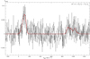 |
Fig. 4 CN v = 0 J = 3∕2–1/2 and J = 1∕2–1/2 line complexes in NGC 6778. The red line indicates hyperfine structure modelling of CN emission (see Sect. 3.2). |
4 The mass of post-CE PNe
We derived the ionised and molecular masses of the sample of post-CE PNe in a systematic manner in order to find patterns and correlations that can inform models of the CE. In this section, we describe the analyses performed on both ionised and molecular components, discuss their scope and limitations, present our results, and provide some context by comparing them to the masses of a large sample of PNe derived in the same fashion.
4.1 Ionised masses
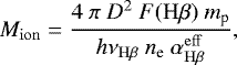
The total ionised masses of the PNe in the sample were calculated using the relation:
 (1)
(1)
where D is the distance, F(Hβ) is the dereddened, spatially integrated Hβ flux, mp is the mass of the proton, hνHβ is the energy of an Hβ photon, ne is the electron density, and  is the effective recombination coefficient of Hβ (Corradi et al. 2015).
In order for results to be as standardised as possible, we almost exclusively used F(Hβ) fluxes derived from the dereddened S(Hα) surface brightness tabulated by Frew et al. (2016), integrated over the ellipse defined by the minor and major axes tabulated by the same authors. We also used T[O III] determinations for the electron temperatures, except in those cases without available data, where we assumed Te = 10 000 K. As for electron densities, we almost exclusively used determinations based on the [S II] line doublet, except in the case of NGC 246, where only an estimate based on [O II] was available. Finally, with respect to the distances to the objects, we prioritised Gaia eDR3 determinations by Gaia Collaboration (2021) as long as they both matched identifications by Chornay & Walton (2020, 2021), and their associated errors were < 33%. In the absence of these, we used distances by Frew et al. (2016), or distance determinations to particular objects available in the literature, should the former also be absent. Every parameter used in this analysis, along with its reference, is shown in Table B.1.
In each case, the ionised mass and corresponding uncertainty was derived using 100 000 Monte Carlo samples of the distance, electron temperature, electron density, and Hβ flux. A normal probability distribution was used for distances quoted with symmetric uncertainties, while for distances with asymmetric uncertainties the probability distribution was assumed to be log-normal. Where no uncertainty was available, a normal distribution was employed corresponding to an uncertainty of ± 20%. For electrontemperature, again a normal distribution was employed and with an uncertainty of ±5% assumed in cases where no uncertainty was available in the literature. For the electron density, a log-normal probability distribution was assumed as this was found to be the best representation of the distribution based on a random sampling of a Gaussian distribution for the underlying emission line ratio, [S II]λλ 6716 Å/6732 Å (Wesson et al. 2012). Where no uncertainty on the density was available, an uncertainty on the emission line ratio of 0.2 was assumed and propagated through to the derived density uncertainty. The effective recombination coefficient of Hβ was calculated using the relationship of Storey & Hummer (1995), taking into account the dependence on both electron density and temperature.
4.2 Molecular masses
Only three objects in our sample show molecular emission in either our observations (NGC 6778, see Sect. 3) or the data available in the literature (NGC 7293, Huggins & Healy 1986; NGC 2346, Huggins et al. 1996). We therefore derived the molecular mass for these three objects, as well as conservative (3-σ) upper limits to the molecular mass of the rest of the sample based on the sensitivities achieved.
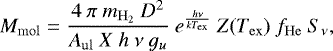
The method for estimating the molecular mass of these PNe from their CO emission relies on several simple assumptions: (i) the CO level populations are in local thermodynamic equilibrium (LTE), and thus they can be characterised by a single excitation temperature Tex ; (ii) the CO abundance X relative to hydrogen is constant throughout the molecule-rich nebula; and (iii) the selected CO transition is optically thin. Conditions (i) and (ii) are very probably satisfied in molecule-rich components, because of the favourable excitation and chemical conditions of CO (see e.g. Huggins et al. 1996; Bujarrabal et al. 2001). Condition (iii) is discussed below. These three conditions being fulfilled, the total molecular mass Mmol of a nebula is:
 (2)
(2)
where  is the mass of the hydrogen molecule, h and k are the Planck and Boltzmann constants respectively, ν is the frequency of the transition, Aul its Einstein coefficient, gu the degeneracy of its upper state, Z the partition function, D the distance to the nebula, fHe the correction factor to account for helium abundance (assumed to be He/H = 0.1 and thus resulting in fHe = 1.2, because we also assume the majority of particles to be of molecular hydrogen), and Sν the flux density of the transition, which in turn is:
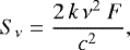 (3)
(3)
where c is the speed of light in vacuum, and F the total flux of the nebula in the given transition, integrated both spatially and spectrally. We computed the molecular masses of our sample following this scheme, assuming an excitation temperature of Tex = 50 K, and a CO abundance X = 2 × 10⁻⁴ for every object. The majority of the data for the CO emission from our sample (as well as in general for PNe) available in the literature are from surveys of 12CO J = 2–1, and sometimes of the weaker 12CO J = 1–0 at fairly low sensitivities, such as those by Huggins & Healy (1989), and Huggins et al. (1996, 2005). Data for a few objects come instead from a survey of 12CO J = 3–2 emission (Guzman-Ramirez et al. 2018).
It has been noted that both the 12CO J = 2–1 and J = 3–2 lines are often optically thick to some degree in PNe, thus resulting in the underestimation of molecular masses in those studies. While 13CO J = 1–0 and J = 2–1 emission is generally optically thin in PNe, and thus would warrant accurate mass determinations, their detection is much more difficult given their relatively low intensities, and hence data from these lines are very scarce in the literature.
In order to overcome this limitation and provide systematic, statistically meaningful, yet simple estimates ofmolecular masses of the sample of post-CE PNe, we opted for the following approach. Our observations of NGC 6778 plus a literature search reveal seven PNe with detected emission of both 12CO J = 1–0 and J = 2–1, and six more with detected emission of both 12CO J = 2–1 and J = 3–2 (Huggins et al. 1996, 2005; Guzman-Ramirez et al. 2018). We therefore computed their masses according to each of the transitions, and computed the average correction factor needed to correct the underestimated masses resulting from J = 2–1 and J = 3–2 transitions in order to match masses found via the J = 1–0 transition. These resulted in a factor 3.65 to be applied to calculations using 12CO J = 2–1 and a factor 5.0 for those using 12CO J = 3–2. We therefore apply these correction factors to every PN of the sample in our molecular mass estimates. Although the validity of these correction factors will vary from object to object, depending on its particular physical conditions (as other assumed values, such as the excitation temperature and CO abundance, indeed do), such a systematic correction allows for statistical comparisons with the ionised mass of these objects, and among subclasses of post-CE PNe.
In the two cases where 12CO emission is detected and mapping measurements are available (NGC 2346 and NGC 7293), we used those as the flux value F. In the case of NGC 6778, we estimated the flux by assuming constant surface brightness over the whole nebula. Thus, we integrated the detected intensity over an ellipse with major axes as estimated in Sect. 3, coupled with the telescope beam. For the rest the sample, we used the 3-σ sensitivities achieved to infer an upper limit to the intensity I. In order to derive the corresponding flux F, we integrated I spatially over the ellipse defined by the nebular major and minor axes tabulated by Frew et al. (2016) and coupled with the telescope beam, and spectrally over an assumed velocity width of 45 km s−1 wherever the telescope beam was larger than the nebular average diameter, and of 45 km s−1 (down to a minimum of 3 km s−1) wherever the beam was smaller than the nebula (with its diameter defined as the mean of its axes), thus following the same strategy as Huggins et al. (1996). We note that this approach is unlikely to underestimate the molecular mass of the nebulae, because the coupling of the telescope beam with an ellipse of constant surface brightness and size as large as the optical nebula systematically results in a larger flux than that resulting from single-dish mapping, that is, for the 13 out of 15 nebula in which both measurements are available (Huggins et al. 1996), with these excesses having a geometric mean of 2.4. Finally, for the criteria followed for selecting the distances to the objects, see Sect. 4.1.
Calculated errors correspond to formal error propagation. Parameters including formal errors are the distance, the correction factors discussed above (for which we take their standard deviation as error), and a 20% relative error in intensities and fluxes to account for telescope calibration uncertainties. Every parameter used in our analysis is displayed in Table B.1
Computed ionised and molecular masses of the post-CE sample.
4.3 Results
The ionised and molecular masses found in this work for the analysed sample of post-PNe are shown in Table 4. An interesting trend arises when dividing the sample into two categories, namely single-degenerate (SD) and double-degenerate (DD) systems, according to one or both components of the binary pair being a post-AGB star, respectively. Thus, PNe hosting DD systems seem substantially more massive than those hosting SD systems. The ionised and molecular masses of the whole sample are displayed in Fig. 5.
We note that the analysis presented here does not take into account any mass that could be present in neutral, atomic form, located in a photo-dissociation region (PDR) between the inner ion-rich region, and the outer, molecule-rich one. The reason for this is the lack of observations of spectral features suitable for determining low-excitation, neutral masses; for example the [C II] 158 μm line, which is unobservable with ground-based telescopes (see e.g. Castro-Carrizo et al. 2001; Fong et al. 2001). Indeed, to our knowledge, the only existing observations of post-CE PNe at this wavelength are unpublished data of NGC 2392 by HERSCHEL/HIFI + PACS, which allow us to estimate that the neutral mass of this nebula amounts to a mere 2 × 10⁻³ M⊙ (Santander-García et al., in prep.). This is in line with the derived values of the neutral atomic mass in other studied PNe, which is almost always ≲0.1 M⊙ (Castro-Carrizo et al. 2001; Fong et al. 2001). This, together with the lack of molecular emission from most post-CE SDPNe and every DD PNe in the sample, hints at the possibility that the gas surrounding these systems tends to be fully ionised. The neutral mass of these systems is unlikely to be substantial enough to change the findings of this paper, although it certainly merits being the focus of future work (Santander-García et al., in prep.).
Figure 6 shows the mass distribution of each subclass, where a given nebula falls inside a mass bin according toits ionised + molecular mass, or, in the absence of the latter, the sum of its ionised mass and the upper limit to its molecular mass. Hence, the mass distribution plotted there provides a conservative idea of the total ionised + molecular mass that the post-CE PNe may have. Even though they fall in the same range, it appears from Fig. 6 and Table 4 that PNe surrounding DD systems tend to be more massive than those around SD binaries. In fact, the geometric mean of the (thus-defined) ionised+molecular mass for the SD sample is 0.15 M⊙, with a geometric standard deviation (GSD) factor of 3.4, whereas for the DD sample the geometric mean is substantially larger, 0.31 M⊙, with a narrower GSD of 1.7.
We can also make an educated guess about the linear momentum and kinetic energy displayed by these objects (again, neglecting any neutral mass that may be present, and treating upper limits to the molecular mass as the molecular mass itself). To this respect, we used characteristic expansion velocities found throughout the literature (prioritising systematic works such as that by Weinberger 1989 which take the velocity of the nebula close to the central star and along the line of sight as the characteristic expansion velocity). These can be found in Table B.1 alongside the parameters used in this paper. We were able to find expansion velocities for every object of the sample except for four SD systems. These seem to follow a similar trend to ionised + molecular mass, being somewhat larger in DD systems than in SD ones.
The resulting linear momenta have substantially different geometric means of 6.3 × 1038 g cm s−1 (with GSD factor 3.5) and 2.2 × 1039 g cm s−1 (with GSD factor 2.3), for SD and DD systems respectively. As for the kinetic energy of the outflows, their geometric means differ in an even more pronounced way, being 8.1 × 1044 erg (with GSD factor 3.7) for SD systems, and 3.9 × 1045 erg (with GSD factor 4.2) for DD ones. In summary, it seems that both the mass and the velocity (and therefore the linear momentum, and particularly the kinetic energy) of DD post-CE PNe are higher, in general, than those of their SD counterparts.
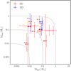 |
Fig. 5 Ionised vs. molecular mass of our post-CE PNe sample. The further to the top and to the right a nebula is, the more massive it is. Dashed lines represent ‘isomasses’, indicating equal ionised + molecular mass; neglecting neutral atomic mass (see Sect. 4.3), individual nebulae run along these lines as their gas content is progressively ionised. |
4.4 Comparison with regular PNe
In this section, we try to put previous findings in the context of the general population of PNe. Are post-CE PNe more massive on average than the general population of PNe, as hypothesised in Sect. 1? The answer to this question, as elusive as it may be, may have strong implications for theories of formation of PNe via CE interaction.
In order to bring some insight into this topic, we built an additional, larger sample consisting of ‘regular’ PNe, that is, PNe showing no evidence of hosting a close-binary system. We note that this may include both genuine single-star PNe and PNe hosting still undetected post-CE binaries or mergers. A PN had to fulfill the following criteria in order to be included in the regular sample: (i) being listed in Frew et al. (2016), thus having available a dereddened Hα flux and diameters obtained in a systematic way; (ii) having available 12CO observations (whether detected or not) to allow its molecular mass (or upper limit to it) to be accounted for; (iii) having an accurate distance determination, that is, a Gaia eDR3 measurement as identified by Chornay & Walton (2020, 2021) with an associated error < 33% or, lacking those, being listed as ‘distance calibrator’ by Frew et al. (2016) in their Table 3; and (iv) having an available determination of its characteristic electronic density ne (based on the [S II] doublet wherever possible).
We therefore built a sample consisting of 97 PNe, essentially by cross-matching the catalogue by Frew et al. (2016) with the molecular surveys by Huggins & Healy (1989); Huggins et al. (1996, 2005), and Guzman-Ramirez et al. (2018), rejecting those PNe whose distance was not accurate enough, or for which there was no available measurement of their ne. We prioritised Te determinations based on [O III] where possible, and assumed a Te = 10 000 K wherever no temperature determination was available in a literature search. The only exceptions to this approach are those of NGC 6302, NGC 7027, and NGC 7354, for which we used He-corrected molecular masses found by Santander-García et al. (2017, 2012), and Verbena et al. (in prep.), respectively. We highlight that NGC 6302 is the only case in the whole sample analysed in this work whose molecular data include interferometric measurements subject to flux loss, but we include it nevertheless, because the analysis by Santander-García et al. (2017) found the same mass as in the previous analysis by Santander-García et al. (2012), which included several singled-dish HERSCHEL/HIFI transitions at frequencies at which the telescope beam FWHM was as large as 20 arcsec, and found interferometric flux loss to be moderate. The sample is listed in Table B.1 along with every parameter used in this study.
We note that such a sample is not limited by volume and is thus not exempt from selection biases. Whereas Huggins & Healy (1989) and Huggins et al. (1996) selected their sample to include objects thought to be at distances shorter than 4 kpc and showing a broad range of properties (morphology, age, abundance, projected size, etc.), and Frew et al. (2016) made an effort for their sample to be as free of systematic biases as possible, the biases introduced by filtering the intersecting sample by accurate distance determination (and ne estimates) are difficult to predict. For a truly unbiased sample, we would need flux-calibrated [S II], [O III], Hα, 12CO or 13CO observations of every PNe within a sufficiently large distance for the whole sample to be statistically meaningful, which is clearly out of the scope of thiswork. In any case, we stress the intrinsic limitation of the comparison provided in this section, which should be taken with a pinchof salt until the wealth of data in the literature is sufficient for this purpose, or until future, ambitious observational efforts to construct such a sample are realised.
We computed the ionised and molecular masses (or their upper limits) of the whole sample of regular PNeby the same method we followed for estimating the ionised and molecular masses of our sample of post-CE in Sects. 4.1 and 4.2, making the same assumptions (Texc, 12CO abundance, etc.) where applicable. Results can be found in Table A.1, and are plotted along with the results for the post-CE sample in Figs. 7 and 8.
A k-sample Anderson-Darling test (Scholz & Stephens 1987) on the ionised + (maximum) molecular masses of the different samples may provide additional insights. This test is unable to ascertain whether or not the observed mass distributions for SD and DD systems are different with a probability larger than 75% (test statistic value = 0.31). The same happens when testing the SD and regular PNe samples (with a test statistic value = 0.055). Nevertheless, the probability that the whole post-CE sample and the regular PNe sample actually represent different distributions is 80%, a probability that increases to 92% if we consider only the DD and regular PNe samples.
As before, we also collected the characteristic expansion velocities of (almost) the whole sample, by prioritising systematic works such as that by Weinberger (1989) wherever possible. A comparison of the resulting distributions (Fig. 9) shows that the expansion velocities of the post-CE PNe sample are apparently higher, on average, than those of regular PNe (see Fig. 9). More specifically, the geometric mean of the expansion velocity of the former is 28.9 km s−1 (with GSD factor 1.7), while itis 18.6 km s−1 for regular PNe(with the same GSD factor, 1.7).
While individual values are probably not particularly accurate, the geometric means of the different parameters are likely to be representative of the sample (along with any biases), and therefore allow us to gain some insight into this matter. As such, we used expansion velocities to compute the characteristic linear momentum and kinetic energy of each nebula. The geometric means for the ionised + (maximum) molecular masses, linear momenta, and kinetic energies of the different samples can be found in Table 5.
Our results lead us to the following conclusions: The characteristic mass of SD post-CE PNe is indistinguishable from that of the general PNe population. The linear momenta of the SD and regular sample are also very similar, although the slightly higher expansion velocities shown by post-CE systems make the kinetic energies of SD post-CE PNe somewhat higher than those of regular PNe. Meanwhile, the substantially larger masses, as well as the higher expansion velocities found in DD post-CE systems, make their characteristic linear momentum and kinetic energy stand out from the general PN population and from their SD counterparts. These conclusions hold even when correcting for morphological effects (the fact that post-CE PNe are mostly bipolar) by reducing the expansion velocity of every nebula according to its aspect ratio (see e.g. Schwarz et al. 2008).
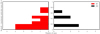 |
Fig. 6 Distribution of the sum of ionised and (maximum) molecular mass of the samples of single-degenerate and double-degenerate post-CE PNe analysed in this work. |
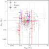 |
Fig. 7 Ionised vs. molecular mass of our post-CE PNe sample and the comparison, regular PNe sample. The further to the top and to the right a nebula is, the more massive it is. Dashed lines represent ‘isomasses’, indicating equal ionised + molecular mass; neglecting neutral atomic mass (see Sect. 4.3), individual nebulae run along these lines as their gas content is progressively ionised. |
Geometric means of the ionised + (maximum) molecular mass, linear momentum, and kinetic energy of the SD, DD, and regular samples analysed in this work, along with their respective geometric standard deviation (GSD) factors.
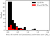 |
Fig. 8 Distribution of the sum of ionised and (maximum) molecular mass of the post-CE PNe sample, along with every PNe (both regular and post-CE PNe) analysed in this work. |
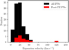 |
Fig. 9 Distribution of the expansion velocity of the post-CE PNe and regular PNe samples analysed in this work. |
5 Discussion
Simple considerations based on the mass lost by a star during the latter phase of the AGB, the briefness of the CE phase, and its sudden ejection would suggest that PNe hosting post-CE systems should be, on average, more massive than PNe arising from single stars (see Sect. 1 and Boffin & Jones 2019). However, previous work by Frew & Parker (2007) and Corradi et al. (2015) found the ionised mass of post-CE PNe to be lower, on average, than that of the general population of PNe. The analysis presented here considerably expands the sample size to one-fifth of the currently known post-CE PN population, and incorporatesthe molecular content of the nebulae, which is detected in only three systems (including NGC 6778, first reported in this work and analysed in Sect. 3). Considered globally, our results suggest a different conclusion: on average, PNe arising from single-degenerate (SD) systems seem to be just as massive as ‘regular’ PNe, whereas PNe arising from double-degenerate (DD) systems appear to be considerably more massive than both groups.
Differences between samples broaden when considering the linear momentum and kinetic energy of the outflows: as post-CE PNe also show higher expansion velocities (see Fig. 9), these magnitudes in post-CE PNe depart from the general population of PNe (see Table 5). This departure is especially notable in the case of DD systems, which are seemingly able to unbind a larger amount of matter than SD systems, and eject it at a higher velocity, thus imprinting their nebulae with an amount of linear momentum and kinetic energy that could help reveal their close-binary origin should the results of this work be confirmed and generalised by future research. In this respect,it is interesting to note the generally larger masses of the companions in DD systems – mostly over 0.6 M⊙ – than those in SD systems, which are mostly below 0.4 M⊙ (Hillwig, priv. comm.). Perhaps such a difference in companion mass (or the much larger difference in ultraviolet flux) could help to explain the observed discrepancy between the nebula ejected by post-CE SD and DD systems.
Our results further suggest a severe mismatch between observations and modelling. As summarised in Sect. 1, models of CE ejection tend to fail in unbinding the whole envelope without the aid of additional energy sources, such as recombination of the ionised region. The observational data instead seem to suggest that the unbound, expanding nebulae do not consist of the whole envelope of their AGB progenitor, but are instead considerably less massive. In this respect, reconstructing the stellar and orbital parameters at CE onset in these systems may help us to assess the fraction of the AGB envelope that is ejected, as well as the fraction of the orbital energy budget (the change in energy from orbital shrinkage) spent on unbinding and accelerating the nebula to the observed expansion velocity. While such an effort is undoubtedly plagued with caveats and large uncertainties, it can provide an ‘order of magnitude estimate’ to help guide theoretical modelling efforts.
Following the methodology described in Iaconi & De Marco (2019) and De Marco et al. (2011), we attempted to reconstruct the CE of the two SD systems, Abell 63 and Hen 2-155, and the two DD systems, Fg 1 and Hen 2-428, for which we have sufficient information on the orbital parameters. Table 6 shows the calculated efficiency α, the estimated AGB envelope mass of the primary star, Menv, the percentage of the envelope mass contained in the observed (ionised + molecular) nebula, fM, the orbital energy budget, ΔEorb, a rough estimate of the binding energy of the observed nebula with respect to the primary star core (assuming the λ parameter for AGBs provided by De Marco et al. 2011), its kinetic energy, and the percentage of the energy budget spent on unbinding and accelerating the nebula, fE, along with the references for the orbital parameters used.
If confirmed and generalised by additional data on the orbital parameters of other systems, these results seem to suggest that post-CE PNe arising from SD systems are substantially less massive than the envelope of their AGB progenitors, while those arising from DD systems are almost as massive (if not as massive, given such large uncertainties) as the envelope of their progenitor.
In any case, a problem akin to the long-standing issue of the missing mass of PNe (e.g. Kimura et al. 2012) persists. While one could inprinciple hypothesise that the mass we do not detect in ‘regular’ PNe is long gone, diluted in the ISM after millions of years of AGB wind, the fact that we cannot reconcile the observed mass of SD post-CE PNe with the mass of their envelopes at the time of CE interaction should constitute a warning about our incomplete understanding of the physics behind CE ejection. The missing mass in SD systems therefore leads to uncomfortable questions: If the primary star is of similar mass to normal post-AGB stars, and thus the mass of the nebula amounts to just a tiny fraction of the star’s envelope, then where is the rest of the envelope? Why are we unable to detect it somewhere in the vicinity of the star?
From a theoretical perspective, we can consider some possibilities. A fraction of the ejected mass could fall back and form a circumbinary disk (as in Kuruwita et al. 2016). If any of this material reaches the central stars, it could then be reprocessed, which could offer an explanation for the correlation between large abundance discrepancy factors and post-CE central stars in PNe Wesson et al. (2018). We can therefore wonder whether the CE itself could be not a unique, once-only process, albeit a long-lasting or episodic one. Models such as Grazing Envelope Evolution proposed by Soker (2015) and Shiber et al. (2017), in which the companion grazes the envelope of the RGB or AGB star while both the orbital separation and the giant radius shrink simultaneously over the course of tens to hundreds of years could perhaps help to explain the phenomenon. A model along these lines could, for instance, provide some insight into the case of NGC 2346, a particularly massive SD system with a relatively long post-CE orbital period in which the primary is believed to be a post-RGB star (Brown et al. 2019). At any rate, CE interaction would probably need to last long enough to allow for a considerable amount of the envelope mass of the primary to become diluted in the ISM beyond detectability in order for the presumed envelope mass at the time of a later ‘full’ CE ejection to be reconciled with the mass of the observed nebulae.
From an observational point of view, it could instead be interesting to study the infrared grain emission and the mass of dust in these objects. There exists the possibility that some amount of mass is contained in low-excitation neutral atoms, mainly in a PDR between the ionised region and an outer, molecule-rich domain. However, this is unlikely, given the general lack of molecular content observed in post-CE PNe reported in this work, which would suggest most of these nebulae are (almost) fully ionised. In fact, the only available data on a post-CE PN, a set of HERSCHEL/HIFI + PACS observations of NGC 2392, points to a very low neutral mass of the order of 2 × 10⁻³ M⊙ (Santander-García et al., in prep.). In spite of this, assessing the amount of low-excitation, neutral mass of a sample of post-CE PNe is still missing, and will be the subject of future work by our group.
CE and nebula ejection reconstruction parameters for a sample of post-CE PNe.
6 Conclusions
In this work, we gathered literature-available data on post-CE PNe including dereddened Hβ fluxes, and carried out observations of the molecular content of these objects, totalling a sample of 21 objects, roughly one-fifth of the total known population of post-CE PNe. We find a general lack of molecular content, with the exceptions of NGC 2346 and NGC 7293 in the literature, and our observations of NGC 6778. The data on the latter have allowed us to study the physical conditions of the molecular gas, as well as its spatial distribution, with the CO-rich gas located in a ring lying beyond the broken, clumpy ionised equatorial ring described by Guerrero & Miranda (2012), and expanding alongside it.
By means of the systematic calculation of the ionised and molecular masses of the whole sample of post-CE PNe, we conclude that post-CE PNe with SD central stars are as massive, on average, as their single star counterparts, whereas post-CE PNe with DD central stars are considerably more massive than both groups. The characteristic expansion velocities of post-CE PNe also seem higher than those of regular PNe. This in turn results in higher linear momenta and kinetic energy of the ejecta, which are particularly notable in the case of DD post-CE PNe.
We reconstructed the CE in the four systems (two SD and two DD) for which sufficient data on the orbital parameters are available, including the present masses of both stars, the orbital separation, and the presumed envelope mass of the primary at the time of CE. We find that DD systems eject more massive nebulae at higher velocities than SD systems do. However, we cannot reconcile the observed mass of the nebulae with the presumed mass of the progenitor star envelopes. Whereas PNe around DD systems would contain most (if not all) of the envelope of the progenitor AGB star, PNe in SD systems (as well as in ‘regular’ PNe) only show but a small fraction of the progenitor envelope. This in turn leads to an alarming question: if the remaining mass of the envelope of these systems is no longer on the surface of the now post-AGB star, and is not contained in the ejected CE (the nebula), where is it? The possibility that the large amount of missing mass in SD systems is in a hard-to-detect halo beyond the PN would in principle require CE interaction to last much longer than commonly found by models in order for the AGB star to be able to dispose of most of its envelope beyond detectability before shaping the visible nebula. Similarly, although the models of Vigna-Gómez et al. (2021) find that an appreciable quantity of the envelope may remain on the surface of the CE donor (the central star) following ejection, the discrepancies between observed and expected post-CE PN masses are too large to be explained by this scenario alone.
Future efforts to answer this question will in any case require new theoretical work on the one hand, and systematic observationsof the ionised and molecular content of the whole known population of post-CE PNe on the other, as well as observationally assessing the (unlikely) possibility that a significant fraction of these nebulae consists of low-excitation, neutral gas that is yet to be studied.
Acknowledgements
M.S.G., J.A., and V.B. acknowledge support by the Spanish Ministry of Science and Innovation (MICINN) through projects AxIN (grant AYA2016-78994-P) and EVENTs/Nebulae-Web (grant PID2019-105203GB-C21). D.J. acknowledges support from the Erasmus+ programme of the European Union under grant number 2020-1-CZ01-KA203-078200. D.J. also acknowledges support under grant P/308614 financed by funds transferred from the Spanish Ministry of Science, Innovation and Universities, charged to the General State Budgets and with funds transferred from the General Budgets of the Autonomous Community of the Canary Islands by the Ministry of Economy, Industry, Trade and Knowledge. This work has made use of data from the European Space Agency (ESA) mission Gaia (https://www.cosmos.esa.int/gaia), processed by the Gaia Data Processing and Analysis Consortium (DPAC, https://www.cosmos.esa.int/web/gaia/dpac/consortium). Funding for the DPAC has been provided by national institutions, in particular the institutions participating in the Gaia Multilateral Agreement.
Appendix A The mass of the regular comparison sample
Table A.1 shows the computed ionised and molecular masses of the sample of 97 regular PNe used for comparison in section 4.4 of the main paper.
Computed ionised and molecular masses of the regular comparison sample. Masses as determined here scale with distance squared.
Appendix B Parameters used in the analysis
Table B.1 shows the parameters used in this work for computing the ionised and molecular masses, linear momenta, and kinetic energy of the studied sample of post-CE PNe, as well as the regular PNe comparison sample.
Parameters used in the analsysis presented in this work.
References
- Aaquist, O. B. 1993, A&A, 267, 260 [NASA ADS] [Google Scholar]
- Abell, G. O. 1966, ApJ, 144, 259 [NASA ADS] [CrossRef] [Google Scholar]
- Aller, L. H., & Keyes, C. D. 1987, ApJS, 65, 405 [NASA ADS] [CrossRef] [Google Scholar]
- Bachiller, R., Forveille, T., Huggins, P. J., & Cox, P. 1997a, A&A, 324, 1123 [Google Scholar]
- Bachiller, R., Fuente, A., Bujarrabal, V., et al. 1997b, A&A, 319, 235 [NASA ADS] [Google Scholar]
- Balick, B., & Frank, A. 2002, ARA&A, 40, 439 [Google Scholar]
- Bandyopadhyay, R., Das, R., Mondal, S., & Ghosh, S. 2020, MNRAS, 496, 814 [NASA ADS] [CrossRef] [Google Scholar]
- Barker, T. 1978, ApJ, 219, 914 [CrossRef] [Google Scholar]
- Boffin, H. M. J., & Jones, D. 2019, The Importance of Binaries in the Formation and Evolution of Planetary Nebulae (Springer Nature) [Google Scholar]
- Boffin, H. M. J., Miszalski, B., Rauch, T., et al. 2012, Science, 338, 773 [Google Scholar]
- Bohigas, J. 2001, Rev. Mex. Astron. Astrofis., 37, 237 [NASA ADS] [Google Scholar]
- Bohigas, J. 2003, Rev. Mex. Astron. Astrofis., 39, 149 [NASA ADS] [Google Scholar]
- Bond, H. E. 1976, PASP, 88, 192 [NASA ADS] [CrossRef] [Google Scholar]
- Brown, A. J., Jones, D., Boffin, H. M. J., & Van Winckel, H. 2019, MNRAS, 482, 4951 [Google Scholar]
- Bujarrabal, V., Alcolea, J., & Planesas, P. 1992, A&A, 257, 701 [NASA ADS] [Google Scholar]
- Bujarrabal, V., Castro-Carrizo, A., Alcolea, J., & Sánchez Contreras, C. 2001, A&A, 377, 868 [NASA ADS] [CrossRef] [EDP Sciences] [Google Scholar]
- Cahn, J. H., Kaler, J. B., & Stanghellini, L. 1992, A&ASS, 94, 399 [Google Scholar]
- Castro-Carrizo, A., Bujarrabal, V., Fong, D., et al. 2001, A&A, 367, 674 [NASA ADS] [CrossRef] [EDP Sciences] [Google Scholar]
- Chamandy, L., Blackman, E. G., Frank, A., Carroll-Nellenback, J., & Tu, Y. 2020, MNRAS, 495, 4028 [NASA ADS] [CrossRef] [Google Scholar]
- Chornay, N., & Walton, N. A. 2020, A&A, 638, A103 [NASA ADS] [CrossRef] [EDP Sciences] [Google Scholar]
- Chornay, N., & Walton, N. A. 2021, A&A, 656, A110 [Google Scholar]
- Corradi, R. L., & Schwarz, H. E. 1993, A&A, 273, 247 [NASA ADS] [Google Scholar]
- Corradi, R. L. M., Sabin, L., Miszalski, B., et al. 2011, MNRAS, 410, 1349 [CrossRef] [Google Scholar]
- Corradi, R. L. M., Rodríguez-Gil, P., Jones, D., et al. 2014, MNRAS, 441, 2799 [NASA ADS] [CrossRef] [Google Scholar]
- Corradi, R. L. M., García-Rojas, J., Jones, D., & Rodríguez-Gil, P. 2015, ApJ, 803, 99 [NASA ADS] [CrossRef] [Google Scholar]
- Costa, R. D. D., Chiappini, C., Maciel, W. J., & de, J. A. 1996, A&AS, 116, 249 [NASA ADS] [CrossRef] [EDP Sciences] [Google Scholar]
- Danehkar, A., & Parker, Q. A. 2015, MNRAS, 449, L56 [NASA ADS] [CrossRef] [Google Scholar]
- Decin, L., Montargès, M., Richards, A. M. S., et al. 2020, Science, 369, 1497 [Google Scholar]
- de Marco, O., Hillwig, T. C., & Smith, A. J. 2008, AJ, 136, 323 [NASA ADS] [CrossRef] [Google Scholar]
- De Marco, O., Passy, J.-C., Moe, M., et al. 2011, MNRAS, 411, 2277 [CrossRef] [Google Scholar]
- Fong, D., Meixner, M., Castro-Carrizo, A., et al. 2001, A&A, 367, 652 [NASA ADS] [CrossRef] [EDP Sciences] [Google Scholar]
- Frew, D. J., & Parker, Q. A. 2007, in Asymmetrical Planetary Nebulae IV, 475 [Google Scholar]
- Frew, D. J., Parker, Q. A., & Bojičić, I. S. 2016, MNRAS, 455, 1459 [Google Scholar]
- Gaia Collaboration (Brown, A. G. A., et al.) 2021, A&A, 649, A1 [NASA ADS] [CrossRef] [EDP Sciences] [Google Scholar]
- García-Rojas, J., Peña, M., Morisset, C., Mesa-Delgado, A., & Ruiz, M. T. 2012, A&A, 538, A54 [NASA ADS] [CrossRef] [EDP Sciences] [Google Scholar]
- García-Segura, G., Ricker, P. M., & Taam, R. E. 2018, ApJ, 860, 19 [CrossRef] [Google Scholar]
- Gesicki, K., & Zijlstra, A. A. 2000, A&A, 358, 1058 [NASA ADS] [Google Scholar]
- Gesicki, K., Zijlstra, A. A., Acker, A., et al. 2006, A&A, 451, 925 [NASA ADS] [CrossRef] [EDP Sciences] [Google Scholar]
- Gesicki, K., Zijlstra, A. A., Hajduk, M., & Szyszka, C. 2014, A&A, 566, A48 [NASA ADS] [CrossRef] [EDP Sciences] [Google Scholar]
- Górny, S. K. 2014, A&A, 570, A26 [NASA ADS] [CrossRef] [EDP Sciences] [Google Scholar]
- Guerrero, M. A., & Miranda, L. F. 2012, A&A, 539, A47 [NASA ADS] [CrossRef] [EDP Sciences] [Google Scholar]
- Guerrero, M. A., Suzett Rechy-García, J., & Ortiz, R. 2020, ApJ, 890, 50 [NASA ADS] [CrossRef] [Google Scholar]
- Gurzadyan, G. A. 1997, The Physics and Dynamics of Planetary Nebulae (Springer-Verlag) [Google Scholar]
- Gussie, G. T.,& Taylor, A. R. 1989, PASP, 101, 873 [NASA ADS] [CrossRef] [Google Scholar]
- Gussie, G. T.,& Taylor, A. R. 1994, PASP, 106, 500 [NASA ADS] [CrossRef] [Google Scholar]
- Guzman-Ramirez, L., Gómez-Ruíz, A. I., Boffin, H. M. J., et al. 2018, A&A, 618, A91 [NASA ADS] [CrossRef] [EDP Sciences] [Google Scholar]
- Henry, R. B. C., Kwitter, K. B., Jaskot, A. E., et al. 2010, ApJ, 724, 748 [NASA ADS] [CrossRef] [Google Scholar]
- Hillwig, T. C., Jones, D., De Marco, O., et al. 2016, ApJ, 832, 125 [NASA ADS] [CrossRef] [Google Scholar]
- Höfner, S., & Olofsson, H. 2018, A&ARv, 26, 1 [Google Scholar]
- Hsia, C.-H., Zhang, Y., Kwok, S., & Chau, W. 2019, Ap&SS, 364, 32 [NASA ADS] [CrossRef] [Google Scholar]
- Huggins, P. J., & Healy, A. P. 1986, ApJ, 305, L29 [CrossRef] [Google Scholar]
- Huggins, P. J., & Healy, A. P. 1989, ApJ, 346, 201 [NASA ADS] [CrossRef] [Google Scholar]
- Huggins, P. J., Bachiller, R., Cox, P., & Forveille, T. 1996, A&A, 315, 284 [Google Scholar]
- Huggins, P. J., Bachiller, R., Planesas, P., Forveille, T., & Cox, P. 2005, ApJS, 160, 272 [NASA ADS] [CrossRef] [Google Scholar]
- Iaconi, R., & De Marco, O. 2019, MNRAS, 490, 2550 [Google Scholar]
- Ivanova, N. 2018, ApJ, 858, L24 [NASA ADS] [CrossRef] [Google Scholar]
- Ivanova, N., Justham, S., Chen, X., et al. 2013, A&ARv, 21, 59 [Google Scholar]
- Jones, D. 2020, Observational Constraints on the Common Envelope Phase (Springer), 123 [Google Scholar]
- Jones, D., & Boffin, H. M. J. 2017, Nat. Astron., 1, 0117 [Google Scholar]
- Jones, D., Lloyd, M., Santander-García, M., et al. 2010, MNRAS, 408, 2312 [Google Scholar]
- Jones, D., Boffin, H. M. J., Miszalski, B., et al. 2014, A&A, 562, 89 [Google Scholar]
- Jones, D., Boffin, H. M. J., Rodríguez-Gil, P., et al. 2015, A&A, 580, A19 [NASA ADS] [CrossRef] [EDP Sciences] [Google Scholar]
- Jones, D., Wesson, R., García-Rojas, J., Corradi, R. L. M., & Boffin, H. M. J. 2016, MNRAS, 455, 3263 [NASA ADS] [CrossRef] [Google Scholar]
- Kaler, J. B. 1970, ApJ, 160, 887 [NASA ADS] [CrossRef] [Google Scholar]
- Kaler, J. B., Kwitter, K. B., Shaw, R. A., & Browning, L. 1996, PASP, 108, 980 [NASA ADS] [CrossRef] [Google Scholar]
- Kimura, R. K., Gruenwald, R., & Aleman, I. 2012, A&A, 541, A112 [NASA ADS] [CrossRef] [EDP Sciences] [Google Scholar]
- Kingsburgh, R. L., & Barlow, M. J. 1994, MNRAS, 271, 257 [NASA ADS] [CrossRef] [Google Scholar]
- Kondrateva, L. N. 1979, Soviet Ast., 23, 193 [NASA ADS] [Google Scholar]
- Krabbe, A. C., & Copetti, M. V. F. 2005, A&A, 443, 981 [NASA ADS] [CrossRef] [EDP Sciences] [Google Scholar]
- Kuruwita, R. L., Staff, J., & De Marco, O. 2016, MNRAS, 461, 486 [NASA ADS] [CrossRef] [Google Scholar]
- Liu, X. W. 1998, MNRAS, 295, 699 [CrossRef] [Google Scholar]
- Liu, Y., Liu, X. W., Barlow, M. J., & Luo, S. G. 2004, MNRAS, 353, 1251 [NASA ADS] [CrossRef] [Google Scholar]
- Mavromatakis, F., Papamastorakis, J., & Paleologou, E. V. 2001, A&A, 374, 280 [NASA ADS] [CrossRef] [EDP Sciences] [Google Scholar]
- McCullough, P. R., Bender, C., Gaustad, J. E., Rosing, W., & Van Buren, D. 2001, AJ, 121, 1578 [NASA ADS] [CrossRef] [Google Scholar]
- McKenna, F. C., Keenan, F. P., Kaler, J. B., et al. 1996, PASP, 108, 610 [NASA ADS] [CrossRef] [Google Scholar]
- Meatheringham, S. J., Wood, P. R., & Faulkner, D. J. 1988, ApJ, 334, 862 [NASA ADS] [CrossRef] [Google Scholar]
- Milam, S. N., Woolf, N. J., & Ziurys, L. M. 2009, ApJ, 690, 837 [Google Scholar]
- Milanova, Y. V., & Kholtygin, A. F. 2009, Astron. Lett., 35, 518 [NASA ADS] [CrossRef] [Google Scholar]
- Miranda, L. F., Fernández, M., Alcalá, J. M., et al. 2000, MNRAS, 311, 748 [NASA ADS] [CrossRef] [Google Scholar]
- Miszalski, B., Acker, A., Moffat, A. F. J., Parker, Q. A., & Udalski, A. 2009, A&A, 496, 813 [NASA ADS] [CrossRef] [EDP Sciences] [Google Scholar]
- Miszalski, B., Corradi, R. L. M., Jones, D., et al. 2011a, in Asymmetric Planetary Nebulae 5 Conference [Google Scholar]
- Miszalski, B., Corradi, R. L. M., Boffin, H. M. J., et al. 2011b, MNRAS, 413, 1264 [NASA ADS] [CrossRef] [Google Scholar]
- Miszalski, B., Manick, R., Rauch, T., et al. 2019, PASA, 36, e042 [CrossRef] [Google Scholar]
- Munday, J., Jones, D., García-Rojas, J., et al. 2020, MNRAS, 498, 6005 [Google Scholar]
- Nandez, J. L. A., Ivanova, N., & Lombardi, J. C. J. 2015, MNRAS, 450, L39 [Google Scholar]
- O’dell, C. R. 1998, AJ, 116, 1346 [CrossRef] [Google Scholar]
- Ohlmann, S. T., Röpke, F. K., Pakmor, R., & Springel, V. 2016, ApJ, 816, L9 [Google Scholar]
- Öttl, S., Kimeswenger, S., & Zijlstra, A. A. 2014, A&A, 565, A87 [NASA ADS] [CrossRef] [EDP Sciences] [Google Scholar]
- Paczynski, B. 1976, in IAU Symp., 73, Structure and Evolution of Close Binary Systems, eds. P. Eggleton, S. Mitton, & J. Whelan, 75 [CrossRef] [Google Scholar]
- Pereyra, M., Richer, M. G., & López, J. A. 2013, ApJ, 771, 114 [NASA ADS] [CrossRef] [Google Scholar]
- Perinotto, M., Purgathofer, A., Pasquali, A., & Patriarchi, P. 1994, A&AS, 107, 481 [NASA ADS] [Google Scholar]
- Phillips, J. P. 1998, A&A, 340, 527 [NASA ADS] [Google Scholar]
- Phillips, J. P.,& Cuesta, L. 1999, AJ, 118, 2929 [CrossRef] [Google Scholar]
- Pottasch, S. R., & Bernard-Salas, J. 2015, A&A, 583, A71 [NASA ADS] [CrossRef] [EDP Sciences] [Google Scholar]
- Pottasch, S. R., Surendiranath, R., & Bernard-Salas, J. 2011, A&A, 531, A23 [NASA ADS] [CrossRef] [EDP Sciences] [Google Scholar]
- Reindl, N., Schaffenroth, V., Miller Bertolami, M. M., et al. 2020, A&A, 638, A93 [NASA ADS] [CrossRef] [EDP Sciences] [Google Scholar]
- Ricker, P. M.,& Taam, R. E. 2012, ApJ, 746, 74 [NASA ADS] [CrossRef] [Google Scholar]
- Rodríguez, M., Corradi, R. L. M., & Mampaso, A. 2001, A&A, 377, 1042 [NASA ADS] [CrossRef] [EDP Sciences] [Google Scholar]
- Sand, C., Ohlmann, S. T., Schneider, F. R. N., Pakmor, R., & Röpke, F. K. 2020, A&A, 644, A60 [NASA ADS] [CrossRef] [EDP Sciences] [Google Scholar]
- Santander-García, M., Bujarrabal, V., & Alcolea, J. 2012, A&A, 545, A114 [NASA ADS] [CrossRef] [EDP Sciences] [Google Scholar]
- Santander-García, M., Bujarrabal, V., Koning, N., & Steffen, W. 2015a, A&A, 573, A56 [NASA ADS] [CrossRef] [EDP Sciences] [Google Scholar]
- Santander-García, M., Rodríguez-Gil, P., Corradi, R. L. M., et al. 2015b, Nature, 519, 63 [Google Scholar]
- Santander-García, M., Bujarrabal, V., Alcolea, J., et al. 2017, A&A, 597, A27 [NASA ADS] [CrossRef] [EDP Sciences] [Google Scholar]
- Sarkar, G., & Sahai, R. 2021, ApJ, submitted, [arXiv:2108.02199] [Google Scholar]
- Scholz, F. W.,& Stephens, M. A. 1987, J. Am. Stat. Assoc., 82, 918 [Google Scholar]
- Schwarz, H. E., Monteiro, H., & Peterson, R. 2008, ApJ, 675, 380 [NASA ADS] [CrossRef] [Google Scholar]
- Shiber, S., Kashi, A., & Soker, N. 2017, MNRAS, 465, L54 [NASA ADS] [CrossRef] [Google Scholar]
- Soker, N. 2015, ApJ, 800, 114 [NASA ADS] [CrossRef] [Google Scholar]
- Stanghellini, L., & Kaler, J. B. 1989, ApJ, 343, 811 [NASA ADS] [CrossRef] [Google Scholar]
- Steffen, W., Koning, N., Wenger, S., Morisset, C., & Magnor, M. 2011, IEEE Trans. Visual. Comput. Graph., 17, 454 [CrossRef] [Google Scholar]
- Sterling, N. C., & Dinerstein, H. L. 2008, ApJS, 174, 158 [NASA ADS] [CrossRef] [Google Scholar]
- Storey, P. J., & Hummer, D. G. 1995, MNRAS, 272, 41 [NASA ADS] [CrossRef] [Google Scholar]
- Szyszka, C., Zijlstra, A. A., & Walsh, J. R. 2011, MNRAS, 416, 715 [NASA ADS] [Google Scholar]
- Torres-Peimbert, S., & Peimbert, M. 1977, Rev. Mex. Astron. Astrofis., 2, 181 [NASA ADS] [Google Scholar]
- Tsamis, Y. G., Barlow, M. J., Liu, X. W., Danziger, I. J., & Storey, P. J. 2003, MNRAS, 345, 186 [NASA ADS] [CrossRef] [Google Scholar]
- Tsamis, Y. G., Barlow, M. J., Liu, X. W., Storey, P. J., & Danziger, I. J. 2004, MNRAS, 353, 953 [NASA ADS] [CrossRef] [Google Scholar]
- Udalski, A., Szymanski, M. K., Soszynski, I., & Poleski, R. 2008, Acta Astron., 58, 69 [NASA ADS] [Google Scholar]
- Vigna-Gómez, A., Wassink, M., Klencki, J., et al. 2021, ArXiv e-prints, [arXiv:2107.14526] [Google Scholar]
- Villaver, E., Manchado, A., & García-Segura, G. 2002, ApJ, 581, 1204 [NASA ADS] [CrossRef] [Google Scholar]
- Wang, W., Liu, X. W., Zhang, Y., & Barlow, M. J. 2004, A&A, 427, 873 [NASA ADS] [CrossRef] [EDP Sciences] [Google Scholar]
- Webbink, R. F. 2008, Astrophys. Space Sci. Lib., 352, Common Envelope Evolution Redux, eds. E. F. Milone, D. A. Leahy, & D. W. Hobill (Springer), 233 [Google Scholar]
- Weinberger, R. 1989, A&AS, 78, 301 [NASA ADS] [Google Scholar]
- Wesson, R., Liu, X. W., & Barlow, M. J. 2005, MNRAS, 362, 424 [NASA ADS] [CrossRef] [Google Scholar]
- Wesson, R., Barlow, M. J., Corradi, R. L. M., et al. 2008, ApJ, 688, L21 [NASA ADS] [CrossRef] [Google Scholar]
- Wesson, R., Stock, D. J., & Scicluna, P. 2012, MNRAS, 422, 3516 [NASA ADS] [CrossRef] [Google Scholar]
- Wesson, R., Jones, D., García-Rojas, J., Boffin, H. M. J., & Corradi, R. L. M. 2018, MNRAS, 480, 4589 [Google Scholar]
- Zhang, Y., Liu, X. W., Luo, S. G., Péquignot, D., & Barlow, M. J. 2005, A&A, 442, 249 [NASA ADS] [CrossRef] [EDP Sciences] [Google Scholar]
See updated list with references to discovery papers in http://www.drdjones.net/bcspn/
By this same argument, PNe arising from CE ejection during the RGB should tend to be even more massive.
All Tables
Geometric means of the ionised + (maximum) molecular mass, linear momentum, and kinetic energy of the SD, DD, and regular samples analysed in this work, along with their respective geometric standard deviation (GSD) factors.
Computed ionised and molecular masses of the regular comparison sample. Masses as determined here scale with distance squared.
All Figures
|
Fig. 1 Detected (and tentatively detected) mm-wavelength emission at the position of the central star of NGC 6778. The systemic VLSR is 107.1 km s−1. An asterisk indicates that the velocity of the CN line complexes shown, with J = 3∕2–1/2 and J = 1∕2–1/2, are referenced to frequencies of 113.490985 GHz and 113.157347 GHz, respectively. The tentative CO+ line shown is a stack from the N = 2–1 group with J = 3∕2–3/2, 3/2–1/2, and 5/2–3/2. |
| In the text | |
|
Fig. 2 Detected 12CO and 13CO emission profiles at the position of the central star system of NGC 6778 (black), and corresponding SHAPE+SHAPEMOL model synthetic emission profiles (red). A Gaussian profile simulating H(38)α has been subtracted from the 12CO J = 1–0 emission in order to account for contamination from this recombination line (see text). |
| In the text | |
|
Fig. 3 Equatorial ring model (white) of the 12CO and 13CO emission of NGC 6778 overlaid on an image of the nebula taken with the NOT telescope (adapted from Guerrero & Miranda 2012). White crosses mark the observed offset positions, while associated insets show their corresponding 12CO J = 2–1 emission profiles (black) and SHAPE+SHAPEMOL model synthetic profiles (red). The HPBW of the IRAM 30m telescope at the 12CO J = 2–1 transition is indicated by the white circle. |
| In the text | |
|
Fig. 4 CN v = 0 J = 3∕2–1/2 and J = 1∕2–1/2 line complexes in NGC 6778. The red line indicates hyperfine structure modelling of CN emission (see Sect. 3.2). |
| In the text | |
|
Fig. 5 Ionised vs. molecular mass of our post-CE PNe sample. The further to the top and to the right a nebula is, the more massive it is. Dashed lines represent ‘isomasses’, indicating equal ionised + molecular mass; neglecting neutral atomic mass (see Sect. 4.3), individual nebulae run along these lines as their gas content is progressively ionised. |
| In the text | |
|
Fig. 6 Distribution of the sum of ionised and (maximum) molecular mass of the samples of single-degenerate and double-degenerate post-CE PNe analysed in this work. |
| In the text | |
|
Fig. 7 Ionised vs. molecular mass of our post-CE PNe sample and the comparison, regular PNe sample. The further to the top and to the right a nebula is, the more massive it is. Dashed lines represent ‘isomasses’, indicating equal ionised + molecular mass; neglecting neutral atomic mass (see Sect. 4.3), individual nebulae run along these lines as their gas content is progressively ionised. |
| In the text | |
|
Fig. 8 Distribution of the sum of ionised and (maximum) molecular mass of the post-CE PNe sample, along with every PNe (both regular and post-CE PNe) analysed in this work. |
| In the text | |
|
Fig. 9 Distribution of the expansion velocity of the post-CE PNe and regular PNe samples analysed in this work. |
| In the text | |
Current usage metrics show cumulative count of Article Views (full-text article views including HTML views, PDF and ePub downloads, according to the available data) and Abstracts Views on Vision4Press platform.
Data correspond to usage on the plateform after 2015. The current usage metrics is available 48-96 hours after online publication and is updated daily on week days.
Initial download of the metrics may take a while.