| Issue |
A&A
Volume 658, February 2022
|
|
|---|---|---|
| Article Number | A46 | |
| Number of page(s) | 7 | |
| Section | Numerical methods and codes | |
| DOI | https://doi.org/10.1051/0004-6361/202141732 | |
| Published online | 28 January 2022 | |
Intrinsic polarization of Wolf-Rayet stars due to the rotational modulation of the stellar wind
1
Department of Theoretical Physics and Astrophysics, Faculty of Science, Masaryk University, Kotlářská 2, Brno, Czech Republic
e-mail: This email address is being protected from spambots. You need JavaScript enabled to view it.
2
Institute of Theoretical Physics, Charles University, V Holešovičkách 2, Praha 8, Czech Republic
Received:
2
July
2021
Accepted:
2
November
2021
Abstract
Context. Fast rotating Wolf-Rayet stars are expected to be progenitors of long duration gamma-ray bursts. However, the observational test of this model is problematic. Spectral lines of Wolf-Rayet stars originate in expanding stellar wind, therefore a reliable spectroscopical determination of their rotational velocities is difficult. Intrinsic polarization of Wolf-Rayet stars due to the rotational modulation of the stellar wind may provide an indirect way to determine the rotational velocities of these stars. However, detailed wind models are required for this purpose.
Aims. We determine the intrinsic polarization of Wolf-Rayet stars from hydrodynamical wind models as a function of rotational velocity.
Methods. We used 2.5D hydrodynamical simulations to calculate the structure of rotating winds of Wolf-Rayet stars. The simulations account for the deformation of the stellar surface due to rotation, gravity darkening, and nonradial forces. From the derived models, we calculated the intrinsic stellar polarization. The mass loss rate was scaled to take realistic wind densities of Wolf-Rayet stars into account.
Results. The hydrodynamical wind models predict a prolate wind structure, which leads to a relatively low level of polarization. Even relatively large rotational velocities are allowed by observational constrains. The obtained wind structure is similar to that obtained previously for rotating optically thin winds.
Conclusions. Derived upper limits of rotational velocities of studied Wolf-Rayet stars are not in conflict with the model of long duration gamma-ray bursts.
Key words: stars: Wolf-Rayet / stars: rotation / polarization / stars: winds, outflows
© ESO 2022
1. Introduction
Classical Wolf-Rayet (WR) stars are massive stars that lost their hydrogen envelope during their evolution (Conti 1975; Chiosi et al. 1979; Sander et al. 2012). The collapse of fast rotating WR stars to a black hole could generate long duration gamma-ray bursts (Woosley 1993). In this context, Vink & de Koter (2005) proposed that fast rotating WR stars are progenitors of a long duration gamma-ray burst. However, a direct observational test of this model is difficult due to the problematic determination of rotational velocities of Wolf-Rayet stars. An estimation of rotational velocities from polarized light may provide an indirect way to test the nature of gamma-ray burst progenitors.
Winds of WR stars are ionized, consequently the light scattering on free electrons is an important source of opacity in the envelopes of these stars. As a result of light scattering on free electrons, an initially unpolarized beam coming from the stellar photosphere becomes linearly polarized. After scattering into the direction making an angle of Θ with respect to the incident beam, the ratio of intensities in the directions perpendicular and parallel to the plane of scattering (given by the directions of incident and scattered light) is 1 : cos2Θ (Chandrasekhar 1950). However, in spherically symmetric envelopes, the contribution of light polarized in different directions cancels out resulting in zero net polarization.
Most stars are known to be more or less spherical, but the rapid rotation could break the sphericity and lead to an axisymmetric density structure. If electron scattering takes place in an axisymmetric envelope, the intrinsic polarization occurs. From the measurement of Serkowski (1970), few WR stars have been found to be intrinsically polarized. McLean et al. (1979) discussed the dependence of the continuum polarization on wavelength in WR stars and discovered the decrease in polarization across the emission features.
To interpret the observed polarization, Brown & McLean (1977) developed an analytical method to compute the polarization due to optically thin electron scattering in axisymmetric envelopes. They assumed that the continuum polarization mainly depends on the inclination angle toward the line of sight, the geometry, and the optical depth. Cassinelli et al. (1987) rederived the polarization expression of Brown & McLean (1977) and added the depolarization correction factor of finite stellar size. Brown et al. (2000) showed that the depolarization factor has a negligible effect on the value for the polarization.
In the observational context (Schulte-Ladbeck 1994), there are several methods to separate the interstellar polarization and the intrinsic polarization, each being based on different assumptions. Stevance et al. (2018) applied Serkowski’s law to fit the interstellar polarization of WR93b and WR102. They conclude that these two stars are not intrinsically polarized, hence no line effect could be found, resulting from the dilution of continuum polarization by unpolarized lineflux. They placed the upper limit on the rotational velocity, which is lower than the value determined by Sander et al. (2012) from the shape of emission line profiles, where WR93b and WR102 are among a small group of WR stars with round emission line profiles, possibly implying fast rotation. High rotational velocities are required to form a collapsar, which is likely a source of long duration gamma-ray bursts (Woosley et al. 1999).
In this work, we discuss the limits of the rotational velocity of WR stars from polarimetry, in addition to the dependence of polarization on the inclination angle and rotational velocity. Our study is based on hydrodynamic stellar wind models of the selected WR stars WR93b and WR102 that include the effect of rotation. The obtained density was used to calculate the residual polarization. In Sect. 2, we describe the method by which the polarization was calculated. Sections 3–4 provide the discussion of the results with some comparison to the results of Stevance et al. (2018). In the last section, we provide the conclusions and some suggestions that might prove fruitful in the future.
2. Computational method
2.1. Hydrodynamic model
Stellar wind of hot stars is described by coupling radiative force with hydrodynamic model equations. The radiative force is based on the Sobolev approximation for stellar wind (Sobolev 1960; Castor 1974; Cranmer & Owocki 1995). The hydrodynamic model equations describing the wind expressed in spherical geometry are as follows in the axisymmetric case (Owocki et al. 1994):
 (1)
(1)
 (2)
(2)
 (3)
(3)
 (4)
(4)
 (5)
(5)
where ρ is the density of the fluid, vr, vθ, and vϕ are the velocity components in every direction, cs is the sound speed, and P is the gas pressure. For a star with a radius R⋆, mass M⋆, luminosity L⋆, and temperature T⋆, the external force gext is the vector sum of the line radiative force gline and the effective gravity geff.
The line force gline at the position r was obtained by integrating numerically the stellar intensity I over the solid angle Ω⋆ weighted by the velocity gradient (Cranmer & Owocki 1995)
![Mathematical equation: $$ \begin{aligned} \boldsymbol{g}_\text{ line}(\boldsymbol{r})=\frac{k \sigma _\text{ T}^{1-\alpha }}{ \rho (\boldsymbol{r})^{\alpha }c{ v}_{\text{ th}}^\alpha }\int _{\Omega _{\star }}(\boldsymbol{n}\cdot \mathbf \nabla [\boldsymbol{n}\cdot \boldsymbol{v}(\boldsymbol{r})])^{\alpha }\boldsymbol{n}\,I(\boldsymbol{n},\boldsymbol{r})\,\mathrm{d}\Omega . \end{aligned} $$](/articles/aa/full_html/2022/02/aa41732-21/aa41732-21-eq6.gif) (6)
(6)
Here, α and k are the Castor et al. (1975, hereafter CAK) and Abbott (1982) parameters for the radiative force, respectively, σT is the cross section due to Thomson scattering on free electrons, vth is the thermal velocity, and c is the speed of light. We note that the line force also depends on the dilution factor due to ionization which has been removed here as the δ parameter can be put equal to zero (see Table 1).
Adopted CAK parameters.
To solve the hydrodynamic model Eqs. (1)–(5), we used the VH-1 (Blondin et al. 1990) piecewise parabolic method (PPM) code coupled with the subroutine developed by Owocki et al. (1996) to determine the radiative force. The well-known PPM algorithm was developed by Colella & Woodward (1984), and it is the third-order finite difference scheme. The VH-1 code solves the hydrodynamic equations in 1D, 2D, and 3D planar, cylindrical, and spherical geometry. For our problem, we used 2.5D spherical geometry, with three velocity components (vr, vθ, vϕ), where the flow is specified along the radial and colatitudinal coordinate components (r and θ). The grid is discretized into ni = 320 zones in radius, from stellar surface rmin = R⋆ to rmax ≈ 10R⋆. The latitudinal direction is subdivided into nj = 100 equidistant zones from the north pole (θ = 0) to the south pole (θ = π).
The most important factor for hydrodynamic simulation of stellar winds is to define the lower boundary condition in the radial direction to introduce the oblate stellar surface due to rotation. Owocki et al. (1994) proposed a specified stair-casing boundary condition to solve this difficulty We have chosen the same configuration to formulate our problem. To assure a subsonic inflow of matter at the base of the wind, we set the base wind density to a constant value proportional to the mass loss rate Ṁ,
 (7)
(7)
whereas for the velocity component, we assume a subsonic outflow for polar velocity and rigid body rotation for the azimuthal velocity. To control the oblateness of the stellar surface, the radius was set as a function of colatitude θ and the ratio of rotational velocity and the critical velocity ω (Collins & Harrington 1966; Owocki et al. 1994)
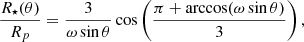 (8)
(8)
where R⋆(θ) is the surface radius and Rp is the polar radius. For the upper boundary, we set an outflow condition. Because of the symmetry, we set a reflecting boundary conditions (default from VH-1 code) in the latitudinal direction.
2.2. CAK parameter optimization
In order to make the numerical simulation of the two WR stars, we have to know the CAK parameters of the line force. To our knowledge, there has not been a previous calculation of line force parameters for these two stars. Therefore, to get the value of α and k, we required the terminal velocity and mass loss rate from observations. We varied the line force parameters to fit the observational values. We adopted the stellar parameters from Tramper et al. (2015) and Stevance et al. (2018, see Table 2). The selected values for CAK parameters are given in Table 1. The critical velocity is 1734 km s−1 for WR93b and 2286 km s−1 for WR102 (Stevance et al. 2018).
Adopted stellar and wind parameters.
The mass loss rate corresponding to the selected CAK parameters is 5.8 × 10⁻⁷ M⊙ yr−1 for WR93b and 4.7 × 10⁻⁷ M⊙ yr−1 for WR102, which is lower than what was derived from observations. Therefore, for the calculation of the polarization, we multiplied the density by the ratio of the observed mass loss given in Table 2 to the numerical mass loss from the hydrodynamic simulation. We multiplied the final density by a factor of 17 for WR93b and 24 for WR102. We could increase the mass loss rate to the observational values (e.g., including the δ parameter), but running the model with rotation leads to a nonphysical structure of the density and the velocity, as we could get higher velocity at the polar regions and some numerical instability occurred inside the computational domain. The obtained terminal velocity is about 6000 km s−1 for WR93b and around 8000 km s−1 for WR102.
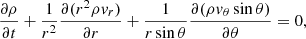
We ran the simulations for different rotational velocities. To check the influence of individual assumptions on the intrinsic polarization, we calculated several sets of wind models with an increasing level of complexity. First, we included radial force only leading to a compression effect as discussed by Bjorkman & Cassinelli (1993). Within these assumptions, an equatorial density enhancement forms, as found by Owocki et al. (1994). Second, we added the nonradial forces, which inhibit the formation of the disk (Owocki et al. 1996). In the most complex model, we also included the gravity darkening. Figure 1 shows the density contours as a function of the radius and colatitude for Vrot = 900 km s−1; the results are similar to those found by Owocki et al. (1996) and show a reduced density at the equator due to the gravity darkening and the effect of nonradial forces. Our aim is not to investigate the equatorial disk formation, but rather we want to make use of the hydrodynamic simulation in order to obtain the resulting polarization. In the following section, we show how the continuum polarization can be calculated from the wind density ρ derived from the hydrodynamic model.
 |
Fig. 1. Density (in g cm−3) contours of stellar wind of the star WR93b versus radius r and colatitude θ, in log scale spaced by 0.8 dex, denoted contour correspond to log(ρ)= − 11.2, for rotation Vrot = 1100 km s−1, with nonradial forces and gravity darkening. |
2.3. Polarization model
We intend to model the continuum polarization due to electron scattering, as we expect that the polarization will vanish in the emission lines. Polarization from radiation scattering depends on the integral of electron density and the volume of scattering. The analytic expression of the polarization was developed by Brown & McLean (1977), which depends on the inclination angle, optical depth, and geometry factor, as follows:
 (9)
(9)
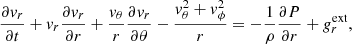
where  is the averaged Thomson scattering optical depth defined as the integral of the number density over the radius and the colatitudinal angle θ (as shown in Fig. 2, see also Brown et al. 1978),
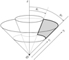 |
Fig. 2. Geometry of the plane of integration in spherical geometry (r,θ,ϕ) adopted from Brown et al. (2000). |
 (10)
(10)
The factor γ in Eq. (9) is given by
 (11)
(11)
where μ = cos θ, i is the inclination angle, and ne is the electron number density, which depends on the mass density ρ;
 (12)
(12)
where mH is the hydrogen atom mass and μe is the mean molecular weight per free electron (cf. also the calculation of polarization signatures in Kurfürst et al. 2020). To take the depolarization effect of finite stellar geometry into account, Cassinelli et al. (1987) introduced the correction factor 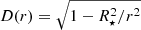 , and the polarization relation becomes the following:
 (13)
(13)
Stellar winds of WR stars are optically thick even in the vicinity of the sonic point. However, Eq. (13) accounts for just the polarization due to optically thin scattering. Therefore, we selected the lower limit of integration in Eq. (13) as r1 = 1.2R⋆ to exclude the optically thick part of the wind. The upper limit corresponds to the outer boundary of numerical simulations, r2 = 10R⋆.
2.4. Polarization due to surface temperature variation
The shape of the star changes due to the effect of rotation becomes oblate by the effect of centrifugal forces, and the emergent flux experiences a redistribution so that the polar regions become bright, and the equator becomes dark, what is known as the effect of gravity darkening. These effects can be specified by the known Roche and von Zeipel models for early type stars (Harrington & Collins 1968; Cranmer & Owocki 1995) and they affect the radiative intensity in the wind. The anisotropic intensity introduces an additional source of polarization.
The von Zeipel theorem (Collins 1963; Harrington & Collins 1968; Cranmer & Owocki 1995) shows that the local flux F(θ) on the surface of a rotating star is proportional to local effective gravity g(θ)
 (14)
(14)
where σB is the Boltzmann’s constant, Teff(θ) is the effective temperature depending on colatitude, and the magnitude of surface gravity is expressed as
![Mathematical equation: $$ \begin{aligned} g_\text{ eff}(\theta ) = \frac{GM_\star }{R_p^2}\left[\left(-\frac{1}{x^2}+\frac{8}{27}\omega ^2x\sin ^2\theta \right)^2+\left(\frac{8}{27}\omega ^2x\sin \theta \cos \theta \right)^2 \right]^\frac{1}{2} , \end{aligned} $$](/articles/aa/full_html/2022/02/aa41732-21/aa41732-21-eq17.gif) (15)
(15)
where  is the polar gravity term at the critical velocity. von Zeipel theorem does not provide the constant of proportionality and many authors (Collins 1963; Cranmer & Owocki 1995) fitted this constant as a function of ω; we assume this constant to be unity for simplicity.
If we assign the temperature to a point in the wind, the specific intensity I can be computed using
 (16)
(16)
where Bν is the Planck function of a black body.
From the work of Brown & McLean (1977, Eq. (20)), we have the intrinsic polarization
 (17)
(17)
where I1 ≪ I0 and P1 is the polarization of the scattered intensity I1
![Mathematical equation: $$ \begin{aligned} P_1=\frac{3\pi \sigma _T\sin ^2i}{16}\frac{\int _{r_1}^{r_2}\int _{\mu _1}^{\mu _2}n_\text{ e}(r)B_\nu (T_\text{ eff} (\theta ))[1-3\mu ^2]\mathrm{d}r\mathrm{d}\mu }{I_1}. \end{aligned} $$](/articles/aa/full_html/2022/02/aa41732-21/aa41732-21-eq21.gif) (18)
(18)
Replacing P1 and I0 and by their expressions, we get
 (19)
(19)
It is possible to add the depolarization D(r) effect due to finite stellar size as previously in Eq. (13).
2.5. Numerical integration
In order to numerically evaluate the integrals, we have used the trapezoidal rule as implemented in the Numpy library (Harris et al. 2020). Moreover, we used Pandas for data analysis (McKinney 2011) and Matplotlib for plotting (Hunter 2007).
Calculations were carried out for various values of rotational velocities. The results are shown in Figs. 3–6, where the polarization PR is plotted as a function of the inclination angle i for different fractions of the critical velocity.
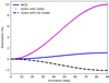 |
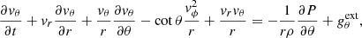
Fig. 3. Percentage polarization of WR93b from the model with radial force only (hydro with radial), nonradial forces, and gravity darkening (hydro with full model), compared to the model of the Ignace et al. (1996) wind compressed disk (WCD) for Vrot = 900 km s−1. |
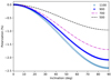 |
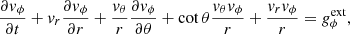
Fig. 5. Polarization of WR93b as a function of the inclination for different rotational velocities (denoted in the graph in units of km s−1) determined from the models including nonradial forces and gravity darkening. |
3. Results
Stevance et al. (2018) applied the simplified model of wind-compressed zones by Ignace et al. (1996) to investigate the dependence of the linear polarization on the stellar rotation. In our model, we included gravity darkening and oblateness of the star due to rotation effects; the model is based on the work of Cranmer & Owocki (1995) and Owocki et al. (1996).
Figures 3–6 show an increase in absolute values of the polarization by increasing the rotational velocity and the inclination angle. For higher rotational velocities, the departure from spherical symmetry becomes stronger, which leads to higher linear polarization. The inclination is another crucial parameter to observe the intrinsic polarization. When the inclination tends to zero, the system is viewed in the direction from the pole, the distribution of matter becomes symmetric with respect to the viewing direction, and the polarization drops to zero. The polarization reaches its maximum when the system is viewed equator on and when the angle coincides with the scattering plane. The signature of polarization is given by the geometry. The signature is positive for oblate disk-like geometry, while it becomes negative for prolate jet-like geometry.
The upper limit for rotation velocities was set to 19% and 10% (of the critical velocity) for both stars in the work of Stevance et al. (2018). This was determined from the observed value of the polarization, which is less than 0.077% for WR93 and less than 0.057% for WR102. For a comparison with their results, we additionally employed the analytical model by Ignace et al. (1996) to calculate the density structure of the wind. We calculated two sets of hydrodynamical models, one where the density was numerically computed including the radial force only, which corresponds to the analytical model. The second set of more realistic models includes the gravity darkening and nonradial components of the radiative force.
Due to a nonphysical structure which appears for low rotational velocities, we chose to calculate the polarization for the two stars with a higher rotational velocity than the ones employed by Stevance et al. (2018), as seen in Figs. 3–4. Figure 3 shows the intrinsic polarization for WR93b, where the values obtained from the hydrodynamic simulation with only radial forces of about 10% are higher than for the analytic model viewed equator on, while for the model with gravity darkening and nonradial forces, the polarization is 2% in absolute value. Figure 4 illustrates the variation of the polarization with inclination for WR102 star, the polarization from the hydrodynamic model is 18%, which is higher than from the analytical model (2.52%), while from nonradial forces and gravity darkening it is 0.61% in absolute value. In general, the polarization is positive for oblate density distribution and this shows that the plane of polarization is parallel to the symmetry axis. The polarization is negative when obtained from the model with gravity darkening, and this indicates that there is a higher density of material at the polar region than at the equatorial region, and the plane of polarization is perpendicular to the symmetry axis.
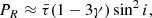
For the hydrodynamic model with the radial force only, we chose to integrate from the radius r1 = 1.2R⋆; the reason is that the oblateness of the stellar geometry, due to rotation and lower boundary conditions, rises the polarization degree and gives overestimated values. Wood et al. (1993) calculated the polarization for a Be star and they developed a relationship to get an estimate of the degree of the polarization. Applying Eq. (39),
 (20)
(20)
from their paper to the stellar parameters, we see that PR ≈ 8.6% for WR93b and PR ≈ 18% for WR102, which shows a good agreement with the hydrodynamic model.
Figures 5–6 show the variations of the polarization for the stars WR93 and WR102, respectively, and for different rotational velocities by adding nonradial forces and the gravity darkening. For the reason stated above, we chose to integrate from r1 = 1.2R⋆. The polarization is negative, which shows a prolate structure of the geometry, and for low rotational velocities, the intrinsic polarization tends to −0.95% for WR93b and to −0.17% for WR102. Increasing the rotational velocity decreases the net polarization; for a rotation about 60% of the critical velocity, we get PR = −2.4% and PR = −1.32% for WR93b and WR102, respectively.
To obtain the upper limits for rotational velocity, we carried out a logarithmic least square fitting for the model with nonradial forces and gravity darkening.
Table 3 shows a comparison of upper limits of rotational velocity, at the inclination angle 90° (edge-on), from our model and the model of Stevance et al. (2018).
Comparison between the fitted maximum observationally allowed rotational velocity (in km s−1) in this model and the model of Stevance et al. (2018).
Calculating the angular momentum j from the obtained rotational velocity, and comparing this with the threshold j ≥ 3 × 1016 cm2 s−1 of the collapsar derived by MacFadyen & Woosley (1999) in Table 3, the lower limits of angular momentum exceed the threshold of MacFadyen & Woosley (1999). Therefore, the studied WR stars may be progenitors of a long gamma-ray burst. This agrees with the results of Gräfener et al. (2012a), who determined the rotational velocities from photometry, and with the original results of Stevance et al. (2018).
In hydrodynamic simulations, we have considered an isothermal wind and assumed that variations of the effective temperature all over the stellar surface did not contribute to the polarization. In order to see the effect due to the change in the temperature, we computed the intrinsic polarization from Eq. (19), where the temperature changes due to the effective gravity (gravity darkening) and the number density is assumed to be radial dependent (ne(r) ∝ Ṁ/r2v(r)). For WR93b star with rotation ω = 20% of the critical velocity, the obtained polarization was found to be 0.0027%, which is smaller than the upper limit obtained from the observation (Stevance et al. 2018), and this means that this effect is not sufficient to break the symmetry of the star. On the other hand, for the critical rotation, the polarization can reach up to 14.52%. For WR102 with rotation ω = 20%, the polarization is similar to the previous star and has a value of 0.006%, and the rotation at critical velocity leads to a polarization with the value of 32.5%.
4. Discussion
We have determined the polarization due to electron scattering from hydrodynamical models of optically thin winds. The analysis involves several simplifications, including the neglect of the optically thick part of the wind on the density distribution and polarization which are perhaps the most significant ones. Therefore, in this section, we discuss the effect of the optical depth on the density distribution and polarization, as WR stars are known to have optical thick winds.
4.1. Density distribution
The adopted density distribution was derived from hydrodynamical models appropriate for winds which are optically thin in continuum. However, winds of WR stars may be optically thick and the radius of the hydrostatic core could be significantly lower than the radius of the unity mean optical depth (Gräfener et al. 2012b; Poniatowski et al. 2021). If we consider the effect of gravity darkening, the density has a prolate distribution; however, in the optically thick regime, the radiative diffusion effects may further complicate the structure of the flow (Gayley 2004). Using the model outlined in Owocki et al. (1998), and Dwarkadas & Owocki (2002), which was adopted to optically thick winds, the mass flux is expressed as
 (21)
(21)
where ṁ(0) is the mass flux at the pole. The mass conservation implies that in addition to the mass flux, the wind speed would be modified by the rotational effect. The wind terminal speed is expressed as a function of colatitude,
 (22)
(22)
where v∞(0) is the terminal speed at the pole. For ω = 20%, the polarization is −0.48% and −1.03% for WR93b and for WR102, respectively; also, at the critical rotation, the polarization is −20.5% for WR93b and −43% for WR102. Comparing this with the hydrodynamic model including nonradial forces and gravity darkening, the polarization values showed comparable results, where, for example, ω = 30%, PR = −1.1%, and PR = −2.3% and from hydrodynamic with nonradial forces and gravity darkening PR = −0.95% and PR = −0.11% for WR93b and for WR102, respectively. We note that in the hydrodynamic model, we integrated from r = 1.2R⋆ as mentioned earlier. This indicates that the effect of modifying the wind density due to the optical thickness of WR star winds does not significantly change the main results of our paper.
4.2. Optical depth
The polarization does not only depend on the inclination or rotational velocity, but it also depends on the opacity of the medium. In our model, we assumed the optical thin regime, but using Monte Carlo radiative transfer, Carlos-Leblanc et al. (2019) show that the polarization increases by increasing the optical depth (τ > 1). Due to their high mass loss rate, WR stars have an optical thick wind even to the electron scattering. To investigate the effect of the optical depth, using a more detailed treatment of the polarized radiative transfer, for instance with the Monte Carlo method of the radiative transfer, is needed. A work is under way using the latter method in couple with the hydrodynamic model, but we note that our models account for the strongest effect which is due to the last scattering in an optically thin envelope.
We assumed that the stars produce unpolarized light, which propagates into the wind where each photon scatters once at most. This is a simplification, especially for the winds of WR stars with a high density. However, multiple scattering leads to depolarization; therefore, we selected integration radii outside the optically thick envelope.
4.3. Magnetic field effect and the ionization structure
In this work, we did not consider the magnetic field. As a result of the magnetic field, the wind flows along the field lines, the mass-flux depends on the magnetic field tilt, and the circumstellar environment deviates from spherical symmetry (Ud-Doula et al. 2008; Küker 2017). This should also result in intrinsic polarization. Also, we neglected the variations in electron density due to the change of ionization, which is a reasonable approximation when the surface abundances are dominated by helium and for relatively high effective temperatures.
To maintain the acceleration around the sonic point, high effective temperatures are needed (Gräfener & Hamann 2005), which allow for strong dependence of the iron peak element opacity on the temperature in WR stars. As showed by Gräfener & Hamann (2005), the “Iron Bump” opacity may lead to an optically thick wind. Another factor that could impact the wind optical depth is the combination between the Eddington limit and the limit of rotation. As discussed by Maeder & Meynet (2000), and Gräfener (2021) and known as the ΓΩ limit, for high Γ, just moderate rotation is sufficient to increase the mass loss rates and as consequence the wind becomes optically thick. These effects can further modify our results.
5. Conclusions
In this work, we used the outputs of the density distribution from the hydrodynamic model to calculate the intrinsic polarization for WR93 and WR102 for different rotational velocities. Oblate density distribution leads to a positive polarization, while prolate distribution leads to a negative polarization, and this agrees with the model predicted by Brown & McLean (1977). The intrinsic polarization strongly depends on the rotational velocities and the inclination.
Based on our assumption, where we have scaled the density to take realistic values of mass-loss rates of studied stars into account, we show that fast rotation leads to a prolate density distribution around WR stars. This produces just a weak polarization signature, which is smaller than the upper limit of polarization from observations for low rotational velocities. Therefore, the limits of rotational velocities of WR stars from polarization do not contradict models of a long duration gamma-ray burst, according to which the fast rotating WR stars are progenitors of gamma ray bursts.
Acknowledgments
The authors thank Profs. R. Ignace and S. Owocki for discussion. The access to computing and storage facilities owned by parties and projects contributing to the National Grid Infrastructure MetaCentrum, provided under the program ‘Projects of Large Infrastructure for Research, Development, and Innovations’ (LM2010005) is appreciated. This research was supported by the grant Primus/SCI/17.
References
- Abbott, D. C. 1982, ApJ, 259, 282 [Google Scholar]
- Bjorkman, J. E., & Cassinelli, J. P. 1993, ApJ, 409, 429 [NASA ADS] [CrossRef] [Google Scholar]
- Blondin, J. M., Kallman, T. R., Fryxell, B. A., & Taam, R. E. 1990, ApJ, 356, 591 [Google Scholar]
- Brown, J. C., & McLean, I. S. 1977, A&A, 57, 141 [NASA ADS] [Google Scholar]
- Brown, J. C., McLean, I. S., & Emslie, A. G. 1978, A&A, 68, 415 [NASA ADS] [Google Scholar]
- Brown, J. C., Ignace, R., & Cassinelli, J. P. 2000, A&A, 356, 619{\newpage} [NASA ADS] [Google Scholar]
- Carlos-Leblanc, D., St-Louis, N., Bjorkman, J. E., & Ignace, R. 2019, MNRAS, 489, 2873 [NASA ADS] [CrossRef] [Google Scholar]
- Cassinelli, J. P., Nordsieck, K. H., & Murison, M. A. 1987, ApJ, 317, 290 [NASA ADS] [CrossRef] [Google Scholar]
- Castor, J. L. 1974, MNRAS, 169, 279 [NASA ADS] [CrossRef] [Google Scholar]
- Castor, J. I., Abbott, D. C., & Klein, R. I. 1975, ApJ, 195, 157 [Google Scholar]
- Chandrasekhar, S. 1950, Radiative Transfer (Oxford: Clarendon Press) [Google Scholar]
- Chiosi, C., Nasi, E., & Bertelli, G. 1979, A&A, 74, 62 [NASA ADS] [Google Scholar]
- Colella, P., & Woodward, P. R. 1984, J. Comput. Phys., 54, 174 [NASA ADS] [CrossRef] [Google Scholar]
- Collins, G. W. I. 1963, ApJ, 138, 1134 [NASA ADS] [CrossRef] [Google Scholar]
- Collins, G. W. I., & Harrington, J. P. 1966, ApJ, 146, 152 [NASA ADS] [CrossRef] [Google Scholar]
- Conti, P. S. 1975, Memoires Soc. R. Sci. Liege, 9, 193 [NASA ADS] [Google Scholar]
- Cranmer, S. R., & Owocki, S. P. 1995, ApJ, 440, 308 [NASA ADS] [CrossRef] [Google Scholar]
- Dwarkadas, V. V., & Owocki, S. P. 2002, ApJ, 581, 1337 [NASA ADS] [CrossRef] [Google Scholar]
- Gayley, K. G. 2004, Stellar Rotation, A. Maeder, & P. Eenens, 215, 527 [Google Scholar]
- Gräfener, G. 2021, A&A, 647, A13 [NASA ADS] [CrossRef] [EDP Sciences] [Google Scholar]
- Gräfener, G., & Hamann, W.-R. 2005, A&A, 432, 633 [NASA ADS] [CrossRef] [EDP Sciences] [Google Scholar]
- Gräfener, G., Vink, J. S., Harries, T. J., & Langer, N. 2012a, A&A, 547, A83 [NASA ADS] [CrossRef] [EDP Sciences] [Google Scholar]
- Gräfener, G., Owocki, S. P., & Vink, J. S. 2012b, A&A, 538, A40 [NASA ADS] [CrossRef] [EDP Sciences] [Google Scholar]
- Harrington, J. P., & Collins, G. W. I. 1968, ApJ, 151, 1051 [NASA ADS] [CrossRef] [Google Scholar]
- Harris, C. R., Millman, K. J., van der Walt, S. J., et al. 2020, Nature, 585, 357 [NASA ADS] [CrossRef] [Google Scholar]
- Hunter, J. D. 2007, Comput. Sci. Eng., 9, 90 [NASA ADS] [CrossRef] [Google Scholar]
- Ignace, R., Cassinelli, J. P., & Bjorkman, J. E. 1996, ApJ, 459, 671 [NASA ADS] [CrossRef] [Google Scholar]
- Küker, M. 2017, Astron. Nachr., 338, 868 [CrossRef] [Google Scholar]
- Kurfürst, P., Pejcha, O., & Krtička, J. 2020, A&A, 642, A214 [NASA ADS] [CrossRef] [EDP Sciences] [Google Scholar]
- MacFadyen, A. I., & Woosley, S. E. 1999, ApJ, 524, 262 [NASA ADS] [CrossRef] [Google Scholar]
- Maeder, A., & Meynet, G. 2000, A&A, 361, 159 [NASA ADS] [Google Scholar]
- McKinney, W. 2011, Python for High Performance and Scientific Computing, 14 [Google Scholar]
- McLean, I. S., Coyne, G. V., Frecker, S. J. J. E., & Serkowski, K. 1979, ApJ, 231, L141 [NASA ADS] [CrossRef] [Google Scholar]
- Owocki, S. P., Cranmer, S. R., & Blondin, J. M. 1994, ApJ, 424, 887 [NASA ADS] [CrossRef] [Google Scholar]
- Owocki, S. P., Cranmer, S. R., & Gayley, K. G. 1996, ApJ, 472, L115 [Google Scholar]
- Owocki, S. P., Cranmer, S. R., & Gayley, K. G. 1998, Ap&SS, 260, 149 [Google Scholar]
- Poniatowski, L. G., Sundqvist, J. O., Kee, N. D., et al. 2021, A&A, 647, A151 [NASA ADS] [CrossRef] [EDP Sciences] [Google Scholar]
- Sander, A., Hamann, W. R., & Todt, H. 2012, A&A, 540, A144 [NASA ADS] [CrossRef] [EDP Sciences] [Google Scholar]
- Schulte-Ladbeck, R. E. 1994, Ap&SS, 221, 347 [NASA ADS] [CrossRef] [Google Scholar]
- Serkowski, K. 1970, ApJ, 160, 1083 [NASA ADS] [CrossRef] [Google Scholar]
- Sobolev, V. V. 1960, Moving Envelopes of Stars (Cambridge: Harvard University Press) [Google Scholar]
- Stevance, H. F., Ignace, R., Crowther, P. A., et al. 2018, MNRAS, 479, 4535 [NASA ADS] [CrossRef] [Google Scholar]
- Tramper, F., Straal, S. M., Sanyal, D., et al. 2015, A&A, 581, A110 [NASA ADS] [CrossRef] [EDP Sciences] [Google Scholar]
- Ud-Doula, A., Owocki, S. P., & Townsend, R. H. D. 2008, MNRAS, 385, 97 [NASA ADS] [CrossRef] [Google Scholar]
- Vink, J. S., & de Koter, A. 2005, A&A, 442, 587 [NASA ADS] [CrossRef] [EDP Sciences] [Google Scholar]
- Wood, K., Brown, J. C., & Fox, G. K. 1993, A&A, 271, 492 [NASA ADS] [Google Scholar]
- Woosley, S. E. 1993, ApJ, 405, 273 [Google Scholar]
- Woosley, S. E., Eastman, R. G., & Schmidt, B. P. 1999, ApJ, 516, 788 [NASA ADS] [CrossRef] [Google Scholar]
All Tables
Comparison between the fitted maximum observationally allowed rotational velocity (in km s−1) in this model and the model of Stevance et al. (2018).
All Figures
|
Fig. 1. Density (in g cm−3) contours of stellar wind of the star WR93b versus radius r and colatitude θ, in log scale spaced by 0.8 dex, denoted contour correspond to log(ρ)= − 11.2, for rotation Vrot = 1100 km s−1, with nonradial forces and gravity darkening. |
| In the text | |
|
Fig. 2. Geometry of the plane of integration in spherical geometry (r,θ,ϕ) adopted from Brown et al. (2000). |
| In the text | |
|
Fig. 3. Percentage polarization of WR93b from the model with radial force only (hydro with radial), nonradial forces, and gravity darkening (hydro with full model), compared to the model of the Ignace et al. (1996) wind compressed disk (WCD) for Vrot = 900 km s−1. |
| In the text | |
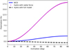 |
Fig. 4. As in Fig. 3, but for WR102. |
| In the text | |
|
Fig. 5. Polarization of WR93b as a function of the inclination for different rotational velocities (denoted in the graph in units of km s−1) determined from the models including nonradial forces and gravity darkening. |
| In the text | |
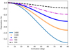 |
Fig. 6. As in Fig. 5, but for WR102. |
| In the text | |
Current usage metrics show cumulative count of Article Views (full-text article views including HTML views, PDF and ePub downloads, according to the available data) and Abstracts Views on Vision4Press platform.
Data correspond to usage on the plateform after 2015. The current usage metrics is available 48-96 hours after online publication and is updated daily on week days.
Initial download of the metrics may take a while.