| Issue |
A&A
Volume 698, May 2025
|
|
|---|---|---|
| Article Number | A225 | |
| Number of page(s) | 6 | |
| Section | Numerical methods and codes | |
| DOI | https://doi.org/10.1051/0004-6361/202553921 | |
| Published online | 17 June 2025 | |
Polarization of light from fast-rotating Wolf–Rayet stars: Monte Carlo simulations compared to the analytical formula
1
Department of Theoretical Physics and Astrophysics, Faculty of Science, Masaryk University,
Kotlářská 2,
Brno,
Czech Republic
2
Astronomical Institute of the Czech Academy of Sciences,
Fričova 298,
251 65
Ondřejov,
Czech Republic
★ Corresponding author: slah@physics.muni.cz
Received:
27
January
2025
Accepted:
27
April
2025
Context. Fast-rotating Wolf–Rayet (WR) stars are potential progenitors of long gamma-ray bursts, but observational verification is challenging. Spectral lines from their expanding stellar wind obscure accurate rotational velocity measurements. Intrinsic polarization from wind rotation may help to determine rotational speeds. However, this procedure requires precise wind models.
Aims. Our study aims to investigate the intrinsic polarization due to the rotational distortion of WR winds considering multiplescattering of photons and compare it to a single-scattering model, in which we use an analytical expression of the polarization.
Methods. We studied the polarization signatures resulting from the prolate structure of rotating winds of two WR stars using a 3D Monte Carlo radiative transfer code Hyperion. We estimated the intrinsic polarization resulting from multiple-scattering in WR winds for different rotational velocities, inclination angles, and mass-loss rates.
Results. Our results indicate that at a rotation rate of less than 50% of the critical rate, the intrinsic polarization from multiplescattering is close to that of a single-scattering model. However, at higher rotation velocities, the polarization from multiple-scattering increases with inclination up to 40°, while it decreases for inclinations higher than about 60°. This dependence is inconsistent with the single-scattering model. We also discuss the effect of the mass-loss rate on the polarization and find that the polarization changes linearly with the mass-loss rate. However, it is important to note that the relationship between polarization and mass-loss rate may vary for different types of stars.
Conclusions. The results have implications for future studies of stellar winds and mass loss and may help to improve our understanding of the complex environments of massive stars. Our research offers valuable information on the complex polarization patterns observed in stellar winds, emphasizing the significance of accounting for the influence of multiple-scattering when interpreting observations.
Key words: gamma-ray burst: general / stars: massive / stars: mass-loss / stars: rotation / stars: winds, outflows / stars: Wolf–Rayet
© The Authors 2025
 Open Access article, published by EDP Sciences, under the terms of the Creative Commons Attribution License (https://creativecommons.org/licenses/by/4.0), which permits unrestricted use, distribution, and reproduction in any medium, provided the original work is properly cited.
This article is published in open access under the Subscribe to Open model. Subscribe to A&A to support open access publication.
1 Introduction
Classical Wolf–Rayet (WR) stars correspond to massive stars in a late evolutionary stage that are characterized by having lost their hydrogen envelope during their evolution (Conti 1975; Chiosi et al. 1979; Sander et al. 2012). There are several possibilities for how these stars could lose their envelopes. The classical scenarios include mass-loss by line-driven winds (Groh et al. 2013) and binary interactions (Vanbeveren et al. 2007). This would imply that at low metallicities, where line-driven winds become weaker, the binary channel dominates, and only the most massive stars reach the domain of WR stars (Gormaz-Matamala et al. 2024). However, the absence of binary companions in Small Magellanic Cloud WR stars (Schootemeijer et al. 2024) indicates the need for an additional mass-loss mechanism that operates in single stars. On the other hand, the WR phenomenon is defined purely on spectroscopic grounds, and this definition can play a role in the apparent independence of the binary WR star fraction on metallicity (Shenar et al. 2020).
WR stars have gained significant attention in astrophysics due to their potential role in various cosmic phenomena. Notably, the collapse of rapidly rotating WR stars into black holes has been proposed as a mechanism for generating long-duration gamma-ray bursts (LGRBs, Woosley 1993). Building on this concept, Vink & de Koter (2005) and Gräfener et al. (2012, among others) suggested that fast-rotating WR stars could be the progenitors of LGRBs. This is supported by radiative transfer models of supernovae explosions associated with gamma-ray bursts, which indicate the breaking of spherical symmetry possibly connected with rotation of the progenitor (Dessart et al. 2017). However, directly testing this hypothesis presents challenges, primarily due to the difficulty in accurately measuring the rotational velocities of WR stars. These stars typically show emission lines originating in their expanding envelopes (Crowther et al. 1995; Hamann et al. 2006), which prevents a straightforward detection of rotational broadening.
An alternative approach to investigate the rotation of WR stars, and thus the origin of gamma-ray bursts, involves analyzing polarized light from these stars, which may indirectly reveal information about their rotation. As a result of stellar rotation, winds cease to be spherically symmetric, with stronger outflows coming from the polar regions due to the effect of nonradial forces and gravity darkening (Owocki et al. 1996; Petrenz & Puls 2000). The asymmetry can be detected from polarization. The winds surrounding WR stars are highly ionized, making electron scattering a significant source of opacity in their stellar envelopes. This scattering process transforms the initially unpolarized light from the star’s photosphere into linearly polarized light. When light scatters at an angle,  , relative to its original direction, the ratio of intensities perpendicular and parallel to the scattering plane (defined by the incident and scattered light directions) is
  (Chandrasekhar 1950). In a perfectly spherically symmetric envelope, the polarization contributions from different directions would cancel each other out, resulting in zero net polarization. However, any asymmetry in the stellar wind or envelope can lead to detectable polarization, potentially providing insights into the star’s structure and rotation.
Theoretical modeling of the polarization due to single-scattering of a point source radiation illuminating a circumstellar envelope has been studied by Brown & McLean (1977). Their formula was extended to include the depolarization effect (Cassinelli et al. 1987; Brown et al. 1989) and stellar occultation (Brown & Fox 1989). These models compute the polarization based on the simplified assumption that the photons are scattered only once. However, it has been shown by Wood et al. (1996a,b), Hoffman et al. (2003), and Townsend (2012) that the polarization obtained from Monte Carlo radiative transfer, which accounts for multiple-scattering, differs from that obtained using the single-scattering model.
In our previous work (Abdellaoui et al. 2022), we applied Brown-McLean’s formula to compute the polarization from a single-scattering model, assuming optically thin stellar winds from the hydrodynamic calculations. However, in reality, the wind of WR stars is optically thick (Gräfener et al. 2017; Grassitelli et al. 2018). To achieve a more realistic model of the polarization of WR stars, it is necessary to consider the effects of multiple photon scattering. Monte Carlo radiative transfer (MCRT) codes are widely used to model such complex environments because they can account for asymmetric, nonuniform, and optically thick scattering in media.
In this work, we present a study based on the Monte Carlo (MC) method to investigate the polarization signatures resulting from the stellar wind of two WR stars. We compare the results with the analytical formulation for a single-scattering model (Brown & McLean 1977).
2 Numerical methods
2.1 Wind model setup
WR stars possess dense and thick winds (Nugis & Lamers 2002; Gräfener et al. 2017; Grassitelli et al. 2018), making it challenging to use hydrodynamic models, such as the ones utilized by Abdellaoui et al. (2022), to accurately predict polarization. These models encounter difficulties in considering the impact of the optically thick wind.
To address these complexities, we used an alternative model developed by Dwarkadas & Owocki (2002). This model is specifically tailored to tackle the extreme conditions characteristic of WR stars, accounting for both gravity darkening and the influence of optically thick winds. Consequently, this model is better suited for our polarization calculations. The mass flux is considered to be higher at polar regions decreasing toward the equator, due to the gravity-darkening effect. Using the model of Dwarkadas & Owocki (2002), the stellar wind velocity is expressed as
 (1)
and the mass flux,
(1)
and the mass flux,  , as
, as
 (2)
(2)
The wind density distribution (see Fig. 1) is given by
 (3)
(3)
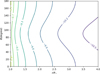 |
Fig. 1 Wind density contours for the rotation rates |


 is the wind massloss rate,
  is the rotation rate (the ratio of angular velocity,
  , to the critical velocity), r is the radial distance in the spherical coordinate,
  is colatitude, and
  is the so-called
  -velocity law (see e.g. Lamers & Cassinelli 1999) described as
  , where
  is the initial wind velocity,
  is the terminal wind velocity, the exponent
  is a parameter describing the steepness of the velocity law fixed to the standard value
  , and
, and  is the stellar radius. For the region located between the point source and the base of the wind at
  , we assumed zero density. The critical angular velocity was calculated using
 (4),
with G being the gravitational constant. Table 1 shows the stellar and wind parameters of two WR stars used in this work.
(4),
with G being the gravitational constant. Table 1 shows the stellar and wind parameters of two WR stars used in this work.
Adopted stellar and wind parameters (Tramper et al. 2015; Stevance et al. 2018)
2.2 Continuum polarization calculation
2.2.1 Analytical calculations
To compute the polarization analytically in the winds of WR stars, we used the mathematical expression derived by Brown & McLean (1977) as
 (5)
where
(5)
where  is the Thomson scattering cross section,
  is the cosine of the polar angle,
  is the electron number density of the envelope, and i is the inclination angle of the symmetry axis with respect to the observer (cf. also the calculation of polarization signatures in Kurfürst et al. 2020).
  is the depolarization factor introduced by Cassinelli et al. (1987) as
  . The lower limit of integration is
  and the upper limit corresponds to the outer boundary of numerical simulations,
  .
.
Since the wind of WR stars is optically thick to electron scattering, we included the attenuation factor  (McLean 1979; Friend & Cassinelli 1986), where the optical depth,
  is given as
 (6)
(6)
The analytical expression of polarization becomes
 (7)
(7)
2.2.2 Monte Carlo calculations
The continuum polarization in hot star winds appears due to the scattering of photons by free electrons in an axisymmetric environment. The degree of polarization depends on several parameters, such as the optical depth and the inclination. The polarization state of radiation can be described by the Stokes vector, S, as follows,
 (8),
where I is the radiation intensity, Q and U represent the linear polarization, and V describes the circular polarization. The degree of linear polarization can be written as
(8),
where I is the radiation intensity, Q and U represent the linear polarization, and V describes the circular polarization. The degree of linear polarization can be written as
 (9)
and the angle of linear polarization is given by
(9)
and the angle of linear polarization is given by
 (10)
(10)
To record the change in polarization state during a scattering event, the Stokes vector is multiplied by the Müller matrix, M, corresponding to the event. It is assumed that the reference direction lies in the scattering plane and the plane orthogonal to the propagation direction. The components of the Müller matrix depend on the geometry of the scattering event, the physical properties of the scatterer, and often on the wavelength. The Müller matrix for rotation is written as (Collins 1989)
 (11).
(11).
For electron scattering, the Müller matrix can be expressed as a function of the scattering angle,  (Chandrasekhar 1950; Code & Whitney 1995; Peest et al. 2017):
 (12).
(12).
We used a 3D MCRT code Hyperion1 (Robitaille 2011) to calculate the polarization of two fast-rotating WR stars (WR 93b and WR 102, see Table 1), considering multiple-scattering. The code was developed to cover a wide range of problems. It is parallelized and solves the radiative transfer equation in various geometries, including Cartesian, cylindrical, polar, spherical, and adaptive Cartesian grids. The code also computes the temperature, spectral energy distribution, and images. The MC method solves the radiative transfer equation by simulating photon packages and using a ray tracing approach.
Hyperion code uses a four-element Müller matrix to calculate the polarization, taking into account multiple-scattering. After the photon has left the computational domain, the reference direction of the Stokes vector is adjusted to align with the star’s rotational axis. This alignment allows us to group the photons into specific observer bins corresponding to the appropriate inclination. A total of 107 photons were utilized for imaging and ray tracing. For a direct comparison between our MC simulations and the analytical formula by Brown & McLean (1977), the stars are represented as point sources of known radius (  ), luminosity (
  ), and effective temperature (
  ), located at the center of the computational domain (i.e., the winds of the WR stars) with the lower boundary at
  and the outer boundary at
  . This assumption separates the effects of scattering in the stellar wind, which is the primary focus of our work, and ensures that any differences between the simulations and the analytical outcomes can be linked to the scattering physics rather than the geometry of the source. Although a spherical source would give a more accurate representation of the star, it brings more complexities (e.g., limb darkening and gravity darkening) that are unnecessary for the study in this paper.
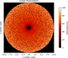 |
Fig. 2 Polarization map as a function of stellar radius for WR93b star with rotation rate |

3 Rotational effect
In this section, we demonstrate the effect of rotation on the polarization of scattered light. We conduct simulations for various values of  . The obtained polarization distribution in the
  plane by MCRT simulation is shown in Fig. 2. The results from comparing the single-scattering model (Eq. (5)), the single-scattering model with attenuation (Eq. (7)), and the multiple-scattering model with MCRT code are displayed in Fig. 3. These results show that the three models agree reasonably well up to an angular velocity of
  of the critical value. However, as the rotation increases beyond this point, there are noticeable deviations in the polarization induced by multiple-scattering compared to the single-scattering model.
Upon closer examination of the polarization data, it becomes evident that the impact of multiple-scattering is particularly pronounced at inclination angles of 40 and  . The degree of polarization experiences a significant increase at
  , followed by a sharp decrease at
  , as is shown in Fig. 4. Similar results were obtained by Wood et al. (1996b); Halonen & Jones (2013), in which the polarization peaked at an inclination lower than
  .
.
Figure 5 illustrates the effect of rotational velocity on polarization for an edge-on view. The graph demonstrates an increase in polarization as the rotation rate  increases, reaching a peak around
  , similar to the result in Fig. 4. Moreover, the observed upper limit of polarization (Stevance et al. 2018) for both WR93b (
  ) and WR102 (
  ) indicates a rotation rate of
  , corresponding to rotational velocities of less than
  and
and  , respectively. By using the formula
  to calculate the specific angular momentum, we find that
  . We note that these values of angular momentum are comparable to the ones obtained by Stevance et al. (2018) and Abdellaoui et al. (2022). For the scaled polarization by
  , we can observe that the relative rotation rates are
  and
and  , which correspond to a rotational velocity of
  , and
, and  , for WR93b and WR102, respectively.
According to the threshold set by MacFadyen & Woosley (1999), for a star to collapse into a LGRB the angular momentum, j, must exceed  . As our calculated values exceed this threshold, it can be inferred that these WR stars are potential candidates for LGRB.
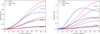 |
Fig. 3 Polarization as a function of inclination for single-scattering model (dotted red lines), single-scattering model with attenuation (dash-dotted black lines), and multiple-scattering model (full blue lines) of stars WR93b (left panel) and WR102 (right panel) computed for a fixed mass-loss rate as it is given in Table 1. |
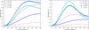 |
Fig. 4 Polarization as a function of inclination for the multiple-scattering model of stars WR93b (left panel) and WR102 (right panel) with different rotation rates, labeled in the panels. |
4 Mass-loss effect
Various factors influence the polarization properties of WR stars, and one important factor is the mass-loss rate. The mass-loss rate of a WR star determines the optical depth of its stellar wind, which affects the polarization of the scattered light.
To better understand this relationship, we examined a plot that shows the polarization as a function of inclination for different values of the mass-loss rate. We found that as the mass-loss rate increases, the degree of polarization also increases (see Fig. 6). This phenomenon occurs because higher mass-loss rates result in more scattering particles in the stellar wind, leading to higher polarization.
Therefore, the mass-loss rate plays a significant role in determining the polarization properties of WR stars. By understanding and studying this relationship, we can gain valuable insights into the physical processes occurring in these stars and further our understanding of their evolution and characteristics.
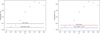 |
Fig. 5 Polarization as a function of rotation, |


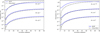 |
Fig. 6 Comparison of polarization from the multiple-scattering model (MCRT simulation, full blue lines) and single-scattering (Sing+Atten) model with attenuation (dash-dotted black lines) as a function of inclination for WR93 (left panel) and WR102 (right panel). The blue and black lines are labeled with the mass-loss rates in units of |

5 Conclusion
Our study has examined the polarization resulting from electron scattering in a rotating stellar wind. We have looked at cases in which a point source of radiation illuminated the wind. We have studied how different parameters affected the polarization behavior when there was only scattering or scattering with absorption.
We found that the polarization strongly depends on the viewing angle for all models. Interestingly, our simulations revealed that multiple-scattering had a significant impact on the polarization compared to what would be predicted by analytical models assuming single-scattering.
For cases with shallow optical depths, our simulations were consistent with the  dependence of polarization described by Brown & McLean (1977). However, we observed that many of our models exhibited a peak at lower inclination angles for a high optical depth.
Our study provides insights into the complex polarization behavior in stellar winds and highlights the importance of considering multiple-scattering effects when interpreting observations. The obtained polarization is comparable to previous calculations, and the limit for a star to potentially produce a LGRB is satisfied, with the angular momentum that could be greater than  . These findings suggest that WR stars like WR93b and WR102 could indeed be the progenitors of LGRBs. Therefore, external factors such as magnetic fields, interactions with binary systems, or mass loss may significantly impact their ultimate fate. Further research involving spectropolarimetry and sophisticated modeling is crucial to better understand the role of these stars in LGRB progenitor populations.
In this study, we have applied the density model formulated by Dwarkadas & Owocki (2002), which originates from the gravity darkening theorem introduced by von Zeipel (1924). A more accurate description of gravity darkening has been developed for fast-rotating stars by Espinosa Lara & Rieutord (2011); the von Zeipel model remains a practical and widely used approximation for exploring the effects of rotation on stellar winds. For stars with rapid rotation, the more accurate description results in a reduced temperature ratio between poles and the equator, consequently causing a lower ratio of mass-loss rates in these regions. This lower mass-loss ratio leads to a slightly lower polarization than what is predicted here.
Acknowledgments
The authors thank Prof. R. Ignace and Prof. Stan Owocki for the useful discussion. We gratefully acknowledge support from the Grant Agency of the Czech Republic (GAČR 25-15910S). The Astronomical Institute of the Czech Academy of Sciences in Ondřejov is supported by the project RVO:67985815.Computational resources were provided by the e-INFRA CZ project (ID:90254), supported by the Ministry of Education, Youth and Sports of the Czech Republic.
References
- Abdellaoui, S., Krtička, J., & Kurfürst, P. 2022, A&A, 658, A46 [NASA ADS] [CrossRef] [EDP Sciences] [Google Scholar]
- Brown, J. C., & Fox, G. K. 1989, ApJ, 347, 468 [Google Scholar]
- Brown, J. C., & McLean, I. S. 1977, A&A, 57, 141 [NASA ADS] [Google Scholar]
- Brown, J. C., Carlaw, V. A., & Cassinelli, J. P. 1989, ApJ, 344, 341 [Google Scholar]
- Cassinelli, J. P., Nordsieck, K. H., & Murison, M. A. 1987, ApJ, 317, 290 [NASA ADS] [CrossRef] [Google Scholar]
- Chandrasekhar, S. 1950, Radiative Transfer (Dover Publications) [Google Scholar]
- Chiosi, C., Nasi, E., & Bertelli, G. 1979, A&A, 74, 62 [NASA ADS] [Google Scholar]
- Code, A. D., & Whitney, B. A. 1995, ApJ, 441, 400 [Google Scholar]
- Collins, G. W. II 1989, The Fundamentals of Stellar Astrophysics (W. H. Freeman & Co.) [Google Scholar]
- Conti, P. S. 1975, Mem. Soc. Roy. Sci. Liege, 9, 193 [Google Scholar]
- Crowther, P. A., Hillier, D. J., & Smith, L. J. 1995, A&A, 293, 172 [NASA ADS] [Google Scholar]
- Dessart, L., Hillier, D. J., Yoon, S.-C., Waldman, R., & Livne, E. 2017, A&A, 603, A51 [NASA ADS] [CrossRef] [EDP Sciences] [Google Scholar]
- Dwarkadas, V. V., & Owocki, S. P. 2002, ApJ, 581, 1337 [NASA ADS] [CrossRef] [Google Scholar]
- Espinosa Lara, F., & Rieutord, M. 2011, A&A, 533, A43 [NASA ADS] [CrossRef] [EDP Sciences] [Google Scholar]
- Friend, D. B., & Cassinelli, J. P. 1986, ApJ, 303, 292 [Google Scholar]
- Gormaz-Matamala, A. C., Cuadra, J., Ekström, S., et al. 2024, A&A, 687, A290 [NASA ADS] [CrossRef] [EDP Sciences] [Google Scholar]
- Gräfener, G., Vink, J. S., Harries, T. J., & Langer, N. 2012, A&A, 547, A83 [NASA ADS] [CrossRef] [EDP Sciences] [Google Scholar]
- Gräfener, G., Owocki, S. P., Grassitelli, L., & Langer, N. 2017, A&A, 608, A34 [NASA ADS] [CrossRef] [EDP Sciences] [Google Scholar]
- Grassitelli, L., Langer, N., Grin, N. J., et al. 2018, A&A, 614, A86 [NASA ADS] [CrossRef] [EDP Sciences] [Google Scholar]
- Groh, J. H., Meynet, G., Georgy, C., & Ekström, S. 2013, A&A, 558, A131 [NASA ADS] [CrossRef] [EDP Sciences] [Google Scholar]
- Halonen, R. J., & Jones, C. E. 2013, ApJ, 765, 17 [Google Scholar]
- Hamann, W. R., Gräfener, G., & Liermann, A. 2006, A&A, 457, 1015 [NASA ADS] [CrossRef] [EDP Sciences] [Google Scholar]
- Hoffman, J. L., Whitney, B. A., & Nordsieck, K. H. 2003, ApJ, 598, 572 [Google Scholar]
- Kurfürst, P., Pejcha, O., & Krtička, J. 2020, A&A, 642, A214 [NASA ADS] [CrossRef] [EDP Sciences] [Google Scholar]
- Lamers, H. J. G. L. M., & Cassinelli, J. P. 1999, Introduction to Stellar Winds (Cambridge University Press), 452 [CrossRef] [Google Scholar]
- MacFadyen, A. I., & Woosley, S. E. 1999, ApJ, 524, 262 [NASA ADS] [CrossRef] [Google Scholar]
- McLean, I. S. 1979, MNRAS, 186, 265 [NASA ADS] [Google Scholar]
- Nugis, T., & Lamers, H. J. G. L. M. 2002, A&A, 389, 162 [EDP Sciences] [Google Scholar]
- Owocki, S. P., Cranmer, S. R., & Gayley, K. G. 1996, ApJ, 472, L115 [Google Scholar]
- Peest, C., Camps, P., Stalevski, M., Baes, M., & Siebenmorgen, R. 2017, A&A, 601, A92 [NASA ADS] [CrossRef] [EDP Sciences] [Google Scholar]
- Petrenz, P., & Puls, J. 2000, A&A, 358, 956 [NASA ADS] [Google Scholar]
- Robitaille, T. P. 2011, A&A, 536, A79 [NASA ADS] [CrossRef] [EDP Sciences] [Google Scholar]
- Sander, A., Hamann, W. R., & Todt, H. 2012, A&A, 540, A144 [NASA ADS] [CrossRef] [EDP Sciences] [Google Scholar]
- Schootemeijer, A., Shenar, T., Langer, N., et al. 2024, A&A, 689, A157 [NASA ADS] [CrossRef] [EDP Sciences] [Google Scholar]
- Shenar, T., Gilkis, A., Vink, J. S., Sana, H., & Sander, A. A. C. 2020, A&A, 634, A79 [NASA ADS] [CrossRef] [EDP Sciences] [Google Scholar]
- Stevance, H. F., Ignace, R., Crowther, P. A., et al. 2018, MNRAS, 479, 4535 [NASA ADS] [CrossRef] [Google Scholar]
- Townsend, R. 2012, in Stellar Polarimetry: from Birth to Death, eds. J. L. Hoffman, J. Bjorkman, & B. Whitney, American Institute of Physics Conference Series, 1429, 278 [Google Scholar]
- Tramper, F., Straal, S. M., Sanyal, D., et al. 2015, A&A, 581, A110 [NASA ADS] [CrossRef] [EDP Sciences] [Google Scholar]
- Vanbeveren, D., Van Bever, J., & Belkus, H. 2007, ApJ, 662, L107 [NASA ADS] [CrossRef] [Google Scholar]
- Vink, J. S., & de Koter, A. 2005, A&A, 442, 587 [NASA ADS] [CrossRef] [EDP Sciences] [Google Scholar]
- von Zeipel, H. 1924, MNRAS, 84, 665 [NASA ADS] [CrossRef] [Google Scholar]
- Wood, K., Bjorkman, J. E., Whitney, B., & Code, A. 1996a, ApJ, 461, 847 [Google Scholar]
- Wood, K., Bjorkman, J. E., Whitney, B. A., & Code, A. D. 1996b, ApJ, 461, 828 [NASA ADS] [CrossRef] [Google Scholar]
- Woosley, S. E. 1993, ApJ, 405, 273 [Google Scholar]
Hyperion is published under an open-source license at http://www.hyperion-rt.org
All Tables
All Figures
|
Fig. 1 Wind density contours for the rotation rates |
| In the text | |
|
Fig. 2 Polarization map as a function of stellar radius for WR93b star with rotation rate |
| In the text | |
|
Fig. 3 Polarization as a function of inclination for single-scattering model (dotted red lines), single-scattering model with attenuation (dash-dotted black lines), and multiple-scattering model (full blue lines) of stars WR93b (left panel) and WR102 (right panel) computed for a fixed mass-loss rate as it is given in Table 1. |
| In the text | |
|
Fig. 4 Polarization as a function of inclination for the multiple-scattering model of stars WR93b (left panel) and WR102 (right panel) with different rotation rates, labeled in the panels. |
| In the text | |
|
Fig. 5 Polarization as a function of rotation, |
| In the text | |
|
Fig. 6 Comparison of polarization from the multiple-scattering model (MCRT simulation, full blue lines) and single-scattering (Sing+Atten) model with attenuation (dash-dotted black lines) as a function of inclination for WR93 (left panel) and WR102 (right panel). The blue and black lines are labeled with the mass-loss rates in units of |
| In the text | |
Current usage metrics show cumulative count of Article Views (full-text article views including HTML views, PDF and ePub downloads, according to the available data) and Abstracts Views on Vision4Press platform.
Data correspond to usage on the plateform after 2015. The current usage metrics is available 48-96 hours after online publication and is updated daily on week days.
Initial download of the metrics may take a while.