| Issue |
A&A
Volume 657, January 2022
|
|
|---|---|---|
| Article Number | A55 | |
| Number of page(s) | 8 | |
| Section | Atomic, molecular, and nuclear data | |
| DOI | https://doi.org/10.1051/0004-6361/202142434 | |
| Published online | 06 January 2022 | |
Deexcitation rate coefficients of C3 by collision with H2 at low temperatures★
1
Departamento de Física, Facultad de Ciencias Físicas y Matemáticas, Universidad de Chile,
Santiago
837.0415, Chile
2
Instituto de Ciencias Químicas Aplicadas, Facultad de Ingeniería, Universidad Autónoma de Chile,
Av. Pedro de Valdivia 425,
7500912
Providencia,
Santiago, Chile
e-mail: otoniel.denis@uautonoma.cl
3
Departamento de Física, Facultad de Ciencias, Universidad de Chile,
Casilla 653,
Santiago
7800024,
Santiago, Chile
4
Centro para el Desarrollo de la Nanociencia y la Nanotecnología (CEDENNA),
Avda. Ecuador 3493,
Santiago
9170124, Chile
e-mail: cardena@uchile.cl
Received:
14
October
2021
Accepted:
10
November
2021
Context. An accurate analysis of the physical-chemical conditions in the regions of the interstellar medium in which C3 is observed requires knowing the collisional rate coefficients of this molecule with He, H2, electrons, and H.
Aims. The main goals of this study are to present the first potential energy surface for the C3 +H2 complex, to study the dynamics of the system, and to report a set of rate coefficients at low temperature for the lower rotational states of C3 with para- and ortho-H2.
Methods. A large grid of ab initio energies was computed at the explicitly correlated coupled-cluster with single-, double-, and perturbative triple-excitation level of theory, together with the augmented correlation-consistent quadruple zeta basis set (CCSD(T)-F12a/aug-cc-pVQZ). This grid of energies was fit to an analytical function. The potential energy surface was employed in close-coupling calculations at low collisional energies.
Results. We present a high-level four-dimensional potential energy surface (PES) for studying the collision of C3 with H2. The global minimum of the surface is found in the linear HH-CCC configuration. Rotational deexcitation state-to-state cross sections of C3 by collision with para- and ortho-H2 are computed. Furthermore, a reduced two-dimensional surface is developed by averaging the surface over the orientation of H2. The cross sections for the collision with para-H2 using this approximation and those from the four-dimensional PES agree excellently. Finally, a set of rotational rate coefficients for the collision of C3 with para- and ortho-H2 at low temperatures are reported.
Key words: astrochemistry / molecular data / molecular processes / scattering / ISM: molecules
Tables 5 and 6 are only available at the CDS via anonymous ftp to cdsarc.u-strasbg.fr (130.79.128.5) or via http://cdsarc.u-strasbg.fr/viz-bin/cat/J/A+A/657/A55
© ESO 2022
1 Introduction
Small carbon chains, such as C2, C3, and C5, have been observed in several regions of the interstellar medium (ISM) (Souza & Lutz 1977; Giesen et al. 2020; Maier et al. 2001; Hinkle et al. 1988; Bernath et al. 1989). They are expected to be the building blocks of more complex organic molecules that could explain the origin of life. Furthermore, these molecules could form larger chains, such as polycyclic aromatic hydrocarbon (PAH) and fullerene, which are candidates for explaining some of the diffuse interstellar bands (DIBs) (Omont et al. 2019).
In typical molecular clouds, the density and temperature are low (102–104 cm−3 and 10–15 K). Therefore, the rotational population of the molecules detected cannot be described by a Boltzmann distribution. In these cases, an accurate analysis of the physical-chemical conditions of these regions should be made using nonlocal thermal equilibrium (non-LTE) models. These models require knowing the Einstein coefficients and state-to-state rate coefficients of the observed molecules with the most common colliders in the ISM. However, the rate coefficients for the collision with H2, He, H, and e are not always available.
The C3 molecule has no dipole moment, but it can be detected through its rovibrational transitions. Even in cases like this, knowing the rotational state-to-state rate coefficients is valuable. For example, due to the absence of specific rotational rate coefficients for C3, the molecular abundance and excitation temperatures of this species in Sgr B2 and IRC+10216 were estimated by Cernicharo et al. (2000) using the rotational rates for OCS with H2 within a given vibrational level, while those between the ground and bending states were the same rotational rates divided by 10. Furthermore, due to the lack of data for C3 at that moment, Roueff et al. (2002) assumed the collisional rates to be proportional to the radiative line strengths in the analysis of the observation of C3 in the translucent molecular cloud toward HD 210121, and concluded that it will be essential to understand the inelastic collisions with C3 better.
The interaction of C3 with He has been widely studied. Abdallah et al. (2008) computed a PES at the coupled-cluster with single-, double-, and perturbativetriple-excitation level of theory (CCSD(T)) and reported the rate coefficients at low temperature, below 15 K, considering C3 as a rigid rotor. More recently, Smith et al. (2014) presented a new PES calculated with the CCSDT(Q) method, using the rigid-monomer approximation. They extended the set of rate coefficients up to 100 K. Two PESs at the CCSD(T) and CCSD(T)-F12 level considering the bending angle of C3 in the C3 + He complex were also developed (Denis-Alpizar et al. 2014; Al Mogren et al. 2014). Furthermore, the inclusion of the bending of C3 in the close coupling calculations was investigated by Stoecklin et al. (2015). In this work, the cross sections computed using the rigid-rotor approximation and including the bending motion showed differences only for collisions energies higher than the bending frequency of C3.
After the first studies of the collision C3 with He, Schmidt et al. (2014) reported the detection of this molecule toward HD 169454. In the analysis of the data, these author employed the same approximation as Roueff et al. (2002) and also included the rates for C3 + He (Abdallah et al. 2008), scaled to represent the collision with H2, and the deexcitations from higher levels were fixed at values from rotational state j = 10 in the RADEX code (Van der Tak et al. 2007). The model using the new rates showed that a higher destruction rate is required to fit the observed column densities well. These authors also proposed that detailed research of collisional rates is necessary before the physical conditions of the molecular gas can be deduced in detail from the C3 column densities.
The collision of C3 with atomic hydrogen was studied recently by Chhabra and Dhilip Kumar (Chhabra & Dhilip Kumar 2019). These authors build a two-dimensional PES for the ground states of C3 + H at the MRCI level and reported the rate coefficients up to 100 K. Even if the collision of C3 with H2 is nonreactive at low temperature (Mebel et al. 1998; Costes et al. 2006), no collisional rate coefficients have been reported so far. The rates for C3 + para-H2(j = 0) can be estimated from those with He (Schöier et al. 2005). However, it has been shown that this approximation is not valid in all cases, and in general, it is not valid for collisions with ortho-H2 (Kłos & Lique 2008; Vera et al. 2014; Denis-Alpizar et al. 2018). Therefore, the collision of C3 with H2 deserves to be investigated.
The main goals of this study are to present the first potential energy surface for the C3 + H2 complex, to study the dynamics of the system, and to report a set of rate coefficients at low temperature for the lower rotational states of C3 with para- and ortho-H2. This paper is organized as follows. In the next section, we present the methods we employed, and the results are discussed in Sect. 3. Finally, the main conclusions are summarized in Sect. 3.2.
2 Calculations
2.1 Ab initio calculations
The coordinates we employed to study the C3 + H2 complex are shown in Fig. 1. R connects thecenters of mass of the H2 and C3 molecules, and θ1, θ2, and φ describe the angular orientations of both systems. C3 and H2 are considered rigid rotors in this work. The bond length of H2 was taken as the vibrationally averaged value in the rovibrational ground state rH −H = 0.76664 Å (Jankowski & Szalewicz 1998), while the distances between C=C were set to the equilibrium value of the C3 molecule, rC −C = 1.277 Å (Van Orden & Saykally 1998).
Table 1 shows the interaction energies computed using different methods and basis sets. The energies at the completed-basis-set (CBS) limit were estimated with the two-point extrapolation formula (Halkier et al. 1999), 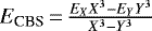 , where X = 5 and Y = 4 are the cardinality of the aug-cc-pV5Z, and aug-cc-pVQZ basis sets from CCSD(T) calculations. The CCSD(T)-F12a/aug-cc-pVQZ method gives energies close to the CBS limit at a relatively low computational cost. Therefore, all ab initio calculations were performed with this method as implemented in MOLPRO package (Werner et al. 2012). The size inconsistency of the CCSD(T)-F12a method was corrected by shifting up the ab initio interaction energies to make it vanish at R = 200 Å (Lique et al. 2010). The basis set superposition error was corrected using the counterpoise procedure of Boys and Bernardi (Boys & Bernardi 1970).
In total, 38 870 ab initio energies were computed. The radial coordinate R includes 23 values from 1.7 Å to 10.0 Å, while θ1 and θ2 vary from 0° to 180° in steps of 15°. The azimuthal angle φ varies in steps of 20° in the [0, 180]° interval.
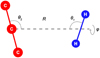 |
Fig. 1 Internal coordinates used to describe the C3 + H2 system. The azimuthal angle φ is undefined when either θ1 or θ2 is equal to 0° or 180°. |
2.2 Analytical four-dimensional surface
The grid of ab initio energies was fit following the same procedure as was recently used to study the HCO+ + H2 complex (Denis-Alpizar et al. 2020). The analytical function employed has the form
 (1)
(1)
where the angular part is represented by a product of normalized associated Legendre polynomials and a cosine function. The molecules H2 and C3 have a center of symmetry; thus, l1 and l2 are restricted to even values (Nasri et al. 2015). For each value of R, the ab initio energies were fit using a least-squares method. Each coefficient  was then fit using the reproducing kernel Hilbert space (RKHS) procedure (Ho & Rabitz 1996),
 (2)
(2)
where N is the number of radial points of thegrid (Rk). The q2,4(R, Rk) is the one-dimensional kernel, defined as
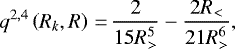 (3)
(3)
R> and R< are the greater and lower value between the Rk and R. The  coefficients were found by solving the system of linear equations
 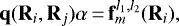 where i and j label the differentradial geometrical configurations of the grid.
Interaction energy (in cm−1) of H2 with C3 at the fixed angles (θ1 = 0° and θ2 = 90°) for several values of R using different methods and basis sets (the aug-cc-pVXZ basis sets are represented as AVXZ).
2.3 Averaged surface
The use of a two-dimensional PES averaged over the orientation of H2 to study the collision of a molecule with para-H2(j = 0) reduces computational cost in ab initio and dynamics calculations. This approximation has shown a reasonable agreement in the determination of the rate coefficients with those computed using the four-dimensional surface in several studies, for instance, SiS (Lique et al. 2008), HNC (Dumouchel et al. 2011), HCO+ (Massó & Wiesenfeld 2014), and CF+ (Desrousseaux et al. 2019). This is justified because in the dynamics of the collision with para-H2(j = 0), the coupling matrix elements are nonzero if l1 = 0 (see Eq. (9) in Green 1975).
The four-dimensional PES can be averaged as
 (4)
(4)
and if only the first rotational state of para-H2 is considered, the rotational angular momentum of H2, j1, and its projection on the intermolecular axis, k, are equal tozero. This averaged PES can be obtained numerically by quadrature. However, this would require knowing the four-dimensional PES, and one of the goals of this approximation is to reduce the calculation times in the development of the PES. It has been shown that considering three orientations of H2 is a good approximation to determine the averaged PES (Najar et al. 2014), and this is what we used here. The averaged energies were then computed as
![\begin{align*} &E_{\mathrm{av}}\left(R, \theta_{2}\right)\,{=}\,\frac{1}{3}\left\{E\left(R, \theta_{1}\,{=}\,0^{\circ}, \theta_{2}, \varphi\,{=}\,0^{\circ}\right)\right. \nonumber\\[3pt] &\left.+E\left(R, \theta_{1}\,{=}\,90^{\circ}, \theta_{2}, \varphi\,{=}\,0^{\circ}\right)+E\left(R, \theta_{1}\,{=}\,90^{\circ}, \theta_{2}, \varphi\,{=}\,90^{\circ}\right)\right\}.\end{align*}](/articles/aa/full_html/2022/01/aa42434-21/aa42434-21-eq10.png) (5)
(5)
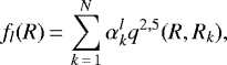
A grid of energies from Eq. (5), in the same intervals for R and θ1 as were used for the four-dimensional PES, was then fit to the analytical expression
 (6)
(6)
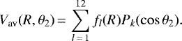
For each value of R, the fl (R) coefficients were computed using a least-squares procedure. The fl(R) were then fit using the RKHS method, such as
 (7)
(7)
where q2,5(R, Rk) is the one-dimensional kernel (Ho & Rabitz 1996), defined as
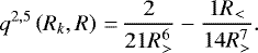 (8)
(8)
The subscript k corresponds to the k–ith radial point of the grid, and N is the number of R. R> and R< are the greater and lower value between the Rk and R. The  coefficients were obtained by solving the linear equations system
 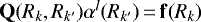 , where
 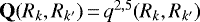 , and k and k′ label the geometrical configurations of the grid.
2.4 Scattering calculations
The four-dimensional PES was included in the Didimat code (Guillon et al. 2008) to study the collision of C3 with para-H2 and ortho-H2. This code solves the close-coupling equations in the space-fixed frame. The log-derivative propagator (Manolopoulos 1988) was employed starting from 3 a0. The minimum value of the maximum propagation distance was set to 60 a0 and extended automatically. At each collision energy, the convergence of the quenching cross sections was checked as a function of the total angular momentum and maximum propagation distance. The rotational constants of H2 and C3 we used are  cm−1 (Huber & Herzberg 1979) and
  cm−1 (Van Orden & Saykally 1998). The inclusion of 18 rotational states of C3 in the basis for the close-coupling calculation was enough to reach convergence. Table 2 shows the deexcitation cross sections for the collision with para-H2 including one (
 ) and two (
 ) rotational states in the basis at the collisional energies of 10 and 100 cm−1. The cross sections with the two bases agree well at both energies. The average percent difference is lower than 4.2% at 10 cm−1 (this energy is in the region in which the resonances strongly affect the magnitude of the cross sections) and reduces to 2% at 100 cm−1. Therefore, only one rotational state of H2 was included in the basis to study the dynamics of the collision.
Furthermore, the averaged PES was employed to study the dynamics of the collision of C3 with para-H2(j = 0). In this case,the code for investigating the atom-molecule collision, Newmat (Stoecklin et al. 2002), was used. The close-coupling equations were solved in the space-fixed frame, and the log-derivative propagator was also employed (Manolopoulos 1988). The minimum value of the largest propagation distance was 50 a0 and was automatically extended. At each collisional energy, the convergence of the quenching cross section was checked as a function of the maximum intermolecular distance and the total angular momentum. In these calculations, 18 rotational states of C3 were also considered.
Finally,the state-to-state deexcitation rate coefficients ( ) were computed by the average of the rotational cross sections (
 ) over a Maxwell-Boltzmann distribution at a given temperature T, as
 (9)
(9)
where ji and jf are the initial and final rotational states of C3, Ec is the collisional energy, and kB is the Boltzmann constant.
Rotational deexcitation cross sections (in  ) of C3 by collision with para-H2 using one (
 ) and two (
 ) states of H2 in the dynamics calculations at collisional energies of 10 and 100 cm−1 for the lower transitions.
3 Results and discussion
3.1 Potential energy surface
The quality of the fit of the four-dimensional PES was checked by evaluating the root-mean-square deviation (RMSD) of the ab initio energies of the grid and the fitted values. For E ≤ 0 cm−1, the RMSD was 6.19 × 10⁻² cm−1. In the intervals 0 ≤ E ≤ 1000 cm−1, 1000 ≤ E ≤ 5000 cm−1, and 5000 ≤ E ≤ 10 000 cm−1, the RMSD were 0.155, 0.286, and 2.143 cm−1, respectively.
Furthermore, a set of 987ab initio energies (Eab) not employed in the fitting procedure was computed. The averaged percentage difference between these energies and those (Eana) computed with the analytical PES (100 × |(Eab − Eana)∕((Eab + Eana)∕2)) for Eab < 5000 cm−1 is lower than 2.6%, while in the 5000 ≤ Eab < 20 000 cm−1 interval, thisvalues is 2.1%. Figure 2A shows the computed energies and the ab initio energies at geometrical configurations outside the grid that was used in the fit, which confirms that the agreement is very good. This figure also gives an indication of the anisotropy of the interaction.
The long range of the PES is also analysed from the multipolar expansion. The interaction energy can be written as the sum of the electrostatic (Eelec), induction (Eind), and dispersion (Edisp) contributions, such as (Pullman 1978)
 (10)
(10)
 (11)
(11)
![\begin{eqnarray*} E_{\textrm{disp}} &=& \frac{3U_AU_B}{2(U_A+U_B)R^{6}}\left[\alpha^A\alpha^B+\frac{1}{3}\alpha^A(\alpha_{zz}^B - \alpha_{xx}^B)\left(\frac{3}{2}\cos^2\theta_2-\frac{1}{2}\right) \right. \nonumber\\ && \left. +\frac{1}{3}\alpha^B(\alpha_{zz}^A - \alpha_{xx}^A)\left(\frac{3}{2}\cos^2\theta_1-\frac{1}{2}\right)\right], \end{eqnarray*}](/articles/aa/full_html/2022/01/aa42434-21/aa42434-21-eq26.png)
where α = (2αxx + αzz)∕3 is a mean polarizability. Superscripts A and B denote the H2 and C3 molecules, respectively,and U is the ionization energy (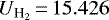 eV and
  eV) (Johnson 2002). The computed molecular properties of C3 and H2 are listed in Table 3. Figure 2B shows the excellent agreement between the analytical multipolar energies and those from our PES. This makes this surface suitable for studying cold molecular collisions.
Figure 3 shows the contour plot of the analytical PES at several geometrical configurations. A strong dependence of the energies on the angular orientation is shown in this figure. The global minimum of the surface, named − 135.64 cm−1, was found at the R = 4.76 Å, in the linearconfiguration H–H–C–C–C, see panel A and D. This well is around 5 times deeper than the one found in C3 + He (− 25.87 cm−1 Abdallah et al. 2008, − 25.54 cm−1 Zhang et al. 2009, − 31.29 cm−1 Zhang et al. 2009, − 26.73 cm−1 Denis-Alpizar et al. 2014 and − 27.91 cm−1 Al Mogren et al. 2014).
Figure 3 also shows apparent local minima; see panels B, C, E, and F. However, Fig. 4 shows a contour plot in which R relaxes from 3.0 to 5.0 Å for φ = 0° and θ1 = 90°. Only two secondary minima are observed in these figures: E = − 123.7 cm−1 at (θ1 = 69°, θ2 = 122°, φ = 0°) and at symmetric configuration; and E = − 103.4 cm−1 at (θ1 = 90°, θ2 = 90°, φ = 0°). A Fortran subroutine of this PES is available upon request to the authors or at the github link1.
We also evaluated an averaged two-dimensional PES using the energies from Eq. (5). Figure 5 shows a contour plot of this surface. The minimum of this surface, − 78.62 cm−1 was found at θ2 = 90°, and R = 3.6 Å. This value is also higher than the value for the collision with He, but at the same T configuration. Additionally, an averaged PES was computed from Eq. (4) using a Gauss-Chebyshev quadrature of 20 points for the integration over φ and a Gauss–Legendre quadrature with 20 points over θ1. This surfaceshows the same behavior as that of Fig. 5 (without visible differences). The minimum of this surface (− 78.70 cm−1) was found at the same geometrical configuration as the averaged PES shown in Fig. 5.
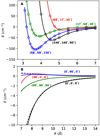 |
Fig. 2 Interaction energy along R of the C3 + H2 complex. Panel A: energies computed using the four-dimensional PES (solid lines) and from ab initio calculations (points) at several angular configuration (θ1, θ2, φ) of C3 and H2 that are notincluded in the grid used for the fit. Panel B: energies computed from the PES (solid lines) and analytical multipolar expansion (dashed line) at several angular configuration. |
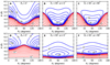 |
Fig. 3 Contour plot of the PES for the C3 + H2 complex at several geometrical configurations. Negative energies are represented as blue lines in steps 20 cm−1. Positive energies (red lines) are logarithmically spaced between 1 cm−1 and 104 cm−1. |
Molecular properties of C3 and H2 calculated at the CCSD(T)/aug-cc-pV5Z level using the finite-field method of Cohen and Roothaan1.
3.2 Dynamics
The four-dimensional PES presented in the previous section was employed in close-coupling calculations for collision energies from 10−2 up to 300 cm−1. These calculations were performed for energies higher than the bending frequencies of C3 (ω = 63 cm−1). In the study of the dynamics of C3 in collision with He including the bending motion, the rotational deexcitation cross sections in the ground-vibrational state of the triatomic system agreed very well with those computed using the rigid-rotor approximation for energies lower than ω (Stoecklin et al. 2015). With increasing collisional energy, this good agreement between the two sets of cross sections decreases. For example, for the transition 4 → 0 at 200 cm−1, the rigid-rotor approximation overestimated the cross section by 20% (Denis-Alpizar 2014). This difference is also observed in the rate coefficients. At 50 K, the rates computed by Stoecklin et al. (2015) considering the molecule as a rigid rotor and including the bending motion of C3 showed a percent difference of 21% (averaged over all deexcitation transitions for j ≤ 10). This percent difference increases with increasing temperature. Therefore, we expect that considering the monomers as rigid rotors is a reasonably good approximation for collisional energies up to 300 cm−1. In the case of C3 + H2, the PES is deeper than for C3+He, and the bending-rotation coupling could be stronger. The cross sections at high collisional energies should be considered with caution.
Figure 6 shows the rotational cross sections for the collision of C3 with para- and ortho-H2. The cross sections decrease with increasing collision energy and |Δj|. The typical shape and Feshbach resonances, associated with the formation of quasi-bound states due to the PES centrifugal barrier and as a result of the coupling between open and closed channels (Yazidi et al. 2014), can also be observed in this figure.
The cross sections for the collision with para-H2 from the averaged PES are also included in Fig. 6. These values agree very well with the cross sections computed using the four-dimensional PES. The use of a reduced PES has shown to be a reasonably good approximation for determining the rate coefficients in the study of the collision of other systems (SiS Lique et al. 2008, HNC Dumouchel et al. 2011, C2H Dagdigian 2018, CF+ Desrousseaux et al. 2019, N2H+ Balança et al. 2020, and HCO+ Denis-Alpizar et al. 2020). The C3 molecule is another case that shows that this is an attractive approximation for estimating the rate coefficients with para-H2 at reduced computational cost.
A set of rate coefficients for the lower rotational states of C3 (up to j = 20) for the collision with para- and ortho-H2 was determined from the computed cross sections at temperatures lower than 50 K. These rates are reported in Table 4 and in the supplementary material. The difference between the rates with para- and ortho-H2 is small. This behavior has recently been observed in the study of the collisions with H2 of several systems, for instance, C4H− (Balança et al. 2021), HCO+ (Denis-Alpizar et al. 2020), DCO+ (Denis-Alpizar et al. 2020), N2H+ (Balança et al. 2020), SH+ (Dagdigian 2019), CF+ (Desrousseaux et al. 2019), C3N− (Lara-Moreno et al. 2019), C6H− (Walker et al. 2017), HC3N (Wernli et al. 2007), and CN− (Kłos & Lique 2011). At low temperatures, this is associated with the effects of the long-range part of the interaction outweighing those of the short range (Balança et al. 2021).
Furthermore, the rates for the collision with He determined by Abdallah et al. (2008) that are available in the Basecol database (Dubernet et al. 2013) and the rates for the collision with H, computed from the excitation rates from Chaabra and Dhilip Kumar (Chhabra & Dhilip Kumar 2019) using the principle of detailed balance, are also included in Table 4. The rates for the collision with He are lower than those for the collision with para- and ortho-H2. The mass-scaling approximation for determining the rates for the collision with para-H2 from those with He was evaluated. The ratio of the rates with para-H2 and He is 1.40 at 5 K, 1.54 at 10 K, and 1.64 at 15 K. These values are close to the 1.4 scaling factor that is commonly employed (Schöier et al. 2005), but this ratio varies from 0.8 up to 2.4, and this approximation should be considered with cation for C3. In the case of the collision with H, our rates are also higher. Chhabra and Dhilip Kumar (Chhabra & Dhilip Kumar 2019) found that the rates for H were lower than those for He, and they associated this behavior with the different PES and colliders. Finally, we expect that the new rate coefficients reported here will be useful in determining the interstellar conditions in the regions in which this molecule has been detected.
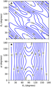 |
Fig. 4 Contour plot of the PES for the C3 + H2 complex. R is relaxed from 3.0 to 5.0 Å for φ = 0° (panel A) and θ2 = 90° (panel B). Inthe range [−125, 0] cm−1, the space between the lines is 15 cm−1 and 5 cm−1. |
 |
Fig. 5 Contour plot for the averaged PES of the C3 + H2 complexcomputed from Eq. (5). The space between blue lines is 20 cm−1 in the range [−70, 0] cm−1, and the red lines are logarithmically spaced between 1 cm−1 and 104 cm−1. |
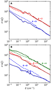 |
Fig. 6 Rotational deexcitations cross sections of C3 from the initial rotational state j = 4 (panel A) and j = 6 (panel B), incollision with para-H2 (solid lines), ortho-H2 (dashed lines), and para-H2 from averaged PES (dotted black lines). Rotational transitions of C3 are labeled ji → jf. |
Rotational deexcitation rate coefficients (×10−11 cm3 molecule−1 s−1) of C3 in collision with ortho-H2, and para-H2 at several temperatures.
4 Conclusions
We developed the first four-dimensional PES for the C3 -H2 complex. This surface was fit from a large grid of ab initio energies computed at the CCSD(T)-F12a/aug-cc-pVQZ level of theory. The global minimum of the surface was found in the linear CCC-HH configuration. This surface was employed in close-coupling calculations. The cross sections for the lower rotational states of C3 in collision with H2 were computed. Furthermore, an averaged PES over the orientation of H2 was used to study the relaxation of C3 with para-H2(j = 0). The cross sections using this surface and those computed with the four-dimensional PES were found to agree very well. Finally, we reported a set of rate coefficients for the lower rotational states of C3 with para- and ortho-H2 at low temperature.
Acknowledgements
Support from projects CONICYT/FONDECYT/ REGULAR/ Nos. 1200732 and 1181121 is gratefully acknowledged. This research was partially supported by the supercomputing infrastructure of the NLHPC (ECM-02). C.C. acknowledges Center for the Development of Nanoscience and Nanotechnology CEDENNA AFB180001
References
- Abdallah, D. B., Hammami, K., Najar, F., et al. 2008, ApJ, 686, 379 [NASA ADS] [CrossRef] [Google Scholar]
- Al Mogren, M. M., Denis-Alpizar, O., Abdallah, D. B., et al. 2014, J. Chem. Phys., 141, 044308 [NASA ADS] [CrossRef] [Google Scholar]
- Balança, C., Scribano, Y., Loreau, J., Lique, F., & Feautrier, N. 2020, MNRAS, 495, 2524 [Google Scholar]
- Balança, C., Quintas-Sánchez, E., Dawes, R., et al. 2021, MNRAS, 508, 1148 [CrossRef] [Google Scholar]
- Bernath, P. F., Hinkle, K. H., & Keady, J. J. 1989, Science, 244, 562 [NASA ADS] [CrossRef] [Google Scholar]
- Boys, S. F., & Bernardi, F. 1970, Mol. Phys., 19, 553 [NASA ADS] [CrossRef] [Google Scholar]
- Cernicharo, J., Goicoechea, J. R., & Caux, E. 2000, ApJ, 534, L199 [NASA ADS] [CrossRef] [Google Scholar]
- Chhabra, S., & Dhilip Kumar T. J. 2019, J. Phys. Chem. A, 123, 7296 [NASA ADS] [CrossRef] [Google Scholar]
- Cohen, H. D., & Roothaan, C. C. J. 1965, J. Chem. Phys., 43, S34 [NASA ADS] [CrossRef] [Google Scholar]
- Costes, M., Daugey, N., Naulin, C., et al. 2006, Faraday Discuss. Chem. Soc., 133, 157 [Google Scholar]
- Dagdigian, P. J. 2018, J. Chem. Phys., 148, 024304 [NASA ADS] [CrossRef] [Google Scholar]
- Dagdigian, P. J. 2019, MNRAS, 487, 3427 [Google Scholar]
- Denis-Alpizar, O. 2014, PhD thesis, Université de Bordeaux [Google Scholar]
- Denis-Alpizar, O., Stoecklin, T., & Halvick, P. 2014, J. Chem. Phys., 140, 084316 [NASA ADS] [CrossRef] [Google Scholar]
- Denis-Alpizar, O., Stoecklin, T., Guilloteau, S., & Dutrey, A. 2018, MNRAS, 478, 1811 [Google Scholar]
- Denis-Alpizar, O., Stoecklin, T., Dutrey, A., & Guilloteau, S. 2020, MNRAS, 497, 4276 [Google Scholar]
- Desrousseaux, B., Quintas-Sánchez, E., Dawes, R., & Lique, F. 2019, J. Phys. Chem. A, 123, 9637 [NASA ADS] [CrossRef] [Google Scholar]
- Dubernet, M.-L., Alexander, M. H., Ba, Y. A., et al. 2013, A&A, 553, A50 [NASA ADS] [CrossRef] [EDP Sciences] [Google Scholar]
- Dumouchel, F., Kłos, J., & Lique, F. 2011, Phys. Chem. Chem. Phys., 13, 8204 [NASA ADS] [CrossRef] [Google Scholar]
- Giesen, T. F., Mookerjea, B., Fuchs, G. W., et al. 2020, A&A, 633, A120 [NASA ADS] [CrossRef] [EDP Sciences] [Google Scholar]
- Green, S. 1975, J. Chem. Phys., 62, 2271 [Google Scholar]
- Guillon, G., Stoecklin, T., Voronin, A., & Halvick, P. 2008, J. Chem. Phys., 129, 104308 [NASA ADS] [CrossRef] [Google Scholar]
- Halkier, A., Klopper, W., Helgaker, T., Jorgensen, P., & Taylor, P. R. 1999, J. Chem. Phys., 111, 9157 [NASA ADS] [CrossRef] [Google Scholar]
- Hinkle, K. W., Keady, J. J., & Bernath, P. F. 1988, Science, 241, 1319 [NASA ADS] [CrossRef] [Google Scholar]
- Ho, T. S., & Rabitz, H. 1996, J. Phys. Chem., 104, 2584 [CrossRef] [Google Scholar]
- Huber, K. P., & Herzberg, G. 1979, Molecular Spectra and Molecular Structure. IV. Constants of Diatomic Molecules (New York: Van Nostrand Reinhold) [CrossRef] [Google Scholar]
- Jankowski, P., & Szalewicz, K. 1998, J. Chem. Phys., 108, 3554 [CrossRef] [Google Scholar]
- Johnson, R. 2002, Computational Chemistry Comparison and Benchmark Database, NIST Standard Reference Database 101 [Google Scholar]
- Kłos, J., & Lique, F. 2008, MNRAS, 390, 239 [CrossRef] [Google Scholar]
- Kłos, J., & Lique, F. 2011, MNRAS, 418, 271 [Google Scholar]
- Lara-Moreno, M., Stoecklin, T., & Halvick, P. 2019, MNRAS, 486, 414 [CrossRef] [Google Scholar]
- Lique, F., Toboła, R., Kłos, J., et al. 2008, A&A, 478, 567 [NASA ADS] [CrossRef] [EDP Sciences] [Google Scholar]
- Lique, F., Kłos, J., & Hochlaf, M. 2010, Phys. Chem. Chem. Phys., 12, 15672 [CrossRef] [Google Scholar]
- Maier, J. P., Lakin, N. M., Walker, G. A. H., & Bohlender, D. A. 2001, ApJ, 553, 267 [NASA ADS] [CrossRef] [Google Scholar]
- Manolopoulos,D. E. 1988, PhD thesis, University of Cambridge [Google Scholar]
- Massó, H., & Wiesenfeld, L. 2014, J. Chem. Phys., 141, 184301 [Google Scholar]
- Mebel, A., Jackson, W., Chang, A., & Lin, S. 1998, J. Am. Chem. Soc., 120, 5751 [CrossRef] [Google Scholar]
- Najar, F., Abdallah, D. B., Spielfiedel, A., et al. 2014, Chem. Phys. Lett., 614, 251 [NASA ADS] [CrossRef] [Google Scholar]
- Nasri, S., Ajili, Y., Jaidane, N.-E., et al. 2015, J. Chem. Phys., 142, 174301 [NASA ADS] [CrossRef] [Google Scholar]
- Omont, A., Bettinger, H. F., & Tönshoff, C. 2019, A&A, 625, A41 [NASA ADS] [CrossRef] [EDP Sciences] [Google Scholar]
- Pullman, B., ed. 1978, Intermolecular Interactions: From Diatomics to Biopolymers (New York: John Wiley & Sons) [Google Scholar]
- Roueff, E., Felenbok, P., Black, J., & Gry, C. 2002, A&A, 384, 629 [NASA ADS] [CrossRef] [EDP Sciences] [Google Scholar]
- Schmidt, M., Krełowski, J., Galazutdinov, G., et al. 2014, MNRAS, 441, 1134 [NASA ADS] [CrossRef] [Google Scholar]
- Schöier, F. L., van der Tak, F. F. S., van Dishoeck, E. F., & Black, J. H. 2005, A&A, 432, 369 [Google Scholar]
- Smith, D. G. A., Patkowski, K., Trinh, D., et al. 2014, J. Phys. Chem. A, 118, 6351 [CrossRef] [Google Scholar]
- Souza, S. P., & Lutz, B. L. 1977, ApJ, 216, L49 [Google Scholar]
- Stoecklin, T., Voronin, A., & Rayez, J. C. 2002, Phys. Rev. A, 66, 042703 [NASA ADS] [CrossRef] [Google Scholar]
- Stoecklin, T., Denis-Alpizar, O., & Halvick, P. 2015, MNRAS, 449, 3420 [NASA ADS] [CrossRef] [Google Scholar]
- Van der Tak, F., Black, J. H., Schöier, F., Jansen, D., & van Dishoeck, E. F. 2007, A&A, 468, 627 [NASA ADS] [CrossRef] [EDP Sciences] [Google Scholar]
- Van Orden, A., & Saykally, R. J. 1998, Chem. Rev., 98, 2313 [CrossRef] [Google Scholar]
- Vera, M. H., Kalugina, Y., Denis-Alpizar, O., Stoecklin, T., & Lique, F. 2014, J. Chem. Phys., 140, 224302 [CrossRef] [Google Scholar]
- Walker, K. M., Lique, F., Dumouchel, F., & Dawes, R. 2017, MNRAS, 466, 831 [Google Scholar]
- Werner, H.-J., Knowles, P. J., Knizia, G., Manby, F. R., & Schütz, M. 2012, WIREs Comput. Mol. Sci., 2, 242 [Google Scholar]
- Wernli, M., Wiesenfeld, L., Faure, A., & Valiron, P. 2007, A&A, 464, 1147 [NASA ADS] [CrossRef] [EDP Sciences] [Google Scholar]
- Yazidi, O., Ben Abdallah, D., & Lique, F. 2014, MNRAS, 441, 664 [NASA ADS] [CrossRef] [Google Scholar]
- Zhang, G., Zang, D., Sun, C., & Chen, D. 2009, Mol. Phys., 107, 1541 [NASA ADS] [CrossRef] [Google Scholar]
All Tables
Interaction energy (in cm−1) of H2 with C3 at the fixed angles (θ1 = 0° and θ2 = 90°) for several values of R using different methods and basis sets (the aug-cc-pVXZ basis sets are represented as AVXZ).
Rotational deexcitation cross sections (in ) of C3 by collision with para-H2 using one () and two () states of H2 in the dynamics calculations at collisional energies of 10 and 100 cm−1 for the lower transitions.
Molecular properties of C3 and H2 calculated at the CCSD(T)/aug-cc-pV5Z level using the finite-field method of Cohen and Roothaan1.
Rotational deexcitation rate coefficients (×10−11 cm3 molecule−1 s−1) of C3 in collision with ortho-H2, and para-H2 at several temperatures.
All Figures
|
Fig. 1 Internal coordinates used to describe the C3 + H2 system. The azimuthal angle φ is undefined when either θ1 or θ2 is equal to 0° or 180°. |
| In the text | |
|
Fig. 2 Interaction energy along R of the C3 + H2 complex. Panel A: energies computed using the four-dimensional PES (solid lines) and from ab initio calculations (points) at several angular configuration (θ1, θ2, φ) of C3 and H2 that are notincluded in the grid used for the fit. Panel B: energies computed from the PES (solid lines) and analytical multipolar expansion (dashed line) at several angular configuration. |
| In the text | |
|
Fig. 3 Contour plot of the PES for the C3 + H2 complex at several geometrical configurations. Negative energies are represented as blue lines in steps 20 cm−1. Positive energies (red lines) are logarithmically spaced between 1 cm−1 and 104 cm−1. |
| In the text | |
|
Fig. 4 Contour plot of the PES for the C3 + H2 complex. R is relaxed from 3.0 to 5.0 Å for φ = 0° (panel A) and θ2 = 90° (panel B). Inthe range [−125, 0] cm−1, the space between the lines is 15 cm−1 and 5 cm−1. |
| In the text | |
|
Fig. 5 Contour plot for the averaged PES of the C3 + H2 complexcomputed from Eq. (5). The space between blue lines is 20 cm−1 in the range [−70, 0] cm−1, and the red lines are logarithmically spaced between 1 cm−1 and 104 cm−1. |
| In the text | |
|
Fig. 6 Rotational deexcitations cross sections of C3 from the initial rotational state j = 4 (panel A) and j = 6 (panel B), incollision with para-H2 (solid lines), ortho-H2 (dashed lines), and para-H2 from averaged PES (dotted black lines). Rotational transitions of C3 are labeled ji → jf. |
| In the text | |
Current usage metrics show cumulative count of Article Views (full-text article views including HTML views, PDF and ePub downloads, according to the available data) and Abstracts Views on Vision4Press platform.
Data correspond to usage on the plateform after 2015. The current usage metrics is available 48-96 hours after online publication and is updated daily on week days.
Initial download of the metrics may take a while.