| Issue |
A&A
Volume 680, December 2023
|
|
|---|---|---|
| Article Number | A113 | |
| Number of page(s) | 4 | |
| Section | Atomic, molecular, and nuclear data | |
| DOI | https://doi.org/10.1051/0004-6361/202348272 | |
| Published online | 19 December 2023 | |
Rate coefficients for the rotational de-excitation of OCS by collision with He★
Instituto de Ciencias Aplicadas, Facultad de Ingeniería, Universidad Autónoma de Chile,
Av. Pedro de Valdivia 425,
7500912
Providencia,
Santiago,
Chile
e-mail: otoniel.denis@uautonoma.cl
Received:
13
October
2023
Accepted:
18
October
2023
Context. In typical molecular clouds, analyzing the physicochemical conditions with nonlocal thermodynamic equilibrium models requires knowledge of the collisional rate coefficients between the detected molecule and the most common colliders in the interstellar medium (ISM); for example H2, He, and H. The OCS molecule has been widely observed in the ISM. However, the collision data available for this species were calculated using a potential energy surface (PES) that shows differences with surfaces presented recently.
Aims. The main goal of this work is to report a new set of rate coefficients for the collision of OCS with He based on a new PES computed at a high level of theory.
Methods. We developed an analytical PES using a large set of ab initio energies calculated using the coupled cluster with single, double, and perturbative triple excitations (CCSD(T)) method at the completed basis set limit for the OCS+He complex. We used this surface in close-coupling calculations, and computed a new set of collisional rate coefficients for OCS and He.
Results. We compare the de-excitation rate coefficients with previously available data. Furthermore, we observe a |Δj| = 1 propensity rule. Finally, we report a set of rate coefficients for the lower 39 rotational states of OCS, which is the largest set determined to date for this collision.
Key words: astrochemistry / molecular data / molecular processes / scattering / ISM: molecules
Rotational de-excitation rate coefficients (Table 2) are available at the CDS via anonymous ftp to cdsarc.cds.unistra.fr (130.79.128.5) or via https://cdsarc.cds.unistra.fr/viz-bin/cat/J/A+A/680/A113
© The Authors 2023
 Open Access article, published by EDP Sciences, under the terms of the Creative Commons Attribution License (https://creativecommons.org/licenses/by/4.0), which permits unrestricted use, distribution, and reproduction in any medium, provided the original work is properly cited.
This article is published in open access under the Subscribe to Open model. Subscribe to A&A to support open access publication.
1 Introduction
Carbonyl sulfide (OCS) has been detected in galactic (Jefferts et al. 1971) and extragalactic (Mauersberger et al. 1995) sources. This species has been found in the interstellar medium (ISM) in both (Tsuge & Watanabe 2023) the gas phase (Goldsmith & Linke 1981) and on icy grains (Palumbo et al. 1995). Furthermore, the OCS molecule has been observed in a wide variety of interstellar objects (Goldsmith & Linke 1981; Matthews et al. 1987; Charnley et al. 2001; van der Tak et al. 2003; Drozdovskaya et al. 2018).
In typical molecular clouds, the density and temperature are low, and therefore a Boltzmann distribution cannot describe the rotational population of the observed molecule. In these cases, for example in regions with low density, the physicochemical conditions in molecular clouds should be analyzed using nonlocal thermodynamic equilibrium (non-LTE) models. Such models require knowledge of the Einstein coefficients and the state-to-state collisional rate coefficients of the observed species with the most common colliders in the ISM (e.g., H2, He, H and e−).
The interaction of OCS with He has been widely studied experimentally (Burns & Coy 1984; Broquier et al. 1986; Danielson et al. 1987; Higgins & Klemperer 1999; Ross & Willey 2005) and theoretically (Sadlej & Edwards 1993; Gianturco & Paesani 2000; Howson & Hutson 2001; Flower 2001; Paesani & Whaley 2004; Li & Ma 2012). Most of these works were motivated by the fact that OCS is a popular probe of microscopic superfluid effects in helium clusters and droplets (Oliaee et al. 2017). Therefore, studies of the collision of OCS with He and H2 in conditions of astrophysical interest have been limited. The only available set of rate coefficients for OCS+He is that reported by Flower (2001). However, the potential energy surface (PES) used in this latter work was computed at the MP4 level of theory by Higgins & Klemperer (1999), and shows discrepancies with more recent PESs. For example, the global minimum of this latter PES is −45.39 cm−1, while in contrast, more recent PESs are reported to show a deeper minimum; for example, the morphing surface of Howson & Hutson (2001) from ab initio energies at the CCSD(T)/aug-cc-pVTZ level (−50.2 cm−1), the surface of Paesani & Whaley (2004), which is also at the MP4 level of theory (−49.31 cm−1), the PES of Li & Ma (2012) at the CCSD(T)/aug-cc-pVQZ (−51.06 cm−1), and the surface of Wang et al. (2014) using the CCSD(T)/avqz+33221 method (−51.33 cm−1).
In the case of the collision with H2, although a new PES was presented recently (Liu et al. 2017), the only set of rate coefficients available was determined by Green & Chapman (1978) based on an electron gas PES for OCS-He. Furthermore, using the rates with He to reproduce those with H2 from a mass scaling law is a common procedure that could lead to significant uncertainties in the case of collisions with light hydrides, but is expected to be a reasonable approximation for relatively heavy molecules (Wernli et al. 2007; Urzúa-Leiva & Denis-Alpizar 2020).
The main goal of this work is to report a new set of rotational rate coefficients for OCS in collision with He based on a new PES computed at a high level of theory. The paper is organized as follows. The methods used for developing the PES and calculating the collisional rates are presented in the following section, and Sect. 4 discusses the results. Finally, the conclusions are summarized in Sect. S4.
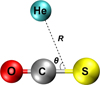 |
Fig. 1 Jacobi coordinates employed for studying the OCS+He complex. |
2 Methods
2.1 Ab initio calculations
In this work, the OCS molecule is considered as a linear rigid rotor with the interatomic distances fixed to the vibrationally averaged values of the O–C and C–S bond lengths in the ground state, rOC = 1.162839 Å and rCS = 1.55968 Å (Li & Ma 2012). The coordinates used for studying the interaction of OCS with He are shown in Fig. 1. R is the distance between the He atom and the center of mass of OCS, and θ is the angle between R and OCS, where θ = 0 corresponds to the linear He–OCS configuration.
The ab initio energies were calculated at the coupled cluster with single, double, and perturbative triple excitations (CCSD(T)) level of theory as implemented in the Molpro software (Werner et al. 2012). Table 1 shows the ab initio energies computed using different Dunning basis sets (Dunning 1989) and also employing the explicitly correlated CCSD(T) method (CCSD(T)-F12) at several geometrical configurations. Furthermore, the interaction energy was extrapolated at the completed basis set limit (CBS limit) using the two-point formula (Peterson et al. 1994), that is,  , where EX and Ey are the energies calculated at the respective cardinality of the basis set (e.g., X = 5 and Y = X − 1 = 4). As all the methods analyzed gave energies that were relatively far from the energy calculated at the CBS limit, either at one or several points, two grids of energies at the CCSSD(T)/aug-cc-pVQZ and CCSSD(T)/aug-cc-pVQZ level of theory were computed and used to obtain a grid at the CBS limit.
In all ab initio calculations, the basis set superposition error was corrected using the counterpoise procedure of Boys & Bernardi (1970). Each grid of energies includes 32 values of R between 2.0 and 20 Å, and 19 values of θ between 0° and 180° in steps of 10°.
2.2 Analytical potential energy surface
The grid of energies at the CBS limit was fitted to an analytical function where the angular part was represented in Legendre polynomials, as
 (1)
(1)
where the coefficients Cl(R) were computed using the weighted linear least square method at each fixed value of R. A weight depending on the energy  was applied. Subsequently, the coefficients Cl(R) were obtained by employing the reproducing kernel Hilbert space method (Ho & Rabitz 1996), as
 (2)
(2)
where N is the number of the radial grid, and Rk is the kth radial coordinate. The one-dimensional radial kernel is (Ho & Rabitz 1996)
 (3)
(3)
where the R> and R< are respectively the greater and the smaller between R and the radial coordinate of the grid Rk.
The  coefficients are found by solving the linear system Cl(R)= αlq(Ri, Rj), where i and j label the different radial configuration of the grid. The q2,5(Rk, R) kernel ensures the correct large range dependence R−6 (Soldán & Hutson 2000).
Ab initio energies of the OCS+He complex at several geometrical configurations computed using different methods and basis sets.
2.3 Inelastic scattering
The scattering of OCS with He was studied using the Newmat code (Stoecklin et al. 2002). This code solves the close coupling equation in the space-fixed frame. The log-derivative propagator (Manolopoulos 1988) was used from R = 3.7 a0 (1.96 Å), and the minimum value of maximum propagation distance was set to 40 a0 (21.17 Å) and extended automatically by the code up to 50.03 a0 (26.47 Å) at the lowest energies.
The rotational constant of OCS used in this work was Be = 0.20286 cm−1 (Herzberg 1966). Sixty-four rotational states of OCS were included in the bases. At each collisional energy (Ec), the convergence of the quenching cross-sections was checked as a function of total angular momentum (J). The maximum of J required to reach convergence at Ec = 500 cm−1 was 65.
The de-excitation rate coefficients of OCS by He at a given temperature (T) from an initial rotational state ji to a final rotational state  were computed as the average of the cross-sections
  over a Maxwell-Boltzmann distribution,
 (4)
(4)
where µ is the reduced mass of the system and kB is the Boltzmann constant.
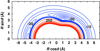 |
Fig. 2 Contour plot of the PES of the OCS+He complex. Positive energies (≥50 cm−1) are shown as red contour lines in steps of 200 cm−1, and negative (≤0 cm−1) contour lines (blue) are equally spaced in steps of 5 cm−1. |
3 Results and discussion
We verified the quality of the PES using the root means square deviation (RMSD) of the computed ab initio energies and the analytical values. For negative energies, the RMSD is 0.002 cm−1; for energies in the [0,1000] cm−1 interval it is 0.01 cm−1; while for values larger than 1000 and lower than 100 000 cm−1, the RMSD is 30.13 cm−1.
Figure 2 shows the contour plot of the PES. The global minimum of the surface (−51.69 cm−1) was found at R = 3.34 Å and 0 = 70.19°. This value is in good agreement with the most recent published surfaces for this system; for example (−51.06 cm−1, at R = 3.34 Å and θ = 70.1°), computed using the CCSD(T)/aug-cc-PVQZ (Li & Ma 2012), and (−51.33 cm−1, at R = 3.33 Å and θ = 70.0°) computed using at the CCSD(T)/avqz+33221 level (Wang et al. 2014). The slight differences come from the use of energies at the CBS limit. Furthermore, a secondary minimum (−32.47 cm−1) can be observed in this figure at R = 4.46 Å in the linear configuration θ = 180°, which is also in good agreement with available data (−32.26 cm−1, R = 4.50 Å; Wang et al. 2014) and (−32.47 cm−1, R = 4.47 Å; Li & Ma 2012).
We employed our developed PES in close-coupling calculations. We computed the de-excitation cross-sections for lower rotational states of OCS (up to j = 39) by collision with He for collision energies in the 10−2 to 500 cm−1 interval. This ensures that at least one closed channel is included in the bases. Furthermore, studies of the collisions of HCN and C3 with He (Stoecklin et al. 2013, 2015), including the bending motion of the triatomic molecules, have shown that for collisional energies lower than the energies of the bending frequency, the rigid rotor is an excellent approximation. Therefore, as for OCSω = 520 cm−1 (Shimanouchi & Shimanouchi 1980), we expect that considering this species as a rigid rotor is a good approximation at the maximum collisional energies considered in this work (500 cm−1).
Figure 3 shows the de-excitation cross-sections from several initial rotational states of OCS. As expected for a nonhomonu-clear system, the |Δ j| = 1 propensity rule is observed. This figure also shows typical shape and Feshbach resonances for van der Waals systems associated with the formation of quasi-bonded states due to the effective potential and coupling between open and closed channels.
Figure 4 shows the de-excitation rate coefficients of OCS by collision with He for several rotational transitions from j = 3 and 11. These data are compared with those of Flower (2001), which are available in the Basecol database (Dubernet et al. 2013). Although the used PES s show differences (e.g., our surface is about 13% deeper than that of Higgins & Klemperer (1999) employed by Flower), the agreement between the two sets of rate coefficients is relatively good. This is likely due to the long range in both surfaces, which dominates the dynamics, and is expected to be correctly described in both PESs. Furthermore, at 80 K, the agreement between the rates is good; therefore, the short range of both surfaces could also be similar. It is worth noting that the new sets reported here include transitions within the lower 39 rotational states (the rates of Flower 2001 include transitions up to j = 26), making it the most extensive collisional dataset reported for this system to date.
The rate coefficients for the collision of OCS + H2(j = 0) computed by Green & Chapman (1978) and scaled for comparison with those with He,  (Schöier et al. 2005) are also shown in Fig. 4. These latter rates were calculated using a PES for OCS+He by modifying the long-range and the region of the minimum to consider the long-range electrostatic interaction (Green & Chapman 1978). The agreement between mass-scaled rates and those computed here is good, with two exceptions: for |∆j| = 2 and |∆j| ≥ 11. In the first case, the disagreement is probably due to the different behavior of the radial expansion terms in Legendre polynomials in the long range, which is different for He and H2. In the second case, differences of up to an order of magnitude are observed, and these were also noted by Flower (2001), which is associated with the limited number of Legendre polynomial expansion terms in the PES used to study OCS+H2. Although the rates for the OCS+H2 were limited to the first 13 rotational states of the OCS, they were used to extrapolate these rates to larger values of j, which are available in the Lamda database van der Tak et al. (2020). However, the discrepancy for large |∆j| remains, and for de-excitation transitions from the initial rotational state j = 30 for example, the average percentage differences between the two sets of data (excluding |∆j| = 2) are 93.8% at 10 K, 74.7% at 40 K, and 102.5% at 60 K. These findings have motivated us to explicitly study the collision between OCS and H2, which we are currently working on.
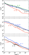 |
Fig. 3 Rotational de-excitation cross-sections of OCS by He, from the initial rotational state j = 1, 2, 3, and 4. Rotational transitions of OCS are labeled as ji → jƒ. |
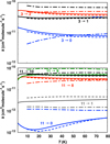 |
Fig. 4 Rotational de-excitation rate coefficients of OCS by He, from the initial rotational state j = 3, and 11 (solid lines). Rotational transitions of OCS are labeled as ji → jƒ. The rate coefficients reported by Flower (2001) are shown as dashed lines, and those scaled from Green & Chapman (1978) are also included, shown as dash-dotted lines. |
4 Summary
A new PES for the OCS+He complex was developed from a grid of ab initio energies computed at the CCSD(T) level of theory and at the completed basis set limit. The main characteristics of this surface were compared with those available in the literature, and excellent agreement was found with the surfaces presented most recently. However, our new surface is about 13% deeper than that used to calculate the only set of rate coefficients available for OCS + He, and whether or not this difference has implications for the rates needs to be explored. We employed this PES in close coupling calculations, and report a new set of rate coefficients for the lower 39 rotational states of OCS. However, the agreement with available rates is relatively good, probably because of the influence of the correct description of the long range in both surfaces, which dominates the dynamics. It is worth pointing out that this set is larger than the previously reported set for this collision.
Furthermore, we performed a comparison with the mass-scaled rate coefficients for OCS+H2. The agreement is found to be good, except for |∆j| = 2 and |∆j| ≥ 11, with both discrepancies found to be associated with the difference in the PES employed. However, as significant differences are observed for large |∆j|, and as these calculations were made from a modified surface for the OCS+He case, we recommend caution when using them in non-LTE models while new studies for this system are carried out.
Acknowledgements
Support of projects Anid/Fondo 2021 ALMA/ASTRO21-0042 and Anid/Conicyt/Fondecyt Regular/No. 1200732 is gratefully acknowledged. This research was partially supported by the supercomputing infrastructure of the NLHPC (ECM-02).
References
- Boys, S., & Bernardi, F. 1970, Mol. Phys., 19, 553 [NASA ADS] [CrossRef] [Google Scholar]
- Broquier, M., Picard-Bersellini, A., Whitaker, B., & Green, S. 1986, J. Chem. Phys., 84, 2104 [NASA ADS] [CrossRef] [Google Scholar]
- Burns, M. J., & Coy, S. L. 1984, J. Chem. Phys., 80, 3544 [NASA ADS] [CrossRef] [Google Scholar]
- Charnley, S., Ehrenfreund, P., & Kuan, Y.-J. 2001, Spectrochim. Acta A: Mol. Biomol. Spectrosc., 57, 685 [NASA ADS] [CrossRef] [Google Scholar]
- Danielson, L. J., McLeod, K. M., & Keil, M. 1987, J. Chem. Phys., 87, 239 [NASA ADS] [CrossRef] [Google Scholar]
- Drozdovskaya, M. N., van Dishoeck, E. F., Jørgensen, J. K., et al. 2018, MNRAS, 476, 4949 [Google Scholar]
- Dubernet, M., Alexander, M., Ba, Y., et al. 2013, A&A, 553, A50 [NASA ADS] [CrossRef] [EDP Sciences] [Google Scholar]
- Dunning, Thom H., J. 1989, J. Chem. Phys., 90, 1007 [NASA ADS] [CrossRef] [Google Scholar]
- Flower, D. 2001, MNRAS, 328, 147 [CrossRef] [Google Scholar]
- Gianturco, F., & Paesani, F. 2000, J. Chem. Phys., 113, 3011 [NASA ADS] [CrossRef] [Google Scholar]
- Goldsmith, P. F., & Linke, R. A. 1981, ApJ, 245, 482 [NASA ADS] [CrossRef] [Google Scholar]
- Green, S., & Chapman, S. 1978, ApJS, 37, 169 [Google Scholar]
- Herzberg, G. 1966, Electronic Spectra and Electronic Structure of Polyatomic Molecules (New York: Van Nostrand) [Google Scholar]
- Higgins, K., & Klemperer, W. 1999, J. Chem. Phys., 110, 1383 [NASA ADS] [CrossRef] [Google Scholar]
- Ho, T. S., & Rabitz, H. 1996, J. Phys. Chem., 104, 2584 [CrossRef] [Google Scholar]
- Howson, J. M., & Hutson, J. M. 2001, J. Chem. Phys., 115, 5059 [NASA ADS] [CrossRef] [Google Scholar]
- Jefferts, K., Penzias, A., Wilson, R., & Solomon, P. 1971, ApJ, 168, L111 [NASA ADS] [CrossRef] [Google Scholar]
- Li, H., & Ma, Y.-T. 2012, J. Chem. Phys., 137 [Google Scholar]
- Liu, J.-M., Zhai, Y., & Li, H. 2017, J. Chem. Phys., 147 [Google Scholar]
- Manolopoulos, D. E. 1988, PhD thesis, University of Cambridge, UK [Google Scholar]
- Matthews, H., MacLeod, J., Broten, N., Madden, S., & Friberg, P. 1987, ApJ, 315, 646 [NASA ADS] [CrossRef] [Google Scholar]
- Mauersberger, R., Henkel, C., & Chin, Y.-N. 1995, A&A, 294, 23 [NASA ADS] [Google Scholar]
- Oliaee, J. N., Brockelbank, B., McKellar, A., & Moazzen-Ahmadi, N. 2017, J. Mol. Spectrosc., 340, 36 [NASA ADS] [CrossRef] [Google Scholar]
- Paesani, F., & Whaley, K. 2004, J. Chem. Phys., 121, 4180 [NASA ADS] [CrossRef] [Google Scholar]
- Palumbo, M., Tielens, A., & Tokunaga, A. T. 1995, ApJ, 449 [Google Scholar]
- Peterson, K. A., Woon, D. E., & Dunning, T. H. 1994, J. Chem. Phys., 100, 7410 [NASA ADS] [CrossRef] [Google Scholar]
- Ross, K. A., & Willey, D. R. 2005, J. Chem. Phys., 122 [Google Scholar]
- Sadlej, J., & Edwards, W. D. 1993, Int. J. Quantum Chem., 46, 623 [CrossRef] [Google Scholar]
- Schöier, F. L., van der Tak, F. F. S., van Dishoeck, E. F., & Black, J. H. 2005, A&A, 432, 369 [Google Scholar]
- Shimanouchi, T., & Shimanouchi, T. 1980, Tables of Molecular Vibrational Frequencies (US Government Printing Office) [Google Scholar]
- Soldán, P., & Hutson, J. M. 2000, J. Chem. Phys., 112, 4415 [CrossRef] [Google Scholar]
- Stoecklin, T., Voronin, A., & Rayez, J. C. 2002, Phys. Rev. A, 66, 042703 [NASA ADS] [CrossRef] [Google Scholar]
- Stoecklin, T., Denis-Alpizar, O., Halvick, P., & Dubernet, M.-L. 2013, J. Chem. Phys., 139, 034304 [NASA ADS] [CrossRef] [Google Scholar]
- Stoecklin, T., Denis-Alpizar, O., & Halvick, P. 2015, MNRAS, 449, 3420 [NASA ADS] [CrossRef] [Google Scholar]
- Tsuge, M., & Watanabe, N. 2023, Proc. Jpn. Acad., Ser. B, 99, 103 [CrossRef] [Google Scholar]
- Urzúa-Leiva, R. & Denis-Alpizar, O. 2020, ACS Earth Space Chem., 4, 2384 [CrossRef] [Google Scholar]
- van der Tak, F. F., Boonman, A., Braakman, R., & van Dishoeck, E. F. 2003, A&A, 412, 133 [NASA ADS] [CrossRef] [EDP Sciences] [Google Scholar]
- van der Tak, F. F., Lique, F., Faure, A., Black, J. H., & van Dishoeck, E. F. 2020, Atoms, 8, 15 [NASA ADS] [CrossRef] [Google Scholar]
- Wang, Z., Feng, E., Zhang, C., & Sun, C. 2014, J. Chem. Phys., 141 [Google Scholar]
- Werner, H.-J., Knowles, P. J., Knizia, G., Manby, F. R., & Schütz, M. 2012, WIREs Comput. Mol. Sci., 2, 242 [Google Scholar]
- Wernli, M., Wiesenfeld, L., Faure, A., & Valiron, P. 2007, A&A, 464, 1147 [NASA ADS] [CrossRef] [EDP Sciences] [Google Scholar]
All Tables
Ab initio energies of the OCS+He complex at several geometrical configurations computed using different methods and basis sets.
All Figures
|
Fig. 1 Jacobi coordinates employed for studying the OCS+He complex. |
| In the text | |
|
Fig. 2 Contour plot of the PES of the OCS+He complex. Positive energies (≥50 cm−1) are shown as red contour lines in steps of 200 cm−1, and negative (≤0 cm−1) contour lines (blue) are equally spaced in steps of 5 cm−1. |
| In the text | |
|
Fig. 3 Rotational de-excitation cross-sections of OCS by He, from the initial rotational state j = 1, 2, 3, and 4. Rotational transitions of OCS are labeled as ji → jƒ. |
| In the text | |
|
Fig. 4 Rotational de-excitation rate coefficients of OCS by He, from the initial rotational state j = 3, and 11 (solid lines). Rotational transitions of OCS are labeled as ji → jƒ. The rate coefficients reported by Flower (2001) are shown as dashed lines, and those scaled from Green & Chapman (1978) are also included, shown as dash-dotted lines. |
| In the text | |
Current usage metrics show cumulative count of Article Views (full-text article views including HTML views, PDF and ePub downloads, according to the available data) and Abstracts Views on Vision4Press platform.
Data correspond to usage on the plateform after 2015. The current usage metrics is available 48-96 hours after online publication and is updated daily on week days.
Initial download of the metrics may take a while.