| Issue |
A&A
Volume 657, January 2022
|
|
|---|---|---|
| Article Number | A84 | |
| Number of page(s) | 6 | |
| Section | Galactic structure, stellar clusters and populations | |
| DOI | https://doi.org/10.1051/0004-6361/202142222 | |
| Published online | 18 January 2022 | |
APOGEE-2S view of the globular cluster Patchick 125 (Gran 3)
New metallicity and elemental abundances from high-resolution spectroscopy
1
Instituto de Astronomía, Universidad Católica del Norte, Av. Angamos 0610, Antofagasta, Chile
e-mail: This email address is being protected from spambots. You need JavaScript enabled to view it.
; This email address is being protected from spambots. You need JavaScript enabled to view it.
2
Depto. de Cs. Físicas, Facultad de Ciencias Exactas, Universidad Andrés Bello, Av. Fernández Concha 700, Las Condes, Santiago, Chile
3
Vatican Observatory, 00120 Vatican City State, Italy
4
Departamento de Astronomía, Casilla 160-C Universidad de Concepción, Concepción, Chile
Received:
14
September
2021
Accepted:
25
October
2021
Abstract
We present detailed elemental abundances, radial velocity, and orbital elements for Patchick 125, a recently discovered metal-poor globular cluster (GC) in the direction of the Galactic bulge. Near-infrared high-resolution (R ∼ 22 500) spectra of two members were obtained during the second phase of the Apache Point Observatory Galactic Evolution Experiment at Las Campanas Observatory as part of the sixteenth Data Release (DR 16) of the Sloan Digital Sky Survey. We investigated elemental abundances for four chemical species, including α- (Mg, Si), Fe-peak (Fe), and odd-Z (Al) elements. We find a metallicity covering the range from [Fe/H] = −1.69 to −1.72, suggesting that Patchick 125 likely exhibits a mean metallicity ⟨[Fe/H]⟩ ∼ −1.7, which represents a significant increase in metallicity for this cluster compared to previous low-resolution spectroscopic analyses. We also found a mean radial velocity of 95.9 km s−1, which is ∼21.6 km s−1 higher than reported in the literature. The observed stars exhibit an α-enrichment ([Mg/Fe] ≲ 0.20, and [Si/Fe] ≲ +0.30) that follows the typical trend of metal-poor GCs. The aluminum abundance ratios for the present two member stars are enhanced in [Al/Fe] ≳ +0.58, which is a typical enrichment characteristic of the so-called ‘second-generation’ of stars in GCs at similar metallicity. This supports the possible presence of the multiple-population phenomenon in Patchick 125, as well as its genuine GC nature. Further, Patchick 125 shows a low-energy, low-eccentric (< 0.4) and retrograde orbit captured by the inner Galaxy, near the edge of the bulge. We confirm that Patchick 125 is a genuine metal-poor GC, which is currently trapped in the vicinity of the Milky Way bulge.
Key words: stars: abundances / globular clusters: individual: Patchick 125 / techniques: spectroscopic
© ESO 2022
1. Introduction
Globular clusters (GCs) are among the most powerful cosmological archeology probes. Therefore, revealing in-depth details about the nature of these ancient star swarms can lead to a better understanding of the complex assembly scenarios that governed the early epochs of formation and evolution of their host galaxies. The bulge area of the Milky Way (MW) is plagued by a non-negligible fraction of GCs, many of which have remained hidden behind the high-absorption regions of the foreground field, and are affected by high levels of crowding and/or saturation by bright stars.
The combination of optical and near-infrared surveys, such as the Two-Micron All Sky Survey (2MASS; Skrutskie et al. 2006), VISTA Variables in the Vía Láctea (VVV; Minniti et al. 2010; Saito et al. 2012) and its extension (VVVX; Minniti 2018), the ESA Gaia mission (Gaia Collaboration 2016, 2018, 2021) with its unprecedented astrometric precision, and the second generation of the Apache Point Observatory Galactic Evolution Experiment survey (APOGEE-2; Majewski et al. 2017), which provides accurate spectroscopic and kinematics information, has allowed the extraordinary power of these ancient systems to be fully exploited, even in densely populated regions and those heavily obscured by the interstellar medium (ISM).
Such is the case of VVV CL001 with E(B − V)∼2.2, which was recently re-classified as the most metal-poor GC found so far –with [Fe/H] ∼ −2.45– to have survived near the bulge region (Fernández-Trincado et al. 2021a), and NGC 6330 (or Tonantzintla 1) a highly reddened, E(B − V)∼1.07 bulge GC, recently identified as the first known case of a relatively high-metallicity GC exhibiting evidence of correlation between its light- and heavy-elements and the presence of the phenomenon of multiple stellar populations (Fernández-Trincado et al. 2021b). In addition, UKS 1, a heavily reddened GC, with E(B − V)∼2.62, was recently classified as a fossil relic of the bulge based on its chemodynamics properties (Fernández-Trincado et al. 2020). These are examples of the wide gamut of highly reddened GCs examined so far towards the bulge area (see Saracino et al. 2015; Schiavon et al. 2017; Barbuy et al. 2018a,b, 2021; Fernández-Trincado et al. 2019, 2021d,c,e; Kunder & Butler 2020; Kunder et al. 2021; Geisler et al. 2021; Alonso-García et al. 2021, for other cases).
More recently, the VVV/VVVX survey has revealed that the census of Galactic GCs is still not complete, and more than 300 new low-luminosity GC candidates have been identified in the VVV/VVVX bulge+disc area toward the inner galaxy (see e.g., Minniti et al. 2020, 2021a), bulge region (Minniti et al. 2017a,b, 2018a,b; Camargo & Minniti 2019; Palma et al. 2019; Garro et al. 2021a; Obasi et al. 2021), disc region (Garro et al. 2020), the extension of the Hrid halo stream (Minniti et al. 2021b), and the Sagittarius system (Minniti et al. 2021c; Garro et al. 2021b). A few of those candidates have been confirmed as true GCs (Contreras Ramos et al. 2018; Gran et al. 2019, 2021; Barbá et al. 2019; Villanova et al. 2019; Romero-Colmenares et al. 2021; Dias et al. 2021).
In this paper we present near-infrared (NIR) elemental abundances of the heavily obscured (E(B − V)∼1.06; Garro et al. 2021c) GC Patchick 125 (originally discovered by Dana Patchick in 2016, internal communication) toward the Galactic bulge, which is positioned within 10.2″ of the centre of the GC Gran 3 (Gran et al. 2022), so both clusters are the same, and from here on we refer to this cluster as Patchick 125.
2. Spectroscopic data
We searched for high-resolution (R ∼ 22 500) H-band (1.51–1.7 μm) spectra towards the field of the GC Patchick 125 – at α = 17:05:00.70 and δ = −35:29:41.0 – in the publicly available sixteenth data release (DR16; Ahumada et al. 2020) of the APOGEE-2 survey (Majewski et al. 2017), one of the programs within the Sloan Digital Sky Survey (Blanton et al. 2017).
Stars in this field were observed using the APOGEE-2 spectrograph twin (Wilson et al. 2019) installed on the Irénée du Pont 2.5 m telescope (Bowen & Vaughan 1973) at Las Campanas Observatory (APOGEE-2S). We refer the reader to Nidever et al. (2015), Zamora et al. (2015), Holtzman et al. (2015), García Pérez et al. (2016), Zasowski et al. (2017), Smith et al. (2021), and Santana et al. (2021) for further details regarding the targeting strategy of the APOGEE-2S survey, spectra reduction, and analysis using the APOGEE Stellar Parameters and Chemical Abundance Pipeline (ASPCAP), the libraries of synthetic spectra, and the H-band line list, respectively.
The APOGEE-2S plug-plate containing the Patchick 125 field was centred on (l, b) ∼ (350°, +04°) as part of the bulge program survey containing 493 science fibres. From these stars, we identified two potential sources within 5′ of the centre of Patchick 125, which exhibit Gaia eDR3 proper motions within a 0.5 mas yr−1 radius around the mean proper motion of the cluster, μα = −3.85 ± 0.50 and μδcos(δ) = + 0.64 ± 0.39 (Garro et al., in prep.), which is in excellent agreement with the values reported in Gran et al. (2022) of namely μα = −3.78 and μδcos(δ) = + 0.66. The APOGEE-2S radial velocities of these two stars also exhibit similar kinematics, and lie in the region of the red giant branch (RGB) of Patchick 125. Figure 1 shows the main physical properties of the two newly identified members of Patchick 125 in the APOGEE-2S, Gaia eDR3, and 2MASS footprint.
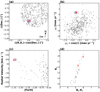 |
Fig. 1. Main physical properties of Patchick 125 stars: Panel a: spatial distribution of APOGEE-2S stars (empty circles). The position of Patchick 125 stars is shown with a navy cross, while the two cluster members analysed in this work are highlighted with red unfilled squares. A navy empty circle with a 5′ radius and centred on Patchick 125 is shown for visual aid. Panel b: the Gaia eDR3 proper motion distribution of our sample. Panel c: highlights the metallicity ([Fe/H]) versus radial velocity of APOGEE-2S stars with ASPCAP/DR16 determinations towards the Patchick 125 field (black circles) together with our BACCHUS-[Fe/H] determinations (red symbols). The blue box limited by ±0.05 dex and ±10 km s−1 and centred at [Fe/H] = −1.7 and radial velocity = 95.9 km s−1 encloses our potential cluster members. Panel d: reveals the 2MASS+Gaia eDR3 colour magnitude diagram corrected for differential reddening for Patchick stars within 3′. |
3. Atmospheric parameters
The atmospheric parameters for the two target stars were adopted in the same manner as described in Fernández-Trincado et al. (2021b), that is, we applied a simple approach of fixing Teff and log g to values determined from optical+NIR photometric bands corrected for differential reddening.
In summary, the colour-magnitude diagram (CMD) presented in Fig. 1 was corrected for differential reddening using giant stars, and adopting the reddening law of Cardelli et al. (1989) and O’Donnell (1994) and a total-to-selective absorption ratio RV = 3.1. For this purpose, we selected all RGB stars within a radius of 3 arcmin around the cluster centre that have proper motions compatible with that of Patchick 125. First, we draw a ridge line along the RGB, and for each of the selected RGB stars we calculated its distance from this line along the reddening vector. The vertical projection of this distance gives the differential optical+NIR absorption at the position of the star, while the horizontal projection gives the differential optical+NIR reddening at the position of the star. After this first step, for each star of the field we selected the three nearest RGB stars, calculated the mean reddening and absorption, and finally subtracted these mean values from its optical+NIR colours and magnitudes. We underline the fact that the number of reference stars used for the reddening correction is the result of a compromise allowing a correction that is affected as little as possible by photometric random errors whilst achieving the highest possible spatial resolution.
We obtain Teff and log from photometry by determining the differential reddening-corrected CMD of Fig. 1d. We then horizontally projected the position of each observed star until it intersected the PARSEC (Bressan et al. 2012) isochrone (chosen to have an age of 12 Gyr, a metallicity of −1.70, and an α-enhancement of 0.3.), and assumed Teff and log g to be the temperature and gravity at the point of the isochrones that has the same Ks magnitude as the star. We then applied a distance of 11.2 kpc and a reddening of E(B − V) = 1.00 to the isochrone in order to obtain the best fit to the Ks versus Bp − Ks CMD. We underline the fact that, for highly reddened objects like Patchick 125, the absorption corrections depend on their temperature. For this reason, we applied a temperature-dependent absorption correction to the isochrone. Without this, it is not possible to obtain a proper fit of the RGB, especially of the upper and cooler part.
4. Elemental abundances
The APOGEE-2S spectra of the newly identified GC Patchick 125 stars have a signal-to-noise (S/N) which is on the order of between 49 and 52 pixel−1. This S/N level makes it difficult to obtain reliable elemental abundances for some chemical species commonly accessible from the H-band of the APOGEE-2S survey. In particular, the signal from 12C14N, 12C16O, and 16OH molecules is too weak to provide reliable determinations of nitrogen, oxygen, and carbon. A visual examination of the whole spectra reveals that only four atomic elements can be accurately determined from the strengths of Mg I, Al I, Si I, and Fe I lines, as shown in Fig. 2, while the lines of other atomic elements are weak, and heavily affected by telluric features.
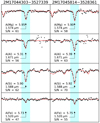 |
Fig. 2. Discovery APOGEE-2S spectra of Patchick 125 members. Examples of selected Mg I, Al I, Si I, and Fe I lines are shown. Each panel shows the best-fit synthesis (red lines) from BACCHUS compared to the observed spectra (black symbols) of selected lines (marked with black arrows, and cyan shadow bands of 3.2 × 10⁻⁴ μm wide). |
We made use of the Brussels Automatic Stellar Parameter code (BACCHUS; Masseron et al. 2016) to determine the elemental abundances of [Mg/Fe], [Al/Fe], [Si/Fe], and [Fe/H] in Patchick 125. Chemical abundances were derived from a local thermodynamics equilibrium (LTE) analysis using the BACCHUS combined with the MARCS model atmospheres (Gustafsson et al. 2008), and following the same technique as described in Fernández-Trincado et al. (2021d), and summarised here for guidance. With the atmospheric parameters determined in Sect. 3, the first step consisted in determining the metallicity from selected Fe I lines, the micro-turbulence velocity (ξt), and the convolution parameter.
With the metallicity and main atmospheric parameters fixed, we then computed the abundance of each chemical species as follows: (a) We performed a synthesis using the full set of atomic line lists (Mg I, Al I, and Si I) described in Smith et al. (2021). This set of lines is internally labelled as linelist.20170418 based on the date of creation in the format YYYYMMDD. This was used to find the local continuum level via a linear fit. (b) We then performed cosmic ray and telluric line rejections, before (c) estimating the local S/N. (d) We automatically selected a series of flux points contributing to a given absorption line, and then (e) derived abundances by comparing the observed spectrum with a set of convolved synthetic spectra characterised by different abundances. Subsequently, four different abundance determination methods were used: (1) line-profile fitting; (2) core line-intensity comparison; (3) global goodness-of-fit estimate; and (4) an equivalent-width comparison. Each diagnostic yields validation flags. Based on these flags, a decision tree then rejects or accepts each estimate, keeping the best-fit abundance. We adopted the ξ2 diagnostic as the abundance because of its robustness. However, we stored the information from the other diagnostics, including the standard deviation between all four methods.
Table 1 lists the final atmospheric parameters and the measured elemental abundances, while Fig. 2 shows the line-by-line spectrum synthesis with the BACCHUS code around selected atomic Mg I, Al I, Si I, and Fe I lines. The uncertainties reported in Table 1 were determined in the same manner as described in Fernández-Trincado et al. (2019) by varying the atmospheric parameters one at a time by ±100 K for the effective temperature, ±0.30 cgs for the surface gravity, and ±0.05 km s−1 for the microturbulent velocity, which are typical but conservative values. Thus, the reported uncertainties are defined as  .
.
APOGEE-2S elemental abundances of Patchick 125.
5. Abundance analysis
We find that stars in Patchick 125 are as metal poor as −1.69 and −1.72, suggesting a mean metallicity of ⟨[Fe/H]⟩ ∼ −1.70, which is consistent with recent photometric estimates for this cluster, [Fe/H] = −1.8 ± 0.2 (Garro et al., in prep.). With a sample size of two stars, we cannot comment on the existence of a metallicity spread in Patchick 125. However, we plan to investigate the cluster’s metallicity distribution in a future spectroscopic follow-up study.
It is important to note that Gran et al. (2022) determined a mean metallicity of ⟨[Fe/H]⟩ = −2.33 for Patchick 125 (or Gran 3), which is ∼0.63 more metal poor than our determinations. However, their methodology, which relies on the relation between CaT EW and the magnitude of the HB in the Johnson V filter, tends to be less precise than our high-resolution determinations which rely directly on the Fe I lines, as this cluster lies in a very highly reddened region, with E(B − V) > 1, and extinction Av ∼ 2.37 (Gran et al. 2022).
The odd-Z element Al was found to be enhanced in the two Patchick 125 stars, placing this cluster well above the typical [Al/Fe] levels seen in other GCs, as can be seen in the middle panel in Fig. 3. The high [Al/Fe] abundance ratios measured in Patchick 125 could belong to the so-called second-generation population, which could explain the apparent overabundance in Al compared to other GCs. Therefore, with the current limited sample in Patchick 125, it is not possible to reach a firm conclusion about the origin of this cluster based on the observed [Al/Fe].
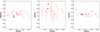 |
Fig. 3. BACCHUS distribution of [Fe/H] vs. [Mg/Fe] (left), [Al/Fe] (middle), and [Si/Fe] (right) for GCs (red open symbols) analysed in Mészáros et al. (2020). Patchick 125 members are highlighted with black star symbols. |
The α-element Mg is slightly overabundant compared to the Sun. Figure 3 shows that these two stars exhibit slightly lower [Mg/Fe] abundance ratios compared to those of metal-poor GCs, which could be due to the fact that these stars belong to the ‘second-generation’ population with a high-aluminum enrichment, and therefore do not reflect the mean [Mg/Fe] enrichment of the cluster. Unfortunately, in this case, the [Mg/Fe] abundances alone are not useful indicators with which to distinguish between an in situ and accreted origin for this cluster.
The second measured α-element Si shows that Patchick 125 stars exhibit [Si/Fe] abundance ratios comparable to those of metal-poor GCs, as shown in the right panel of Fig. 3. It is important to note that the high [Al/Fe] enrichment well above +0.58 observed in Patchick 125 stars is typical among the so-called second-generation stars in GCs at similar metallicity (M 55; Mészáros et al. 2020, for instance), and is unlikely to be seen in dwarf galaxy populations (Shetrone et al. 2001; Hasselquist et al. 2017, 2021), thus supporting the genuine GC nature of Patchick 125.
6. Dynamical properties of Patchick 125
We made use of the GravPot16 model1 to predict the ensemble of orbits associated with Patchick 125.
6.1. Model
We adopted the same GravPot16 model configuration as described in Romero-Colmenares et al. (2021), which consists of a boxy/peanut bar structure in the bulge region along with other composite stellar components belonging to the thin and thick discs, ISM, an oblate Hernquist stellar halo, and a dark-matter component characterised by an isothermal sphere truncated at Rgal ∼ 100 kpc. For a more detailed description of the functional forms of the gravitational potential of each component, we refer the readers to a forthcoming paper (GravPot16; Fernández-Trincado et al., in prep.).
The structural parameters of our bar model (mass, present-day orientation, and pattern speed) are 1.1 × 10¹⁰ M⊙, 20°, and Ωbar = 41 km s−1 kpc (Sanders et al. 2019), respectively, consistent with observational estimates. The bar scale lengths are x0 = 1.46 kpc, y0 = 0.49 kpc, and z0 = 0.39 kpc, where the effective boundary (or cut-off radius) of the bar on the x-axis has a semi-major axis of 3.43 kpc.
For reference, the Galactic convention adopted in this work is: x-axis oriented towards l = 0° and b = 0°, y-axis oriented towards l = 90° and b = 0°, and the disc rotates towards l = 90°; the velocity is also oriented along these directions. Following this convention, the Sun’s orbital velocity vectors are [U⊙,V⊙,W⊙] = 11.1, 12.24, 7.25] km s−1 (Brunthaler et al. 2011). The model has been rescaled to the Sun’s Galactocentric distance of 8.3 kpc, and the local rotation velocity of 244.5 km s−1 (Sofue 2015).
6.2. Orbit
To compute the orbits of Patchick 125 we adopted the following three initial conditions: (i) The mean proper motions for Patchick 125 were adopted from the values determined by Garro et al. (2021c), that is, μα = −3.85 ± 0.50 and μδcos(δ) = + 0.64 ± 0.39; (ii) Garro et al. (2021c) measured distances of D = 11.2 kpc and 10.9 kpc to this GC based on the optical and NIR CMDs, respectively. They also identified two RR Lyrae variable stars as cluster members based on their matching positions, magnitudes, and Gaia proper motions. These are RR Lyrae-type ab stars Gaia DR2 5977224553266268928 and 5977223144516980608 from Clementini et al. (2019), both located at about 80″ from the cluster centre. We are able to check the determination of the distance for this cluster using the NIR photometry of these RRab stars; their magnitudes are Ks = 14.845 ± 0.025 and 14.775 ± 0.024 mag, their colours are J − Ks = 0.785 ± 0.03 and 0.589 ± 0.03 mag, and their periods are P = 0.601940 and P = 0.738296 days, respectively. Using the latest NIR PLZ relations of Bhardwaj et al. (2021) for [Fe/H] = −1.7, and adopting a field extinction of AK = 0.327 mag from Schlafly & Finkbeiner (2011), their distances are D = 10.66 ± 0.30 kpc and 11.42 ± 0.30 kpc, respectively. This yields a mean cluster distance of D = 11.0 ± 0.5 kpc, which is in agreement with the values obtained by Garro et al. (2021a,b,c), and our (see Sect. 3). (iii) The cluster mean radial velocity was assumed to be 95.9 km s−1, which was obtained from our APOGEE-2S data. This adopted radial velocity value is in reasonable agreement with the value reported by (Gran et al. 2022), of namely 74.23 ± 2.70 km s−1, which is lower than our value by ∼21.6 km s−1. This difference in radial velocity could be due to systematic errors between the low resolution of the MUSE spectra and the high resolution of the APOGEE-2S spectra. However, we note that by adopting both values in radial velocity, our conclusions regarding the dynamical behaviour of Patchick 125 are not strongly affected. For our orbit computations, we assumed an error for the cluster radial velocity of the order of 10 km s−1.
We computed an ensemble of orbits by adopting a simple Monte Carlo approach and the Runge-Kutta algorithm of seventh to eighth order elaborated by Fehlberg (1968). The uncertainties in the input data were randomly propagated as 1σ variation in a Gaussian Monte Carlo resampling. Thus, we ran 10 000 orbits, computed backwards in time for 1.5 Gyr. The 50th percentile of the orbital elements were found for these 10 000 realisations, with uncertainty ranges given by the 16th and 84th percentiles.
The resulting orbital elements are listed in Table 2 for three different values of Ωbar, which was varied in steps of 10 km s−1 kpc in order to check for any significant impact of variations of this parameter. The minimal and maximum values of the z-component of the angular momentum in the inertial frame are also listed in this table, because this quantity is not conserved in a model with non-axisymmetric structures like GravPot16. Table 2 and Fig. 4 also show that our orbit results are not strongly affected by variations in Ωbar.
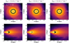 |
Fig. 4. Ensemble of 10 000 orbits of Patchick 125 by considering the errors on the observables, projected on the equatorial and meridional Galactic planes in the inertial reference frame, with a bar pattern speed of 31, 41, and 51 km s−1 and integrated over the past 1.5 Gyr. The red and orange colours correspond to more probable regions of the space, which are crossed most frequently by the simulated orbits. The black line shows the orbit of Patchick 125 from the observables without error bars. The white dashed line indicates the Sun’s radius. The white filled and unfilled star symbols indicate the initial and final positions of the cluster, respectively. |
Orbital elements for Patchick 125.
Figure 4 shows the probability densities of the resulting ensemble of orbits projected on the equatorial and meridional Galactic planes in the inertial reference frame. The red and yellow colours correspond to more probable regions of space, which are crossed more frequently by the simulated orbits.
Patchick 125 is found to have a low eccentricity and retrograde orbital configuration (see Table 2), which has perigalactocentric distances with incursions inside the cut-off radius of the bar, apogalactocentric distances (rapo ∼ 3.98–4.51 kpc) at the edge of the MW bulge (redge ∼ 3 kpc; Barbuy et al. 2018a; Pérez-Villegas et al. 2020), and vertical excursions from the Galactic plane, |Z|max ≲ 3.2 kpc, which are similar to those recently found by Gran et al. (2022). Our observations caught Patchick 125 near the apocentre of its orbit.
7. Conclusions
We present the first high-resolution NIR spectral examination of two newly identified members of the GC Patchick 125, for which we measure precise radial velocities using data from the APOGEE-2S survey. Patchick 125 is located in a region of high interstellar reddening in the direction of the MW bulge. We employed the BACCHUS code to manually determine reliable abundance ratios for [Mg/Fe], [Al/Fe], [Si/Fe], and [Fe/H] from the strength of Mg I, Al I, Si I, and Fe I lines, the intensities of which are clearly distinguished from the local continuum level (see Fig. 2).
Overall, Patchick 125 hosts metal-poor stars with a [Fe/H] abundance ratio of between −1.72 and −1.69, which is consistent with previous photometric estimates for this cluster. The α enrichment, [Mg/Fe] ≲ +0.20, and in particular [Si/Fe] ≲ +0.30, places Patchick 125 among typical metal-poor GCs. We identified a high enrichment in aluminum ([Al/Fe] > +0.58) among the Patchick 125 members, which are therefore likely associated with the so-called second-generation population. Such a value is typical among metal-poor GCs, thus reinforcing the GC nature of Patchick 125. With only two stars, it is not possible to make any meaningful conclusions about the radial velocity dispersion or metallicity spread of this cluster.
We find that Patchick 125 is a typical metal-poor GC, which lies on a low-eccentricity and retrograde orbit and currently resides inside the corotation radius (< 5.7 kpc), trapped in a low-energy orbit at the edge of the Galactic bulge.
Acknowledgments
The author is grateful for the enlightening feedback from the anonymous referee. J.G.F-T acknowledges partial support from Comité Mixto ESO-Chile 2021. D.M. gratefully acknowledges support from the Chilean Centro de Excelencia en Astrofísica y Tecnologías Afines (CATA) BASAL grant AFB-170002. ERG acknowledges support from ANID PhD scholarship No. 21210330 The SDSS-IV/APOGEE-2S survey made this study possible. This work has made use of data from the European Space Agency (ESA) mission Gaia (http://www.cosmos.esa.int/gaia), processed by the Gaia Data Processing and Analysis Consortium (DPAC, http://www.cosmos.esa.int/web/gaia/dpac/consortium). Funding for the DPAC has been provided by national institutions, in particular the institutions participating in the Gaia Multilateral Agreement. J.G.F-T gratefully acknowledges the grant support provided by Proyecto Fondecyt Iniciación No. 11220340, and also from ANID Concurso de Fomento a la Vinculación Internacional para Instituciones de Investigación Regionales (Modalidad corta duración) Proyecto No. FOVI210020, and from the Joint Committee ESO-Government of Chile 2021 (ORP 023/2021).
References
- Ahumada, R., Prieto, C. A., Almeida, A., et al. 2020, ApJS, 249, 3 [Google Scholar]
- Alonso-García, J., Smith, L. C., Catelan, M., et al. 2021, A&A, 651, A47 [NASA ADS] [CrossRef] [EDP Sciences] [Google Scholar]
- Barbá, R. H., Minniti, D., Geisler, D., et al. 2019, ApJ, 870, L24 [CrossRef] [Google Scholar]
- Barbuy, B., Chiappini, C., & Gerhard, O. 2018a, ARA&A, 56, 223 [Google Scholar]
- Barbuy, B., Muniz, L., Ortolani, S., et al. 2018b, A&A, 619, A178 [NASA ADS] [CrossRef] [EDP Sciences] [Google Scholar]
- Barbuy, B., Cantelli, E., Muniz, L., et al. 2021, A&A, 654, A29 [NASA ADS] [CrossRef] [EDP Sciences] [Google Scholar]
- Bhardwaj, A., Rejkuba, M., Sloan, G. C., Marconi, M., & Yang, S. C. 2021, ApJ, 922, 20 [CrossRef] [Google Scholar]
- Blanton, M. R., Bershady, M. A., Abolfathi, B., et al. 2017, AJ, 154, 28 [Google Scholar]
- Bowen, I. S., & Vaughan, A. H. J. 1973, Appl. Opt., 12, 1430 [Google Scholar]
- Bressan, A., Marigo, P., Girardi, L., et al. 2012, MNRAS, 427, 127 [NASA ADS] [CrossRef] [Google Scholar]
- Brunthaler, A., Reid, M. J., Menten, K. M., et al. 2011, Astron. Nachr., 332, 461 [Google Scholar]
- Camargo, D., & Minniti, D. 2019, MNRAS, 484, L90 [Google Scholar]
- Cardelli, J. A., Clayton, G. C., & Mathis, J. S. 1989, ApJ, 345, 245 [Google Scholar]
- Clementini, G., Ripepi, V., Molinaro, R., et al. 2019, A&A, 622, A60 [NASA ADS] [CrossRef] [EDP Sciences] [Google Scholar]
- Contreras Ramos, R., Minniti, D., Fernández-Trincado, J. G., et al. 2018, ApJ, 863, 78 [Google Scholar]
- Dias, B., Palma, T., Minniti, D., et al. 2021, A&A, 657, A67 [Google Scholar]
- Fehlberg, E. 1968, NASA TR R-287 [Google Scholar]
- Fernández-Trincado, J. G., Zamora, O., Souto, D., et al. 2019, A&A, 627, A178 [Google Scholar]
- Fernández-Trincado, J. G., Minniti, D., Beers, T. C., et al. 2020, A&A, 643, A145 [Google Scholar]
- Fernández-Trincado, J. G., Minniti, D., Souza, S. O., et al. 2021a, ApJ, 908, L42 [Google Scholar]
- Fernández-Trincado, J. G., Beers, T. C., Barbuy, B., et al. 2021b, ApJ, 918, L9 [CrossRef] [Google Scholar]
- Fernández-Trincado, J. G., Beers, T. C., Minniti, D., et al. 2021c, A&A, 647, A64 [EDP Sciences] [Google Scholar]
- Fernández-Trincado, J. G., Beers, T. C., Minniti, D., et al. 2021d, A&A, 648, A70 [Google Scholar]
- Fernández-Trincado, J. G., Villanova, S., Geisler, D., et al. 2021e, A&A, accepted [arXiv:2110.10700] [Google Scholar]
- Gaia Collaboration (Brown, A. G. A., et al.) 2016, A&A, 595, A2 [NASA ADS] [CrossRef] [EDP Sciences] [Google Scholar]
- Gaia Collaboration (Brown, A. G. A., et al.) 2018, A&A, 616, A1 [NASA ADS] [CrossRef] [EDP Sciences] [Google Scholar]
- Gaia Collaboration (Brown, A. G. A., et al.) 2021, A&A, 650, C3 [EDP Sciences] [Google Scholar]
- García Pérez, A. E., Allende Prieto, C., Holtzman, J. A., et al. 2016, AJ, 151, 144 [Google Scholar]
- Garro, E. R., Minniti, D., Gómez, M., et al. 2020, A&A, 642, L19 [EDP Sciences] [Google Scholar]
- Garro, E. R., Minniti, D., Gómez, M., et al. 2021a, A&A, 649, A86 [NASA ADS] [CrossRef] [EDP Sciences] [Google Scholar]
- Garro, E. R., Minniti, D., Gómez, M., & Alonso-García, J. 2021b, A&A, 654, A23 [NASA ADS] [CrossRef] [EDP Sciences] [Google Scholar]
- Garro, E. R., Minniti, D., Gómez, M., et al. 2021c, A&A, accepted [arXiv:2112.13591] [Google Scholar]
- Geisler, D., Villanova, S., O’Connell, J. E., et al. 2021, A&A, 652, A157 [NASA ADS] [CrossRef] [EDP Sciences] [Google Scholar]
- Gran, F., Zoccali, M., Contreras Ramos, R., et al. 2019, A&A, 628, A45 [NASA ADS] [CrossRef] [EDP Sciences] [Google Scholar]
- Gran, F., Zoccali, M., Rojas-Arriagada, A., et al. 2021, MNRAS, 504, 3494 [NASA ADS] [CrossRef] [Google Scholar]
- Gran, F., Zoccali, M., Saviane, I., et al. 2022, MNRAS, 509, 4962 [Google Scholar]
- Gustafsson, B., Edvardsson, B., Eriksson, K., et al. 2008, A&A, 486, 951 [NASA ADS] [CrossRef] [EDP Sciences] [Google Scholar]
- Hasselquist, S., Shetrone, M., Smith, V., et al. 2017, ApJ, 845, 162 [Google Scholar]
- Hasselquist, S., Hayes, C. R., Lian, J., et al. 2021, ApJ, 923, 172 [NASA ADS] [CrossRef] [Google Scholar]
- Holtzman, J. A., Shetrone, M., Johnson, J. A., et al. 2015, AJ, 150, 148 [Google Scholar]
- Kunder, A. M., & Butler, E. 2020, AJ, 160, 241 [NASA ADS] [CrossRef] [Google Scholar]
- Kunder, A., Crabb, R. E., Debattista, V. P., Koch-Hansen, A. J., & Huhmann, B. M. 2021, AJ, 162, 86 [NASA ADS] [CrossRef] [Google Scholar]
- Majewski, S. R., Schiavon, R. P., Frinchaboy, P. M., et al. 2017, AJ, 154, 94 [NASA ADS] [CrossRef] [Google Scholar]
- Masseron, T., Merle, T., & Hawkins, K. 2016, BACCHUS: Brussels Automatic Code for Characterizing High Accuracy Spectra Astrophysics Source Code Library, [record ascl:1605.004] [Google Scholar]
- Mészáros, S., Masseron, T., García-Hernández, D. A., et al. 2020, MNRAS, 492, 1641 [Google Scholar]
- Minniti, D. 2018, in The Vatican Observatory, Castel Gandolfo: 80th Anniversary Celebration, eds. G. Gionti, & J. B. Kikwaya Eluo, 51, 63 [Google Scholar]
- Minniti, D., Lucas, P. W., Emerson, J. P., et al. 2010, New Astron., 15, 433 [Google Scholar]
- Minniti, D., Geisler, D., Alonso-García, J., et al. 2017a, ApJ, 849, L24 [CrossRef] [Google Scholar]
- Minniti, D., Palma, T., Dékány, I., et al. 2017b, ApJ, 838, L14 [Google Scholar]
- Minniti, D., Schlafly, E. F., Palma, T., et al. 2018a, ApJ, 866, 12 [Google Scholar]
- Minniti, D., Fernández-Trincado, J. G., Ripepi, V., et al. 2018b, ApJ, 869, L10 [Google Scholar]
- Minniti, D., Gómez, M., Pullen, J. B., et al. 2020, Res. Notes Am. Astron. Soc., 4, 218 [Google Scholar]
- Minniti, D., Fernández-Trincado, J. G., Smith, L. C., et al. 2021a, A&A, 648, A86 [NASA ADS] [CrossRef] [EDP Sciences] [Google Scholar]
- Minniti, D., Fernández-Trincado, J. G., Gómez, M., et al. 2021b, A&A, 650, L11 [NASA ADS] [CrossRef] [EDP Sciences] [Google Scholar]
- Minniti, D., Ripepi, V., Fernández-Trincado, J. G., et al. 2021c, A&A, 647, L4 [NASA ADS] [CrossRef] [EDP Sciences] [Google Scholar]
- Nidever, D. L., Holtzman, J. A., Allende Prieto, C., et al. 2015, AJ, 150, 173 [NASA ADS] [CrossRef] [Google Scholar]
- Obasi, C., Gómez, M., Minniti, D., & Alonso-García, J. 2021, A&A, 654, A39 [NASA ADS] [CrossRef] [EDP Sciences] [Google Scholar]
- O’Donnell, J. E. 1994, ApJ, 422, 158 [Google Scholar]
- Palma, T., Minniti, D., Alonso-García, J., et al. 2019, MNRAS, 487, 3140 [Google Scholar]
- Pérez-Villegas, A., Barbuy, B., Kerber, L. O., et al. 2020, MNRAS, 491, 3251 [Google Scholar]
- Romero-Colmenares, M., Fernández-Trincado, J. G., Geisler, D., et al. 2021, A&A, 652, A158 [NASA ADS] [CrossRef] [EDP Sciences] [Google Scholar]
- Saito, R. K., Hempel, M., Minniti, D., et al. 2012, A&A, 537, A107 [NASA ADS] [CrossRef] [EDP Sciences] [Google Scholar]
- Sanders, J. L., Smith, L., & Evans, N. W. 2019, MNRAS, 488, 4552 [NASA ADS] [CrossRef] [Google Scholar]
- Santana, F. A., Beaton, R. L., Covey, K. R., et al. 2021, AJ, 162, 303 [NASA ADS] [CrossRef] [Google Scholar]
- Saracino, S., Dalessandro, E., Ferraro, F. R., et al. 2015, ApJ, 806, 152 [NASA ADS] [CrossRef] [Google Scholar]
- Schiavon, R. P., Johnson, J. A., Frinchaboy, P. M., et al. 2017, MNRAS, 466, 1010 [NASA ADS] [CrossRef] [Google Scholar]
- Schlafly, E. F., & Finkbeiner, D. P. 2011, ApJ, 737, 103 [Google Scholar]
- Shetrone, M. D., Côté, P., & Sargent, W. L. W. 2001, ApJ, 548, 592 [NASA ADS] [CrossRef] [Google Scholar]
- Skrutskie, M. F., Cutri, R. M., Stiening, R., et al. 2006, AJ, 131, 1163 [NASA ADS] [CrossRef] [Google Scholar]
- Smith, V. V., Bizyaev, D., Cunha, K., et al. 2021, AJ, 161, 254 [NASA ADS] [CrossRef] [Google Scholar]
- Sofue, Y. 2015, PASJ, 67, 75 [Google Scholar]
- Villanova, S., Monaco, L., Geisler, D., et al. 2019, ApJ, 882, 174 [NASA ADS] [CrossRef] [Google Scholar]
- Wilson, J. C., Hearty, F. R., Skrutskie, M. F., et al. 2019, PASP, 131 [Google Scholar]
- Zamora, O., García-Hernández, D. A., Allende Prieto, C., et al. 2015, AJ, 149, 181 [CrossRef] [Google Scholar]
- Zasowski, G., Cohen, R. E., Chojnowski, S. D., et al. 2017, AJ, 154, 198 [Google Scholar]
All Tables
All Figures
|
Fig. 1. Main physical properties of Patchick 125 stars: Panel a: spatial distribution of APOGEE-2S stars (empty circles). The position of Patchick 125 stars is shown with a navy cross, while the two cluster members analysed in this work are highlighted with red unfilled squares. A navy empty circle with a 5′ radius and centred on Patchick 125 is shown for visual aid. Panel b: the Gaia eDR3 proper motion distribution of our sample. Panel c: highlights the metallicity ([Fe/H]) versus radial velocity of APOGEE-2S stars with ASPCAP/DR16 determinations towards the Patchick 125 field (black circles) together with our BACCHUS-[Fe/H] determinations (red symbols). The blue box limited by ±0.05 dex and ±10 km s−1 and centred at [Fe/H] = −1.7 and radial velocity = 95.9 km s−1 encloses our potential cluster members. Panel d: reveals the 2MASS+Gaia eDR3 colour magnitude diagram corrected for differential reddening for Patchick stars within 3′. |
| In the text | |
|
Fig. 2. Discovery APOGEE-2S spectra of Patchick 125 members. Examples of selected Mg I, Al I, Si I, and Fe I lines are shown. Each panel shows the best-fit synthesis (red lines) from BACCHUS compared to the observed spectra (black symbols) of selected lines (marked with black arrows, and cyan shadow bands of 3.2 × 10⁻⁴ μm wide). |
| In the text | |
|
Fig. 3. BACCHUS distribution of [Fe/H] vs. [Mg/Fe] (left), [Al/Fe] (middle), and [Si/Fe] (right) for GCs (red open symbols) analysed in Mészáros et al. (2020). Patchick 125 members are highlighted with black star symbols. |
| In the text | |
|
Fig. 4. Ensemble of 10 000 orbits of Patchick 125 by considering the errors on the observables, projected on the equatorial and meridional Galactic planes in the inertial reference frame, with a bar pattern speed of 31, 41, and 51 km s−1 and integrated over the past 1.5 Gyr. The red and orange colours correspond to more probable regions of the space, which are crossed most frequently by the simulated orbits. The black line shows the orbit of Patchick 125 from the observables without error bars. The white dashed line indicates the Sun’s radius. The white filled and unfilled star symbols indicate the initial and final positions of the cluster, respectively. |
| In the text | |
Current usage metrics show cumulative count of Article Views (full-text article views including HTML views, PDF and ePub downloads, according to the available data) and Abstracts Views on Vision4Press platform.
Data correspond to usage on the plateform after 2015. The current usage metrics is available 48-96 hours after online publication and is updated daily on week days.
Initial download of the metrics may take a while.