| Issue |
A&A
Volume 657, January 2022
|
|
|---|---|---|
| Article Number | A118 | |
| Number of page(s) | 10 | |
| Section | The Sun and the Heliosphere | |
| DOI | https://doi.org/10.1051/0004-6361/202141401 | |
| Published online | 20 January 2022 | |
Statistical properties of Hα jets in the polar coronal hole and their implications in coronal activities⋆
1
Shandong Provincial Key Laboratory of Optical Astronomy and Solar-Terrestrial Environment, Institute of Space Sciences, Shandong University, Weihai, 264209 Shandong, PR China
e-mail: This email address is being protected from spambots. You need JavaScript enabled to view it.
2
Now at School of Earth and Space Sciences, Peking University, Beijing 100871, PR China
Received:
27
May
2021
Accepted:
22
October
2021
Abstract
Context. Dynamic features such as chromospheric jets, transition region network jets, coronal plumes, and coronal jets are abundant in the network regions of polar coronal holes on the Sun.
Aims. We investigate the relationship between chromospheric jets and coronal activities, such as coronal plumes and jets.
Methods. We analyzed observations of a polar coronal hole including the filtergrams taken by the New Vacuum Solar Telescope at the Hα − 0.6 Å to study the Hα jets, as well as the Atmospheric Imaging Assembly 171 Å images to follow the evolution of coronal activities.
Results. The Hα jets are persistent in the network regions, with only some regions (denoted as R1–R5) rooted in discernible coronal plumes. With an automated method, we identified and tracked 1320 Hα jets in the network regions. We find that the average lifetime, height, and ascending speed of the Hα jets are 75.38 s, 2.67 Mm, 65.60 km s−1, respectively. The Hα jets rooted in R1–R5 are higher and faster than those in the others. We also find that propagating disturbances (PDs) in coronal plumes have a close connection with the Hα jets. The speeds of 28 out of 29 Hα jets associated with PDs are ≳50 km s−1. In the case of a coronal jet, we find that the speeds in both the coronal jet and the Hα jet are over 150 km s−1, suggesting that both cool and hot jets can be coupled.
Conclusions. Based on our analyses, it is evident that more dynamic Hα jets could release their energy to the corona, which might be the result of a Kelvin-Helmholtz instability developing or that of small-scale magnetic activities. We suggest that chromospheric jets, transition region network jets, and ray-like features in the corona are coherent phenomena that serve as important vehicles for cycling energy and mass in the solar atmosphere.
Key words: Sun: chromosphere / Sun: corona
Movies associated to Figs. 1, 5, and 7 are available at https://www.aanda.org
© ESO 2022
1. Introduction
The chromosphere is a dynamic and highly structured region linking the photosphere and the corona. In the photosphere, magnetic flux tubes make up the magnetic network, which expands upward and appears as bright patches in the chromosphere – namely, the chromospheric network. Therefore, the network boundaries in the chromosphere spatially coincide with the magnetic network concentrations in the photosphere. The chromospheric network boundaries are abundant in fine-scale, jet-like features, which are referred to as spicules at the limb, mottles in the quiet sun, and fibrils in active regions (e.g., Beckers 1968; Rouppe van der Voort et al. 2007; De Pontieu et al. 2007a, etc.). Spicules have been studied for more than a century and are still one of the most popular topics in the present day (see e.g., Beckers 1968; Sterling 2000; Tsiropoula et al. 2012, for extensive overviews).
Based on high spatio-temporal resolution observations, De Pontieu et al. (2007b) pointed out the existence of two different types of spicules (Type I and Type II). A typical characteristic of Type I spicules (also known as traditional spicules) is that they move up and down with ascending speeds in the range of 15 − 40 km s−1. Type I spicules have lifetimes of 150 − 400 s and heights of 4 − 8 Mm, and they are believed to result from magnetoacoustic shocks. In contrast, Type II spicules rise with much higher speeds of ∼100 km s−1 and disappear rapidly with shorter lifetimes of 50 − 150 s. It has been suggested that Type II spicules are driven by magnetic reconnections. De Pontieu et al. (2007c) found that the Type II spicules also undergo sideways swaying motion, which is signature of Alfvén waves permeating with enough energy to heat the corona and accelerate the solar wind. With high-quality observations, the Type II spicules have been found to combine three different types of motions: field-aligned flows, swaying motions, and torsional motions, of which swaying and torsional motions are considered signs of spicules propagating along their axis with Alfvén waves at high speeds ranging from 100−300 km s−1. With multi-wavelength observations, Type II spicules often appeared to heat to the transition region temperatures, even up to the coronal temperatures (e.g., De Pontieu et al. 2011, 2014; Rouppe van der Voort et al. 2015). Based on advanced 2.5D radiative MHD simulations, Martínez-Sykora et al. (2017) reproduced many observed properties of type II spicules with ∼100 km s−1 speeds and ∼10 Mm heights, and also revealed that spicules could heat plasma to the corona via the dissipation of current which is due to ambipolar diffusion. This subsequent numerical study showed that the dissipation through ambipolar diffusion of electrical currents could also explain why the observed spicules could reach a speed exceeding 100 km s−1 and get heated to coronal temperatures (De Pontieu et al. 2017).
In active region plage regions, Hansteen et al. (2006) and De Pontieu et al. (2007a) analyzed Hα observations and found that fibrils appear as short, dynamic, and spicule-like features with lifetimes of between 3 and 6 min and exhibiting quasi-periodicity. These dynamic fibrils undergo their ascent and descent motions with velocities of 10 − 35 km s−1 at the initial phase, which are similar to that of Type I spicules. Moreover, the numerical simulations demonstrated that these fibril-like features also show wave-behaviors. That could be formed when flows and oscillations leak from magnetic flux concentrations into the chromosphere (e.g., Hansteen et al. 2006; De Pontieu et al. 2007a; Heggland et al. 2007, 2011).
In quiet-Sun regions, mottles are shown as dark and spicule-like features against the disk in the wings of Hα. Similar to fibrils, the motions of some mottles also follow a parabolic path and they can be driven by shock waves (e.g., Rouppe van der Voort et al. 2007; De Pontieu et al. 2007d).
With the spectroscopic data, Langangen et al. (2008) firstly used Ca II 854.2 nm line to investigate the rapid blueshifted excursions (RBEs) on a disk, which are observed as a sudden widening of line profile in the blue wing without an associated redshift. Combined with SJ images of Hα, these RBEs are shown to be narrow streaks emanating from the network (Rouppe van der Voort et al. 2009). The RBEs show velocities of 15 − 20 km s−1 and a mean lifetime of 45 s. There are ∼105 RBEs on the surface of disk at any moment. Recently, Sekse et al. (2012, 2013) found that RBEs also undergo three kinds of motions (as in the case of spicules). Owing to the similarity, RBEs are interpreted as the on-disk counterparts of Type II spicules and suggested to result from magnetic reconnection (Rouppe van der Voort et al. 2009).
Jet-like features are not only seen in the chromosphere, but also in the transition region and corona. In the transition region, network jets are small-scale structures, having lifetimes of 20 − 80 s and speeds of 80 − 250 km s−1. A number of them appear as “inverse-Y” shape, which is expected to be driven by magnetic reconnection (Tian et al. 2014). In the corona, coronal jets appear as transient collimated beams. More findings suggest that coronal jets are driven by magnetic reconnection and may be the source of mass and energy input to the upper solar atmosphere and the solar wind (see Raouafi et al. 2016, and the references therein). Plumes belong to another type of collimated structures, which are relatively large and stable (see Wilhelm et al. 2011, and the references therein) and might supply plasma and energy for solar wind (e.g., Tian et al. 2010, 2011; Fu et al. 2014; Liu et al. 2015; Huang et al. 2021).
There are PDs in coronal plumes with 10%−20% intensity variations, periods of 10−30 min and speeds of 75−170 km s−1 (e.g., DeForest & Gurman 1998; Krishna Prasad et al. 2011). Furthermore, Tian et al. (2011) discovered that high-speed quasi-periodic outflows could be found in both plumes and inter-plume regions, and their speeds are similar to that of PDs. These outflows were suggested to be responsible for the generation of PDs (McIntosh et al. 2010). By following the evolution of spicules, Jiao et al. (2015) and Pant et al. (2015) concluded that the spicules can trigger PDs.
In the base of coronal plumes, Raouafi et al. (2008) found that coronal jets could contribute to rise and change in terms of brightness in the pre-existing plumes. Given that those coronal jets are rooted in the chromospheric network and are mainly triggered by magnetic reconnection, coronal plumes could also be powered by magnetic reconnection (for an extensive overview, see Raouafi et al. 2016). Furthermore, Raouafi & Stenborg (2014) and Panesar et al. (2018) found that a great number of jets and transient bright points frequently occurred in the bases of coronal plumes and these features could be the main energy source for coronal plumes. In fact, the scenario that coronal plumes are driven by the magnetic reconnection between the unipolarity magnetic features and nearby small-scale bipolar was proposed much earlier (e.g., Wang & Sheeley 1995; Wang et al. 1997; Wang & Muglach 2008).
Since there are many kinds of jet-like features rooted in network regions, it is natural to ask whether there is any connection among them. With the aim of approaching this question Qi et al. (2019, hereafter Paper I) developed an automatic method to identify and track network jets. They statistically analyzed a set of transition region network jets in the same network region, and they found that network jets in the root of coronal plumes have lifetime, height, and speed averaging at 45.6 s, 8.1″ and 131 km s−1, significantly more dynamic than those in regions without any discernible plumes, which have longer lifetimes at 50.2 s, smaller heights at 5.5″, and lower speeds at 89 km s−1, on average. Paper I suggests that only more energetic network jets (likely with speeds more than 100 km s−1) can feed plasma to the corona. In the present study, we further investigate the possible relationship between chromospheric jet-like features (e.g., spicules, fibrils, mottles, or RBEs) and coronal activities. To achieve this, we analyzed data obtained with the ground-based 1-m New Vacuum Solar Telescope (NVST) (Liu et al. 2014; Xiang et al. 2016) installed at the Fuxian Lake Solar Observing Stations and operated by Yunnan Astronomical Observatories in China, as well as the space-borne Atmospheric Imaging Assembly (AIA) (Lemen et al. 2012) and the Helioseismic and Magnetic Imager (HMI, Schou et al. 2012) aboard the Solar Dynamics Observatory (SDO, Pesnell et al. 2012).
The paper is organized as follows. The observations and methodology are described in Sect. 2. The results are shown in Sect. 3. The discussion and conclusions are given in Sect. 4 and in Sect. 5, respectively.
2. Observations
The data set analyzed in this study was taken on 2018 September 15, targeting a polar coronal hole. The observations include filtergrams taken by NVST at the Hα − 0.6 Å with a bandpass of 0.25 Å, EUV images taken at 171 Å and 193 Å passbands by AIA, and line-of-sight magnetograms by HMI.
The NVST data were taken from 09:29 UT to 10:03 UT, including a series of Hα images with a cadence of 6 s and a spatial scale of 0.136 arcsec/pixel. The field-of-view covers a 144″ × 144″ region. The stabilization of the Hα image series is performed with a fast sub-pixel image registration algorithm by the instrument team (Yang et al. 2015).
The AIA and HMI data were downloaded from JSOC. The cadences of the AIA 171 Å data and HMI line-of-sight magnetograms are 12 s and 45 s, respectively. The spatial resolutions of the AIA and HMI data are 1.2″. The AIA and HMI data were prepared with standard procedures provided by the instrument teams and the level 1.5 data were analyzed.
The Hα images were transposed and rotated clockwise by 90° to fit into the Helioprojective-Cartesian coordinate system, as used in the AIA and HMI data. Bad images in Hα data were manually removed and replaced by artificial ones obtained from interpolation of nearby good frames. The network lanes that present as magnetic concentrations on HMI magnetograms and clusters of bright dots on Hα images are used to align the corresponding images. We made use of AIA 1600 Å as reference to align the Hα images and 171 Å images. And we manually checked the alignment between 1600 Å and 171 Å using referential features, despite the fact that images from different passbands of AIA having been aligned with each other by the data processing pipeline.
In Fig. 1, we show the studied regions seen with AIA, HMI, and Hα − 0.6 Å around 09:28 UT. The region is part of the polar coronal hole (see Fig. 1a). In Fig. 1b, even though the region is part of the polar region, we can see typical magnetic structures of network regions (e.g., Xia et al. 2003, 2004). The network regions also could be clearly seen in NVST Hα − 0.6 Å images (see the bright lanes in Fig. 1d). We could clearly see a great deal of jet-like features rooting in the network lanes in the Hα − 0.6 Å images. Given that this region is close to the polar north, these jets exhibit upward motions from the Hα off-bands filter, so we defined these jet-like features as the Hα jets in this paper. In the coronal images (AIA 171 Å), we also see plume-like or jet-like features rooted in coronal bright points at some locations in the coronal hole (Figs. 1a and e). Figure 1c shows PDs with a simple bandpass filter method on the AIA 171 Å images.
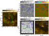 |
Fig. 1. Context images for regions studied in the present work taken on 2018 September 15. The AIA 171 Å image is giving an overview of the coronal structures in and around the studied regions (a). The contours (white lines) outline the boundaries of the coronal holes determined from the AIA 193 Å image. The region enclosed by the rectangle (green lines) is zoomed-in in panels b–e. The region of interest seen with HMI magnetic features (b), AIA 171 Å filtered (10−30 min) image (c), NVST Hα − 0.6 Å image (d) and AIA 171 Å image (e) is shown. The rectangles (blue lines) in panels b–e mark the network regions where coronal plumes are clearly seen. The green dotted lines in panel d mark two full and clear network regions. See animation online. |
3. Data analyses and results
In the Hα images, jets appear as dark features. In Fig. 1 and the associated animation, we can see that Hα jets are abundant in the network regions. To identify these jets, we upgraded the automatic algorithm that was described in Paper I; in addition, some key definitions are given in Huang et al. (2017). We note that “local peaks”, as defined in Huang et al. (2017), are replaced by the term “local trough”; in other words, we must multiply the Hα intensity by −1 to identify “local peaks”. In practical operations, we trace them from their bases to the top to obtain their full trajectories and then deduce their lifetimes and speeds.
3.1. Statistics of Hα jets
By applying the automatic algorithm on the full field-of-view, we identified and traced 1320 Hα jets during the observing period of time. We then obtained statistics on their lifetimes, heights, and speeds. Figure 2 shows the distributions of these properties. We obtained an average lifetime of 75.38 ± 33.08 s, an average height of 2.67 ± 1.03 Mm, and an average ascending velocity of 65.60 ± 42.59 km s−1. In the speed regime, 44% of Hα jets fall in the range between 10 km s−1 and 50 km s−1. These are consistent with the values found by Pasachoff et al. (2009), and this group of Hα jets is likely triggered by shocks (Hollweg 1982) or leakage from p-modes (De Pontieu et al. 2004). In particular, about 40% of Hα jets are in the range of 50−100 km s−1, which is in accord with typical values for Type II spicules, and about 16% of Hα jets have speeds higher than 100 km s−1, of which those with speeds of more than 150 km s−1 account for about 5%. Such high velocities are in good agreement with those reported for Type II spicules off the limb (e.g., De Pontieu et al. 2011, 2017; Martínez-Sykora et al. 2017). In the observations, we also find plenty of Hα jets moving up to the highest point, then disappearing. We also find that quite a few Hα jets undergo obvious swaying motions, but it is not easy to measure their periods because the lifetime of jets is too short to follow a complete cycle. Given the lack of spectroscopic observations, the torsional motions could be not identified.
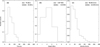 |
Fig. 2. Normalized distributions of the lifetimes (a), heights (b) and speeds (c) of the Hα jets identified and tracked in the whole field-of-view. The values following to “ave” and “stddev” are the average values and standard deviations of the corresponding parameters, respectively. |
From Fig. 1d, there are numerous Hα jets in the network regions. We select two full and clear network regions (see green-dashed lines) in Fig. 1d and count the number of Hα jets as shown in Fig. 3. The number of Hα jets is ∼58 per network region at any given time, which is consistent with reported spicules in previous studies (e.g., Lynch et al. 1973; Moore et al. 2011). Based on the similarities in terms of lifetime, speed, height, spatial extent, location near network, and birthrate, we suggest that the above analyzed Hα jets are extremely similar to spicules.
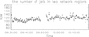 |
Fig. 3. Variation of the number of the Hα jets identified in two network regions as marked in Fig. 1d. The data around 09:50:00 have been removed due to bad observing conditions. |
3.2. Hα jets in the roots of coronal plumes
In Fig. 1, we see that plumes (plume-like features) are rooted in the regions of R1–R5, whereas they are hardly seen in other regions as determined from the AIA 171 Å images. We can also clearly see the coronal bright points in R1–R5. In the Hα images, we find 373 Hα jets rooted in R1–R5 and 947 rooted in the rest regions. In Fig. 4, we compare the statistics of Hα jets rooted in two kinds of regions. The normalized distributions of the lifetimes in Hα jets in these two regions are almost identical. The most significant differences are shown in the distributions of heights and speeds. Despite the fact that the distributions of each parameter from two different regions are largely overlapping, the distributions of heights and speeds from regions rich in coronal plumes (R1–R5) bias toward higher and faster wings than those from regions that are poor in coronal plumes. Specifically, Hα jets in R1–R5 have heights averaging 3.01 ± 1.07 Mm and speeds averaging 81.2 ± 48.3 km s−1. In contrast, the average height and speed of the Hα jets rooted in other regions poor in coronal plumes are 2.48 ± 0.95 Mm and 56.9 ± 36.3 km s−1, respectively.
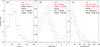 |
Fig. 4. Normalized distributions of the properties of (a) lifetimes, (b) heights, and (c) velocities of the Hα jets identified and tracked in the regions of R1–R5 (red lines) and the rest of the regions (black lines). The values following to “ave” and “stddev” are the average values and standard deviations of the corresponding parameters, respectively. |
Our study in Paper I shows that transition region network jets in the footpoints of coronal plumes also tend to be more dynamic (higher and faster) than those in other regions. Together with the consistent results found here in terms of the Hα jets, we may come to have two hypotheses: (1) a cascade effect might exist in these phenomena in which dynamic Hα jets power network jets and, subsequently, dynamic network jets power coronal plumes; (2) alternatively, high speed Hα jets, network jets and coronal plumes are three different counterparts of the same physical processes (e.g., compression of magnetic elements, Wang et al. 2016). A particular phenomenon consisting of multi-thermal structures is quite common in coronal dynamics with more rapid evolution, such as coronal jets (e.g., Sterling et al. 2015; Shen et al. 2017; Huang et al. 2018a, 2020), flaring events (e.g., Huang et al. 2014, 2018b; Wei et al. 2020), and coronal bright points (e.g., Madjarska et al. 2012; Huang 2018) – apart from relatively static events such as coronal plumes.
3.3. Hα jets and PDs in coronal plumes
In order to trace the PDs, we applied the simple bandpass filter on the AIA 171 Å images. We filter out the signals with the period shorter than 10 min and longer than 30 min. The detailed method is described in Jiao et al. (2015), while the results are shown in Fig. 1c. In the associated animation of Fig. 1, the PDs in R1–R5 can be clearly seen. Since the artificial periodicity near the cutoff periods might be introduced artificially (Auchère et al. 2016; Kayshap et al. 2020), we manually chose and further analyzed those PDs also showing discernible signals in the original images. We further investigated in detail the connection between the PDs and the Hα jets in their footpoint regions, and an example is given in Fig. 5. From Figs. 5A and B and the associated animations, we find that the footpoints of Hα jets and PDs are rooted in the same region, and the directions of their extensions are consistent with one another. For this reason, we believe that some Hα jets and PDs might share the same magnetic flux tubes. Figure 5C shows an time-distant diagram along the PDs (see yellow arrow in Fig. 5A). The blue-dashed lines mark the locations of PDs. Figures 5D and E display the maximum height and ascending speed of the Hα jets along the same path as the PDs observed at different time. Combined the panels C–E, we find that there is always a Hα jet appearing before presence of a PD and also having the same orientation as that of the PD (denoted by red arrows in panels D/E). We also notice that many Hα jets are rooted in the footpoints of PDs but not all of them are followed by PDs. Thus, an obvious question arises regarding what kind of Hα jets are associated with PDs. In Figs. 5D and E, for the same series of PDs, we can see that the Hα jets appear to be higher or faster before the PDs appear. For the series of PDs shown in Fig. 5, the Hα jets appearing just before PDs have an average height of 3.5 Mm and an average ascending velocity of 91.2 km s−1, in contrast to 3.0 Mm and 73.9 km s−1 for those appearing at other times. This seems as though the Hα jets corresponding to the PDs are more dynamic than those that not associated with PDs. To confirm this, we investigated all PDs identified in R1–R5, which include six series of them in total. In these PDs, we trace 29 associated Hα jets and show the histograms of their lifetimes, heights, and speeds in Fig. 6. Although the average height and speed values of these Hα jets do significantly vary from those rooted with coronal plumes, we can see that the almost all (except one) Hα jets followed by PDs have speeds of about or more than 50 km s−1. This implies that only those chromospheric jets with speeds of ≳50 km s−1 can go on to become associated with the given PDs. This conclusion, however, requires further observational, theoretical, or numerical investigations. The average lifetime of these Hα jets is significantly greater, but this is mainly due to the small sample set given that there are four with lifetimes greater than 200 s.
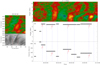 |
Fig. 5. Case analysis of the relationship between propagating disturbances (PDs) and Hα jet. Snapshot showing the connection between Hα jets in the NVST Hα − 0.6 Å (B) and PDs in the filtered AIA 171 Å (A). The yellow arrow outlines the structures of PDs determined from panel A, while the blue arrow represents the associated Hα jets from panel B. Time-slice images of the PD is shown in panel C. The blue lines mark the locations of PDs. Panel D and E: maximum height and ascending velocity of the Hα jets which exist in the footpoint of the given PD. Those denoted by the red arrows are those presented prior to the PD. See animation online. |
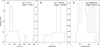 |
Fig. 6. Normalized distributions of the lifetimes (a), heights (b), and velocities (c) of the Hα jets that have a response from the PDs. |
We further selected a cluster of Hα jets existed in the vicinity of PDs (see between two red-dashed lines of Fig. 5B) and analyzed their dynamics when the PDs appear. We compared the average height and speed of the Hα jets when PDs are shown and when not shown. We find that heights and speeds of the groups of Hα jets with PDs are greater than those of Hα jets not associated with PDs. The Hα jets associated with PDs have heights averaging at 3.47 ± 0.06 Mm, and speeds averaging at 91.2 ± 32.8 km s−1. In contrast, the average height and speed of the Hα jets not associated with PDs are 3.06 ± 0.67 Mm and 73.4 ± 35.6 km s−1, respectively. Since the cross-section of a PD is much wider than a single Hα jet, it is difficult to associate a particular jet to the PD. Therefore, it remains possible that PDs are proceeded by a set of Hα jets, rather than a single one.
3.4. Relation between Hα jets and a coronal jet
Wang (1998) suggested that macrospicules seen in Hα jets and He II 304 jets are also direct manifestations of magnetic reconnection. Given that magnetic reconnection can trigger coronal jets, we investigate whether Hα jets have any connection with a faint coronal jet or not. In Fig. 7 and the associated animation, we show the evolution of the coronal jet observed in AIA 171 Å and the Hα jets rooted in the same region. From Fig. 7A, we can see that a coronal jet exists on the side of the footpoint of a coronal loop. In the animation, we clearly see that the loop expands from the bright base and form a blowout coronal jet at 09:50:28 UT, which can reach a height of about 9 Mm. In Fig. 7C, the blue-dashed lines mark the location of the coronal jet, whose speed is about 158 km s−1. We also find that a Hα jet blows up from the footpoints of the loops at 09:48:30 UT, just before initiation of the coronal jet (see Fig. 7B). The development of the Hα jet is fully consistent with that of the coronal jet, including their spatial extensions and directions. This Hα jet has a height of about 2.3 Mm and a rising speed of about 180 km s−1. The speed of the Hα jet is similar to that of the coronal jet. Therefore, we suggest that the coronal jets might be seen as the extension of part of Hα jets. Unfortunately, this coronal jet is the only such case found in the present observations. Subsequent statistical studies are required to confirm our conclusion.
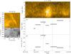 |
Fig. 7. Case analysis of the relationship between coronal jet and Hα jet. Snapshot showing the connection between Hα jets in the NVST Hα − 0.6 Å (B) and coronal jet in the AIA 171 Å (A). The yellow arrow outlines the structures of coronal jet determined from panel A, while the blue arrow represents the Hα jets from panel B. Time-slice images of the coronal jet is shown in panel C, the velocity is 158 km s−1. Panels D and E: maximum height and ascending velocity of the Hα jets that exist in the footpoint of the given coronal jet (see those denoted by the red arrows). The blue dashed lines indicate the location of the coronal jet. See animation online. |
4. Discussion
In Paper I, we studied the relation between transition region network jets and coronal plumes. In the present work, we focus on chromospheric jet-like features observed in Hα − 0.6 Å, namely Hα jets. In agreement with Paper I, we found that the network regions where the coronal counterparts are active with coronal bright points and plumes tend to produce Hα jets with more dynamic characteristics (i.e., larger heights and faster speeds) than those from the other network regions. Given that Hα jets, network jets and coronal plumes may be associated with magnetic reconnection, it is possible that the energy produced by magnetic activities could be transferred from the fine structures in the low solar atmosphere to those in the corona.
In this paper, we find a few examples that Hα jets have a one-to-one correspondence with PDs in spatial and temporal. The Hα jets associated with PDs are usually faster and higher than the others. Furthermore, Wang et al. (1998) found that He II 304 Å jets are always associated with Hα jets, but not all the Hα jets are associated with He II 304 Å jets. We find that the faster and higher Hα jets have a certain relationship with coronal jets. It is possible that only certain parts of Hα jets that are more energetic can reach the low corona and can also be seen in He II 304 Å. We attempt to find an answer to why the Hα jets are higher and faster at the roots of coronal plumes and jets and we discuss the possible mechanisms below.
The first interpretation is associated with the generation of transverse wave induced Kelvin-Helmholtz instability (KHi) in Hα jets. It has been proved that chromospheric jets usually accompany transverse motions with amplitudes up to 10 − 25 km s−1 (De Pontieu et al. 2007c), which are generally interpreted as kink waves (He et al. 2009). Such waves are possible to induce the KHi due to velocity shear between magnetic structures and background medium (e.g., Terradas et al. 2008; Antolin et al. 2018, etc.). Antolin et al. (2018) considered the KHi induced by kink motions and attributed some observational properties of spicules to the development of KHi eddies. The small spatial structures induced by the KHi can help the dissipation of wave energy, thus playing an important role in understanding temperature increase of magnetic structures (e.g., Guo et al. 2019; Karampelas et al. 2019). In addition, Lau & Liu (1980) pointed out that if a longitudinal flow exceeds a criterion, the magnetized plasma is unstable. With the IRIS observations, Li et al. (2018a) found that the KHi could develop due to the strong shear (more than 204 km s−1) between two blowout jets. In the case of kink waves with longitudinal flows, the criterion for developing the KHi has been discussed in many works in the literature (e.g., Andries & Goossens 2001; Zhelyazkov et al. 2016; Li et al. 2018a). The threshold was derived by Andries & Goossens (2001) from eigen-mode analysis in a cylindrical model. It reads  , where U (VAi) represents the flow (Alfvén) speed inside a jet, while Bi(ρi) and Be(ρe) are the magnetic field strength (density) in a jet and the ambient region, respectively. In spicules, the density and magnetic field of a chromospheric jet is about 3 × 1010 cm−3 and 40 G, respectively. We assume those for the ambient regions are 1 × 109 cm−3 and 10 G (see Tsiropoula et al. 2012; Sterling 2000; Centeno et al. 2010, and references therein). Generally, the Alfvén speed in the choromosphere is 40 km s−1 (De Pontieu et al. 2007c), indicating that the KHi can be induced in spicules when the upflow speed exceeds 98 km s−1. Furthermore, Zhelyazkov et al. (2016) studied the propagating of kink waves in EUV jets in vertical magnetic tubes. They found that kink waves could become unstable when the flow velocity exceeds 112 km s−1. In Fig. 4, we can see that 28.4% Hα jets have a higher speed (more than 110 km s−1) in R1–R5, while only 8.3% Hα jets with such high speed in other regions. This means that in the aforementioned observations, the KHi is possible to develop in faster Hα jets in R1–R5. Due to the development of the KHi, it is possible for the faster Hα jets to dissipate energy into higher atmospheres. Moreover, Cavus & Kazkapan (2013) proposed that the KHi might be a mechanism for the formation of magnetic reconnection. This means that the Hα jets with KHi might be capable of heating the corona. However, more detailed simulations should be considered in future studies to explore this possibility.
Another possible interpretation is the interaction strength among small-scale magnetic elements in the network region. For R1–R5, there are dominant network fields and some small-scale opposite-polarity fields in Fig. 1b. Wang et al. (2016) proposed that the convergence of the base flux could trigger coronal plumes. The interaction of magnetic flux concentrations with constantly weak fields could result in strong magnetic tension. The strong magnetic tension which is amplified and transported upward through ambipolar diffusion could produce numerical faster spicules (more than 100 km s−1) in the 2.5D simulation (Martínez-Sykora et al. 2017). In addition, as in the 2.5D numerical simulation, Ding et al. (2011) also showed that the stronger magnetic field could produce higher up-flow velocities. These simulations indicate that there is a great possibility for the presence of rapid jets in the network field with weak opposite magnetic elements and these jets might have coronal connection. Using high spatial-resolution and high time-cadence observations of the Goode Solar Telescope (GST, Goode et al. 2010; Cao et al. 2010), Samanta et al. (2019) provided observations from the photosphere to the chromosphere and the corona to support the notion that these chromospheric jets (∼50 km s−1) are driven by the interaction between strong network fields with small-scale opposite-polarity fields that have a good coronal connection. Thanks to the order-of-magnitude estimation of energies, the authors estimated that these spicules supply enough energy into the corona. The speeds of these jets are smaller than what is shown in our results because the FOV in Samanta et al. (2019) is close to the center of disk. With respect to the relation between the chromospheric jets and coronal activities, the mixed-polarity magnetic fields could result in the shuffling and further braiding of small-scale magnetic field lines, which produce magnetic reconnection at braiding boundaries and power the corona. In the same vein, Li et al. (2018b) proposed that the dissipation of electric currents that is due to the effect of small-scale weak magnetic activities (including spicules) could effectively heat the corona at low heights. In addition, Priest et al. (2002) showed that the formation and dissipation of current sheets along these separatrices (resulting from highly fragmented photospheric magnetic configurations) could be an important contribution to coronal heating. This means that the activities of mixed-polarity on small scales might have enough power to fuel coronal activities. In Fig. 1d, we see that Hα jets are located near the dominant network fields, but the lower resolution of magnetic fields measurements affect the detection of weak magnetic elements at the footpoints of Hα jets. Further studies using high spatial-temporal resolution observations of the photosphere – such as the Goode Solar Telescope (GST), the forthcoming Daniel K. Inouye Solar Telescope (DKIST), and the planned Chinese Advanced Solar Observatories–Ground-based (ASO-G) – is expected to shed more light on this topic.
The analyses presented in this work show that Hα jets with coronal responses tend to be higher and faster. The question of whether there is a critical height and speed for a Hα jet having coronal response should be investigated both theoretically and observationally. As discussed above, it may lead to different possibilities based on the various aforementioned mechanisms. Based on the present observations, we cannot find evidence of KHi due to the spatial and temporal resolutions. The HMI magnetograms clearly show that a number of small-scale magnetic elements appear and disappear in the footpoints of these Hα jets (see the animation associated with Fig. 1). Although the observed region is pretty much closed to the limb, the observations still give a hint of a degree of magnetic dynamics. Therefore, with the present observations, the scenario that appears more favorable is that of a more powerful interaction between small-scale magnetic elements tending to generate more dynamic phenomena. However, the KHi scenario cannot be ruled out within the present circumstances. In the near future, we will carry out an in-depth study on how much the initial energy of chromospheric jets is required to elicit coronal responses based on the above-mentioned mechanism.
5. Conclusions
In this paper, we analyze observations taken by the 1-m New Vacuum Solar Telescope at the Hα − 0.6 Å passband. Thanks to the higher spatial and temporal resolution of the data, we were able to trace the evolutions of Hα jets over time. Using an upgraded automated detection algorithm, we carried out a statistical study of Hα jets. Using the algorithm, we identified and traced 1320 Hα jets in the data set. We found that the average lifetime, height and ascending speed of the Hα jets are 75.38 s, 2.67 Mm, 65.60 km s−1, respectively. These characteristics are in good agreement with those of Type II spicules. In addition, we find that the Hα jets occur in network regions where magnetic concentrations are present. We believe that the Hα jets correspond to spicules or the on-disk counterparts of spicules.
We found that Hα jets rooted in the footpoint regions of coronal plumes have an average lifetime of 76.1 ± 35.0 s, an average height of 3.01 ± 1.07 Mm, and an average ascending velocity of 81.2 ± 48.3 km s−1. While the Hα jets in the rest regions exhibit an average lifetime of 75.0 ± 32.0 s, an average height of 2.48 ± 0.95 Mm, and an average ascending velocity of 56.9 ± 36.3 km s−1, these results show that the Hα jets associated with coronal plumes are, on average, higher and more dynamic than those that are not associated with coronal plumes. Furthermore, we considered whether these jets can possibly provide enough energy to sustain a coronal plume. In the corona, the radiation cooling time is expressed as  in the corona (Aschwanden & Terradas 2008), taking in typical parameters of corona and plumes, where the radiative loss rate Λ0 ∼ 10−17.73 ergs cm−3, a temperature of T ∼ 1.0 MK and density of n ∼ 109 cm−3, then we find the radiation cooling time scale is on the order of 1000 s. While the Hα jets in the footpoint of a plume studied here repeatedly present a timescale of about 80 s – much less than the radiation cooling time in the corona, suggesting that the Hα jets may provide energy continuously to sustain the coronal plumes.
To determine exactly what type of Hα jets might be linked to coronal activities, we further investigated the connection between Hα jets and the PDs in plumes. We find that there are always Hα jets appearing before the initiation of PDs and extending in the same directions of the PDs. Almost all of these jets (28 out of 29) have speeds ≳50 km s−1; thus, we suggest that only those Hα jets exceeding a certain velocity can be precursors of PDs.
A fade coronal jet with a speed of about 160 km s−1 was also observed. We find that this coronal jet is accompanied by a Hα jet that has a speed comparable to that of the coronal jet, suggesting that the coronal jet might be the extension of part of the Hα jets.
In agreement with Paper I, the present studies confirm that small-scale jet-like features in the solar lower atmosphere can be directly connected to coronal activities. Given that most Hα jets observed here are likely spicules in the chromosphere, we suggest that Hα jets, when they are dynamic to a certain extent, can sufficiently power the corona. In combining these findings with the results shown in Paper I, we suggest that spicule-like features in the chromosphere, transition region network jets, and ray-like features in the corona are coherent phenomena are important vehicles for cycling energy and mass in the solar atmosphere.
Movies
Movie 1 associated with Fig. 1 (fov) Access Supplementary Material
Movie 2 associated with Fig. 5 (pd_hajet) Access Supplementary Material
Movie 3 associated with Fig. 7 (coronaljet_hajet) Access Supplementary Material
Acknowledgments
We are grateful to the anonymous reviewer for the constructive comments and suggestions. L.X. and Y.Q. are supported by National Natural Science Foundation of China (NSFC) under contract No. 41974201. Z.H. thanks financial supports from NSFC under contract No. U1831112 and the Young Scholar Program of Shandong University, Weihai (2017WHWLJH07). H.F. is supported by NSFC contract No. U1931105. W.L. is supported by NSFC contract No. U1931122. M.S. is supported by NSFC contract No. 41627806. We would like to thank the NVST operation team for their hospitality during the observing campaign and preparation of the data. The data used are also courtesy of NASA/SDO, the AIA and HMI teams and JSOC.
References
- Andries, J., & Goossens, M. 2001, A&A, 368, 1083 [NASA ADS] [CrossRef] [EDP Sciences] [Google Scholar]
- Antolin, P., Schmit, D., Pereira, T. M. D., De Pontieu, B., & De Moortel, I. 2018, ApJ, 856, 44 [Google Scholar]
- Aschwanden, M. J., & Terradas, J. 2008, ApJ, 686, L127 [NASA ADS] [CrossRef] [Google Scholar]
- Auchère, F., Froment, C., Bocchialini, K., Buchlin, E., & Solomon, J. 2016, ApJ, 825, 110 [Google Scholar]
- Beckers, J. M. 1968, Sol. Phys., 3, 367 [NASA ADS] [Google Scholar]
- Cao, W., Gorceix, N., Coulter, R., et al. 2010, Astron. Nachr., 331, 636 [Google Scholar]
- Cavus, H., & Kazkapan, D. 2013, New Astron., 25, 89 [NASA ADS] [CrossRef] [Google Scholar]
- Centeno, R., Trujillo Bueno, J., & Asensio Ramos, A. 2010, ApJ, 708, 1579 [NASA ADS] [CrossRef] [Google Scholar]
- De Pontieu, B., Erdélyi, R., & James, S. P. 2004, Nature, 430, 536 [Google Scholar]
- De Pontieu, B., Hansteen, V. H., Rouppe van der Voort, L., van Noort, M., & Carlsson, M. 2007a, ApJ, 655, 624 [Google Scholar]
- De Pontieu, B., McIntosh, S., Hansteen, V. H., et al. 2007b, PASJ, 59, S655 [Google Scholar]
- De Pontieu, B., McIntosh, S. W., Carlsson, M., et al. 2007c, Science, 318, 1574 [Google Scholar]
- De Pontieu, B., Hansteen, V. H., Rouppe van der Voort, L., van Noort, M., & Carlsson, M. 2007d, in The Physics of Chromospheric Plasmas, eds. P. Heinzel, I. Dorotovič, & R. J. Rutten, ASP Conf. Ser., 368, 65 [Google Scholar]
- De Pontieu, B., McIntosh, S. W., Carlsson, M., et al. 2011, Science, 331, 55 [Google Scholar]
- De Pontieu, B., Title, A., & Carlsson, M. 2014, Science, 346, 315 [NASA ADS] [CrossRef] [Google Scholar]
- De Pontieu, B., Martínez-Sykora, J., & Chintzoglou, G. 2017, ApJ, 849, L7 [Google Scholar]
- DeForest, C. E., & Gurman, J. B. 1998, ApJ, 501, L217 [NASA ADS] [CrossRef] [Google Scholar]
- Ding, J. Y., Madjarska, M. S., Doyle, J. G., et al. 2011, A&A, 535, A95 [NASA ADS] [CrossRef] [EDP Sciences] [Google Scholar]
- Fu, H., Xia, L., Li, B., et al. 2014, ApJ, 794, 109 [NASA ADS] [CrossRef] [Google Scholar]
- Goode, P. R., Coulter, R., Gorceix, N., Yurchyshyn, V., & Cao, W. 2010, Astron. Nachr., 331, 620 [NASA ADS] [CrossRef] [Google Scholar]
- Guo, M., Van Doorsselaere, T., Karampelas, K., et al. 2019, ApJ, 870, 55 [Google Scholar]
- Hansteen, V. H., De Pontieu, B., Rouppe van der Voort, L., van Noort, M., & Carlsson, M. 2006, ApJ, 647, L73 [Google Scholar]
- He, J., Marsch, E., Tu, C., & Tian, H. 2009, ApJ, 705, L217 [NASA ADS] [CrossRef] [Google Scholar]
- Heggland, L., De Pontieu, B., & Hansteen, V. H. 2007, ApJ, 666, 1277 [Google Scholar]
- Heggland, L., Hansteen, V. H., De Pontieu, B., & Carlsson, M. 2011, ApJ, 743, 142 [CrossRef] [Google Scholar]
- Hollweg, J. V. 1982, ApJ, 257, 345 [NASA ADS] [CrossRef] [Google Scholar]
- Huang, Z. 2018, ApJ, 869, 175 [NASA ADS] [CrossRef] [Google Scholar]
- Huang, Z., Madjarska, M. S., Koleva, K., et al. 2014, A&A, 566, A148 [NASA ADS] [CrossRef] [EDP Sciences] [Google Scholar]
- Huang, Z., Madjarska, M. S., Scullion, E. M., et al. 2017, MNRAS, 464, 1753 [NASA ADS] [CrossRef] [Google Scholar]
- Huang, Z., Xia, L., Nelson, C. J., et al. 2018a, ApJ, 854, 80 [NASA ADS] [CrossRef] [Google Scholar]
- Huang, Z., Mou, C., Fu, H., et al. 2018b, ApJ, 853, L26 [NASA ADS] [CrossRef] [Google Scholar]
- Huang, Z., Zhang, Q., Xia, L., et al. 2020, ApJ, 897, 113 [Google Scholar]
- Huang, Z., Zhang, Q., Xia, L., et al. 2021, Sol. Phys., 296, 22 [NASA ADS] [CrossRef] [Google Scholar]
- Jiao, F., Xia, L., Li, B., et al. 2015, ApJ, 809, L17 [NASA ADS] [CrossRef] [Google Scholar]
- Karampelas, K., Van Doorsselaere, T., & Guo, M. 2019, A&A, 623, A53 [NASA ADS] [CrossRef] [EDP Sciences] [Google Scholar]
- Kayshap, P., Srivastava, A. K., Tiwari, S. K., Jelínek, P., & Mathioudakis, M. 2020, A&A, 634, A63 [NASA ADS] [CrossRef] [EDP Sciences] [Google Scholar]
- Krishna Prasad, S., Banerjee, D., & Gupta, G. R. 2011, A&A, 528, L4 [NASA ADS] [CrossRef] [EDP Sciences] [Google Scholar]
- Langangen, Ø., De Pontieu, B., Carlsson, M., et al. 2008, ApJ, 679, L167 [Google Scholar]
- Lau, Y. Y., & Liu, C. S. 1980, Phys. Fluids, 23, 939 [CrossRef] [Google Scholar]
- Lemen, J. R., Title, A. M., Akin, D. J., et al. 2012, Sol. Phys., 275, 17 [Google Scholar]
- Li, X., Zhang, J., Yang, S., Hou, Y., & Erdélyi, R. 2018a, Sci. Rep., 8, 8136 [CrossRef] [Google Scholar]
- Li, K. J., Xu, J. C., & Feng, W. 2018b, ApJS, 237, 7 [NASA ADS] [CrossRef] [Google Scholar]
- Liu, Z., Xu, J., Gu, B.-Z., et al. 2014, Res. Astron. Astrophys., 14, 705 [Google Scholar]
- Liu, J., McIntosh, S. W., De Moortel, I., & Wang, Y. 2015, ApJ, 806, 273 [NASA ADS] [CrossRef] [Google Scholar]
- Lynch, D. K., Beckers, J. M., & Dunn, R. B. 1973, Sol. Phys., 30, 63 [NASA ADS] [CrossRef] [Google Scholar]
- Madjarska, M. S., Huang, Z., Doyle, J. G., & Subramanian, S. 2012, A&A, 545, A67 [NASA ADS] [CrossRef] [EDP Sciences] [Google Scholar]
- Martínez-Sykora, J., De Pontieu, B., Hansteen, V. H., et al. 2017, Science, 356, 1269 [Google Scholar]
- McIntosh, S. W., Innes, D. E., de Pontieu, B., & Leamon, R. J. 2010, A&A, 510, L2 [NASA ADS] [CrossRef] [EDP Sciences] [Google Scholar]
- Moore, R. L., Sterling, A. C., Cirtain, J. W., & Falconer, D. A. 2011, ApJ, 731, L18 [NASA ADS] [CrossRef] [Google Scholar]
- Panesar, N. K., Sterling, A. C., Moore, R. L., et al. 2018, ApJ, 868, L27 [CrossRef] [Google Scholar]
- Pant, V., Dolla, L., Mazumder, R., et al. 2015, ApJ, 807, 71 [NASA ADS] [CrossRef] [Google Scholar]
- Pasachoff, J. M., Jacobson, W. A., & Sterling, A. C. 2009, Sol. Phys., 260, 59 [Google Scholar]
- Pesnell, W. D., Thompson, B. J., & Chamberlin, P. C. 2012, Sol. Phys., 275, 3 [Google Scholar]
- Priest, E. R., Heyvaerts, J. F., & Title, A. M. 2002, ApJ, 576, 533 [NASA ADS] [CrossRef] [Google Scholar]
- Qi, Y., Huang, Z., Xia, L., et al. 2019, Sol. Phys., 294, 92 [NASA ADS] [CrossRef] [Google Scholar]
- Raouafi, N. E., & Stenborg, G. 2014, ApJ, 787, 118 [NASA ADS] [CrossRef] [Google Scholar]
- Raouafi, N. E., Petrie, G. J. D., Norton, A. A., Henney, C. J., & Solanki, S. K. 2008, ApJ, 682, L137 [NASA ADS] [CrossRef] [Google Scholar]
- Raouafi, N. E., Patsourakos, S., Pariat, E., et al. 2016, Space Sci. Rev., 201, 1 [Google Scholar]
- Rouppe van der Voort, L. H. M., De Pontieu, B., Hansteen, V. H., Carlsson, M., & van Noort, M. 2007, ApJ, 660, L169 [Google Scholar]
- Rouppe van der Voort, L., Leenaarts, J., de Pontieu, B., Carlsson, M., & Vissers, G. 2009, ApJ, 705, 272 [Google Scholar]
- Rouppe van der Voort, L., De Pontieu, B., Pereira, T. M. D., Carlsson, M., & Hansteen, V. 2015, ApJ, 799, L3 [Google Scholar]
- Samanta, T., Tian, H., Yurchyshyn, V., et al. 2019, Science, 366, 890 [NASA ADS] [CrossRef] [Google Scholar]
- Schou, J., Scherrer, P. H., Bush, R. I., et al. 2012, Sol. Phys., 275, 229 [Google Scholar]
- Sekse, D. H., Rouppe van der Voort, L., & De Pontieu, B. 2012, ApJ, 752, 108 [Google Scholar]
- Sekse, D. H., Rouppe van der Voort, L., & De Pontieu, B. 2013, ApJ, 764, 164 [Google Scholar]
- Shen, Y., Liu, Y. D., Su, J., Qu, Z., & Tian, Z. 2017, ApJ, 851, 67 [NASA ADS] [CrossRef] [Google Scholar]
- Sterling, A. C. 2000, Sol. Phys., 196, 79 [NASA ADS] [CrossRef] [Google Scholar]
- Sterling, A. C., Moore, R. L., Falconer, D. A., & Adams, M. 2015, Nature, 523, 437 [NASA ADS] [CrossRef] [Google Scholar]
- Terradas, J., Andries, J., Goossens, M., et al. 2008, ApJ, 687, L115 [Google Scholar]
- Tian, H., Tu, C., Marsch, E., He, J., & Kamio, S. 2010, ApJ, 709, L88 [NASA ADS] [CrossRef] [Google Scholar]
- Tian, H., McIntosh, S. W., Habbal, S. R., & He, J. 2011, ApJ, 736, 130 [NASA ADS] [CrossRef] [Google Scholar]
- Tian, H., DeLuca, E. E., Cranmer, S. R., et al. 2014, Science, 346, 1255711 [Google Scholar]
- Tsiropoula, G., Tziotziou, K., Kontogiannis, I., et al. 2012, Space Sci. Rev., 169, 181 [Google Scholar]
- Wang, H. 1998, ApJ, 509, 461 [NASA ADS] [CrossRef] [Google Scholar]
- Wang, Y. M., & Muglach, K. 2008, Sol. Phys., 249, 17 [NASA ADS] [CrossRef] [Google Scholar]
- Wang, Y. M., & Sheeley, N. R., Jr. 1995, ApJ, 452, 457 [NASA ADS] [CrossRef] [Google Scholar]
- Wang, Y. M., Sheeley, N. R., Dere, K. P., et al. 1997, ApJ, 484, L75 [NASA ADS] [CrossRef] [Google Scholar]
- Wang, H., Johannesson, A., Stage, M., Lee, C., & Zirin, H. 1998, Sol. Phys., 178, 55 [NASA ADS] [CrossRef] [Google Scholar]
- Wang, Y. M., Warren, H. P., & Muglach, K. 2016, ApJ, 818, 203 [NASA ADS] [CrossRef] [Google Scholar]
- Wei, H., Huang, Z., Hou, Z., et al. 2020, MNRAS, 498, L104 [NASA ADS] [CrossRef] [Google Scholar]
- Wilhelm, K., Abbo, L., Auchère, F., et al. 2011, A&ARv, 19, 35 [NASA ADS] [CrossRef] [Google Scholar]
- Xia, L. D., Marsch, E., & Curdt, W. 2003, A&A, 399, L5 [NASA ADS] [CrossRef] [EDP Sciences] [Google Scholar]
- Xia, L. D., Marsch, E., & Wilhelm, K. 2004, A&A, 424, 1025 [NASA ADS] [CrossRef] [EDP Sciences] [Google Scholar]
- Xiang, Y.-Y., Liu, Z., & Jin, Z.-Y. 2016, New Astron., 49, 8 [CrossRef] [Google Scholar]
- Yang, Y.-F., Qu, H.-X., Ji, K.-F., et al. 2015, Res. Astron. Astrophys., 15, 569 [CrossRef] [Google Scholar]
- Zhelyazkov, I., Chandra, R., & Srivastava, A. K. 2016, Ap&SS, 361, 51 [NASA ADS] [CrossRef] [Google Scholar]
All Figures
|
Fig. 1. Context images for regions studied in the present work taken on 2018 September 15. The AIA 171 Å image is giving an overview of the coronal structures in and around the studied regions (a). The contours (white lines) outline the boundaries of the coronal holes determined from the AIA 193 Å image. The region enclosed by the rectangle (green lines) is zoomed-in in panels b–e. The region of interest seen with HMI magnetic features (b), AIA 171 Å filtered (10−30 min) image (c), NVST Hα − 0.6 Å image (d) and AIA 171 Å image (e) is shown. The rectangles (blue lines) in panels b–e mark the network regions where coronal plumes are clearly seen. The green dotted lines in panel d mark two full and clear network regions. See animation online. |
| In the text | |
|
Fig. 2. Normalized distributions of the lifetimes (a), heights (b) and speeds (c) of the Hα jets identified and tracked in the whole field-of-view. The values following to “ave” and “stddev” are the average values and standard deviations of the corresponding parameters, respectively. |
| In the text | |
|
Fig. 3. Variation of the number of the Hα jets identified in two network regions as marked in Fig. 1d. The data around 09:50:00 have been removed due to bad observing conditions. |
| In the text | |
|
Fig. 4. Normalized distributions of the properties of (a) lifetimes, (b) heights, and (c) velocities of the Hα jets identified and tracked in the regions of R1–R5 (red lines) and the rest of the regions (black lines). The values following to “ave” and “stddev” are the average values and standard deviations of the corresponding parameters, respectively. |
| In the text | |
|
Fig. 5. Case analysis of the relationship between propagating disturbances (PDs) and Hα jet. Snapshot showing the connection between Hα jets in the NVST Hα − 0.6 Å (B) and PDs in the filtered AIA 171 Å (A). The yellow arrow outlines the structures of PDs determined from panel A, while the blue arrow represents the associated Hα jets from panel B. Time-slice images of the PD is shown in panel C. The blue lines mark the locations of PDs. Panel D and E: maximum height and ascending velocity of the Hα jets which exist in the footpoint of the given PD. Those denoted by the red arrows are those presented prior to the PD. See animation online. |
| In the text | |
|
Fig. 6. Normalized distributions of the lifetimes (a), heights (b), and velocities (c) of the Hα jets that have a response from the PDs. |
| In the text | |
|
Fig. 7. Case analysis of the relationship between coronal jet and Hα jet. Snapshot showing the connection between Hα jets in the NVST Hα − 0.6 Å (B) and coronal jet in the AIA 171 Å (A). The yellow arrow outlines the structures of coronal jet determined from panel A, while the blue arrow represents the Hα jets from panel B. Time-slice images of the coronal jet is shown in panel C, the velocity is 158 km s−1. Panels D and E: maximum height and ascending velocity of the Hα jets that exist in the footpoint of the given coronal jet (see those denoted by the red arrows). The blue dashed lines indicate the location of the coronal jet. See animation online. |
| In the text | |
Current usage metrics show cumulative count of Article Views (full-text article views including HTML views, PDF and ePub downloads, according to the available data) and Abstracts Views on Vision4Press platform.
Data correspond to usage on the plateform after 2015. The current usage metrics is available 48-96 hours after online publication and is updated daily on week days.
Initial download of the metrics may take a while.