| Issue |
A&A
Volume 657, January 2022
|
|
|---|---|---|
| Article Number | A103 | |
| Number of page(s) | 16 | |
| Section | Planets and planetary systems | |
| DOI | https://doi.org/10.1051/0004-6361/202141213 | |
| Published online | 19 January 2022 | |
Eviction-like resonances for satellite orbits
Application to Phobos, the main satellite of Mars
1
CIDMA, Departamento de Matemática, Universidade de Aveiro,
Campus de Santiago,
3810-193
Aveiro,
Portugal
e-mail: This email address is being protected from spambots. You need JavaScript enabled to view it.
2
CFisUC, Departamento de Física, Universidade de Coimbra,
3004-516
Coimbra,
Portugal
3
ASD, IMCCE-CNRS UMR8028, Observatoire de Paris, PSL Université,
77 Av. Denfert-Rochereau,
75014
Paris,
France
Received:
30
April
2021
Accepted:
13
October
2021
Abstract
The motion of a satellite can experience secular resonances between the precession frequencies of its orbit and the mean motion of the host planet around the star. Some of these resonances can significantly modify the eccentricity (evection resonance) and the inclination (eviction resonance) of the satellite. In this paper, we study in detail the secular resonances that can disturb the orbit of a satellite, in particular the eviction-like ones. Although the inclination is always disturbed while crossing one eviction-like resonance, capture can only occur when the semi-major axis is decreasing. This is, for instance, the case of Phobos, the largest satellite of Mars, that will cross some of these resonances in the future because its orbit is shrinking owing to tidal effects. We estimate the impact of resonance crossing in the orbit of the satellite, including the capture probabilities, as a function of several parameters, such as the eccentricity and the inclination of the satellite, and the obliquity of the planet. Finally, we use the method of the frequency map analysis to study the resonant dynamics based on stability maps, and we show that some of the secular resonances may overlap, which leads to chaotic motion for the inclination of the satellite.
Key words: celestial mechanics / planets and satellites: dynamical evolution and stability / planets and satellites: individual: Phobos
© ESO 2022
1 Introduction
The orbit of a satellite can give some hints as to its origin. If the satellite forms at the same time as its planet within an accretion disk, it is expected that the satellite is located in the equatorial plane of the planet in a nearly circular orbit (e.g., Batygin & Morbidelli 2020; Inderbitzi et al. 2020). If the satellite forms from a giant impact, the initial orbit is also expected to be equatorial, but it can be very eccentric (e.g., Canup & Asphaug 2001; Canup 2005). Finally, if the satellite is a captured object, its orbit is expected to be very eccentric as well and to present some inclination with respect to the planet’s equator (e.g., Agnor & Hamilton 2006; Nesvorný et al. 2007).
Tidal dissipation inside the planet and the satellite can significantly modify some orbital parameters, in particular the semi-major axis and the eccentricity. Tidal dissipation can also lead to variations in the inclination of the satellite, although these variations are weak and often negligible (e.g., Lambeck 1979; Szeto 1983). Therefore, the inclination is not modified by tides much and, contrary to the semi-major axis and the eccentricity, it can be used to distinguish between the capture scenario and other formation scenarios. Nevertheless, secular resonances can also modify the orbital parameters of the satellite. For instance, in the case of Phobos, the main satellite of Mars, Yoder (1982) noted that during its evolution, the satellite crossed several resonances which have successively excited its eccentricity. Therefore, the current value cannot be considered simply as the result of the tidal dissipation of the primordial eccentricity. The evection resonance, which corresponds to an interaction between the secular precession of the pericenter of the satellite and the orbital mean motion of the planet, can also lead to a variation in the eccentricity of the satellite (e.g., Touma & Wisdom 1998). This effect is stronger when capture in the evection resonance occurs, although this is only possible if the semi-major axis is increasing, which is, for instance, the case for the early Moon.
There are also resonances that are able to modify the inclination of a satellite, corresponding to an interaction between the precession of the node of its orbit and the orbital mean motion of the planet. Touma & Wisdom (1998) noted that the early Moon could also have been temporarily captured in a resonance of this kind, which they called “eviction” (just after it escapes from the evection resonance). This temporary capture can lead to an increase of around ten degrees in the inclination of the early Moon with respect to the Earth’s equator, which may explain the current mutual inclination of the lunar orbit of about five degrees. The capture of the Moon in the eviction resonance is only possible if the semi-major axis is decreasing and if the eccentricity is sufficiently high. Touma & Wisdom (1998) also noted that if the Moon encounters the eviction resonance while the semi-major axis increases, it would not be captured, but it could nevertheless lead to a one-time increase in the inclination, provided that the eccentricity is high enough.
As the semi-major axis of Phobos is currently decreasing due to tides (e.g., Jacobson & Lainey 2014), it can also be captured in eviction-like resonances. Indeed, Yokoyama (2002) showed that Phobos will encounter two of these resonances in the near future, which may significantly increase its equatorial inclination. Contrary to the original eviction resonance described by Touma & Wisdom (1998), capture in these two resonances is possible for zero eccentricity. In order to study these resonances, Yokoyama (2002) considered a system of three bodies with the Sun, Mars, and a massless satellite, where the orbit of Mars is circular. For this system, Yokoyama (2002) numerically integrated the equations of the satellite obtained from an averaged Hamiltonian, and noted that the capture probabilities in these resonances strongly depend on the Martian obliquity. When capture does not occur, the resonance crossing can still lead to a sudden variation in the inclination. The capture probability in one resonance is almost certain if the obliquity of Mars is higher than 20 degrees. Similar results for this resonance are observed in the case where the precession of the Martian equator, the obliquity variations (Yokoyama 2002), or the planetary perturbations on Mars are considered (Yokoyama et al. 2005). For the other resonance, which occurs almost simultaneously with the evection resonance, Yokoyama (2002) numerically observed that capture is possible with the resonantHamiltonian, but becomes impossible with the total Hamiltonian. Yokoyama (2002) then concluded that the impossibility of the capture is due to the interaction between the two resonances. Yokoyama et al. (2005) considered a more complete model including the Mars’ eccentricity, and observed that it increases the interaction with the evection resonance and its effects.
In this paper, we revisit the secular resonances between the orbit of the satellite and the mean motion of the planet. We focus on those that are suitable to excite the inclination of the satellite (eviction-like), since the inclination can be used to put constrains on the formation scenarios. The aim of the paper is to estimate what can be the effects of such resonances on the orbital evolution of a satellite. For this, we evaluate precisely the capture probabilities of a satellite in these resonances, and the variations in orbital parameters due to their crossings in the case where the capture fails. We also study the interaction with the evection resonance observed by Yokoyama (2002) to determinate in which extent it influences the dynamics of a satellite and determine the exact mechanism behind this excitation.
In Sect. 2, we first derive a secular model that is suitable to describe the dynamics of a massless satellite of a rigid planet perturbed by the host star. In Sect. 3, we identify all the possible secular resonances when the planet is in a circular orbit around the star and its equator uniformly precesses with constant obliquity. In Sect. 4, we study in detail with analytical models the main eviction-like resonances that may significantly modify the inclination of the satellite. In Sect. 5, we study the interaction of neighbor secular resonances using frequency map analysis. In Sect. 6, we apply our model to the future evolution of Phobos and numerically estimate the capture probabilities in resonancefor different values of the eccentricity and obliquity. Finally, we discuss our results in Sect. 7.
2 Model
We consider a star orbited by a planet and a satellite, with masses m0, m1 and m, respectively. The star and the satellite are considered point masses. The planet is a rigid body with moments of inertia A ≤ B ≤ C, and rotational angular momentum S.
The variables (a, e, i, λ, ϖ, Ω) denote respectively the semi-major axis, the eccentricity, the inclination with respect to a reference plane, the mean longitude (λ = ϖ + M, with M the mean anomaly), the longitude of the pericenter (ϖ = ω + Ω, with ω the argument of the pericenter), and the longitude of the ascending node of the orbit of the satellite around the planet. The same variables with a subscript 1 are used for the orbit of the planet around the star, that we name for simplicity, the ecliptic.
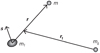 |
Fig. 1 Jacobi coordinates, where r is the position of m relative to m1 (satellite orbit), and r1 is the position of the center of mass of m and m1 relative to m0 (planet orbit). The planet is a rigid body, where S is the rotational angular momentum. |
2.1 Secular Hamiltonian
We let  be the barycentric canonical variables with Ri the position vector with respect to the barycenter of the system, and
  the conjugate momenta (i = 0, 1, for the star, and planet, respectively, and we do not use subscripts for the variables of the satellite). We perform a canonical change into Jacobi variables
  as r0 = R0, r1 = δR + (1 − δ)R1 −R0, and r = R −R1, with δ = m∕(m1 + m) (see Fig. 1). In the quadrupolar three-body problem approximation and with an average on the fast angles of the rotation, the Hamiltonian of the system is given by (e.g., Smart 1953; Boué & Laskar 2006)
![Mathematical equation: \begin{equation*}\begin{split}{\mathcal{H}}\,{=}\, & \frac{\tilde{\bm{r}}_{1} ^2}{2{\beta}_{1}}+\frac{\tilde{\bm{r}}^2}{2{\beta}}-\frac{{\mathcal{G}} m_{0} m_{1}}{r_{01}}-\frac{{\mathcal{G}} m_{0} m}{r\prime}-\frac{{\mathcal{G}} m_{1} m}{r} \\& -\frac{\mathcal{E} m}{r^3}\left[1-3\left(\frac{\bm{r} \cdot\bm{s}}{r}\right)^2\right]-\frac{\mathcal{E} m_{0}}{r_{01}^3}\left[1-3\left(\frac{\bm{r}_{01} \cdot\bm{s}}{r_{01}}\right)^2\right],\end{split}\end{equation*}](/articles/aa/full_html/2022/01/aa41213-21/aa41213-21-eq4.png) (1)
(1)
where  is the gravitational constant, β = m1m∕(m1 + m), β1 = m0(m1 + m)∕(m0 + m1 + m), r01 = R1 −R0 = r1 − δr, r′ = R −R0 = r1 + (1 − δ)r, r = ∥r ∥, r′ = ∥r′∥, r01 = ∥r01∥, s = S∕∥S∥, and
 (2)
(2)
The angle J between the rotational angular momentum and the axis of maximal inertia of the planet is very weak for the planets of the solar system, and so we assume sin J = 0. We proceed to a development to the degree one in δ and to the degree two in r∕r1. The Hamiltonian then becomes
![Mathematical equation: \begin{equation*}\begin{split}{\mathcal{H}} \,{=}\, & \frac{\tilde{\bm{r}}_{1} ^2}{2{\beta}_{1}}+\frac{\tilde{\bm{r}}^2}{2{\beta}}-\frac{\mu_{1} {\beta}_{1}}{r_{1}}-\frac{\mu{\beta}}{r}+\frac{{\mathcal{G}} {\beta} m_{0}}{2r_{1}^3}\left[r^2-\frac{3\left(\bm{r}_{1} \cdot\bm{r}\right)^2}{r_{1}^2}\right] \\& -\frac{\mathcal{E} m}{r^3}\left[1-3\left(\frac{\bm{r} \cdot\bm{s}}{r}\right)^2\right] -\frac{\mathcal{E} m_{0}}{r_{1}^3}\left[1-3\left(\frac{\bm{r}_{1} \cdot\bm{s}}{r_{1}}\right)^2\right] \\& -3{\delta}\frac{\mathcal{E} m_{0}}{r_{1}^3}\left[\frac{\bm{r}_{1} \cdot\bm{r}}{r_{1}^2}-5\frac{\left(\bm{r}_{1} \cdot\bm{r}\right)\left(\bm{r}_{1} \cdot\bm{s}\right)^2}{r_{1}^4}+2\frac{\left(\bm{r}_{1} \cdot\bm{s}\right)\left(\bm{r} \cdot\bm{s}\right)}{r_{1}^2}\right],\end{split}\end{equation*}](/articles/aa/full_html/2022/01/aa41213-21/aa41213-21-eq7.png) (3)
(3)
with  and
and  .
.
We now consider that the satellite is a massless particle. We thus perform a canonical change of variables 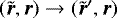 , with
  , and then make m → 0, in order to obtain the Hamiltonian for the motion of the perturbed satellite
![Mathematical equation: \begin{equation*}\begin{split}{\mathcal{H}} \,{=}\, & \frac{\tilde{\bm{r}}\prime^2}{2}-\frac{\mu}{r}+\frac{{\mathcal{G}} m_{0}}{2r_{1}^3}\left[r^2-\frac{3\left(\bm{r}_{1} \cdot\bm{r}\right)^2}{r_{1}^2}\right]-\frac{\mathcal{E}}{r^3}\left[1-3\left(\frac{\bm{r} \cdot\bm{s}}{r}\right)^2\right] \\& -\frac{3\mathcal{E}}{r_{1}^3}\frac{m_{0}}{m_{1}}\left[\frac{\bm{r}_{1} \cdot\bm{r}}{r_{1}^2}-5\frac{\left(\bm{r}_{1} \cdot\bm{r}\right)\left(\bm{r}_{1} \cdot\bm{s}\right)^2}{r_{1}^4}+2\frac{\left(\bm{r}_{1} \cdot\bm{s}\right)\left(\bm{r} \cdot\bm{s}\right)}{r_{1}^2}\right].\end{split}\end{equation*}](/articles/aa/full_html/2022/01/aa41213-21/aa41213-21-eq12.png) (4)
(4)
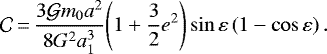
Finally, we average the orbit of the satellite over the mean anomaly (for details see Boué & Laskar 2006), and obtain the secular Hamiltonian
![Mathematical equation: \begin{equation*}\begin{split}{\mathcal{H}}_{\textrm{s}} \,{=}\, & \frac{3{\mathcal{G}} m_{0} a^2}{2r_{1}^3}\left[\bm{e}^2+\frac{1}{2}\frac{\left(\bm{r}_{1} \cdot\bm{u}\right)^2}{r_{1}^2}-\frac{5}{2}\frac{\left(\bm{r}_{1} \cdot\bm{e}\right)^2}{r_{1}^2}\right] \\& +\frac{\mathcal{E}}{2a^3 \Vert{\bm{u}}\Vert^5} \left[\bm{u}^2-3\left(\bm{s} \cdot \bm{u}\right)^2\right]\\&+ \frac{9 a \mathcal{E}}{r_{1}^3}\frac{m_{0}}{m_{1}}\left[\frac{\bm{r}_{1} \cdot\bm{e}}{2 r_{1}^2}\left(1-5\frac{\left(\bm{r}_{1} \cdot\bm{s}\right)^2}{r_{1}^2}\right)+\frac{\left(\bm{r}_{1} \cdot\bm{s}\right)\left(\bm{e} \cdot \bm{s}\right)}{r_{1}^2}\right],\end{split}\end{equation*}](/articles/aa/full_html/2022/01/aa41213-21/aa41213-21-eq13.png) (5)
(5)
with
 (6)
(6)
where k = G∕G is the normal to the orbit of the satellite, i is the unit vector indicating the direction of its pericenter, G is the orbital angular momentum,  , and
, and  . The first term of
  (Eq. (5)) corresponds to the perturbations from the central star, the second term corresponds to perturbations from the gravitational flattening of the planet, while the third term describes the effect of the couple exerted by the central star on the rigid planet on the orbital motion of the satellite.
2.2 Equations of motion
The equations of motion for the vectors e and u can be obtained from the secular Hamiltonian  (Eq. (5)) as (Tremaine et al. 2009; Farago & Laskar 2010)
![Mathematical equation: \begin{equation*}\begin{cases}\frac{\textrm{d} \bm{e}}{\textrm{d}t} \,{=}\,\frac{1}{L}\left(\nabla_{\bm{u}} {\mathcal{H}}_{\textrm{s}} \times\bm{e}+\nabla_{\bm{e}} {\mathcal{H}}_{\textrm{s}} \times\bm{u}\right), \\[6pt]\frac{\textrm{d} \bm{u}}{\textrm{d}t} \,{=}\,\frac{1}{L}\left(\nabla_{\bm{u}} {\mathcal{H}}_{\textrm{s}} \times\bm{u}+\nabla_{\bm{e}} {\mathcal{H}}_{\textrm{s}} \times\bm{e}\right),\end{cases}\end{equation*}](/articles/aa/full_html/2022/01/aa41213-21/aa41213-21-eq19.png) (7)
(7)
which gives
![Mathematical equation: \begin{equation*}\begin{cases}\frac{\textrm{d} \bm{e}}{\textrm{d}t} \,{=}\,\bm{h}_1\times\bm{e}+\bm{h}_2\times\bm{u}+\gamma \, \bm{u}\times\bm{e}, \\[6pt]\frac{\textrm{d} \bm{u}}{\textrm{d}t} \,{=}\,\bm{h}_1\times\bm{u}+\bm{h}_2\times\bm{e},\end{cases}\end{equation*}](/articles/aa/full_html/2022/01/aa41213-21/aa41213-21-eq20.png) (8)
(8)
with
![Mathematical equation: \begin{equation*}\begin{split}\bm{h}_1\,{=}\, &\frac{1}{L}\left[\frac{3{\mathcal{G}} m_{0} a^2}{2r_{1}^5}\left(\bm{r}_{1} \cdot\bm{u}\right)\bm{r}_{1} -\frac{3\mathcal{E}}{a^3\Vert{\bm{u}}\Vert^5}\left(\bm{s}\cdot\bm{u}\right)\bm{\bm{s}}\right], \nonumber\end{split}\end{equation*}](/articles/aa/full_html/2022/01/aa41213-21/aa41213-21-eq21.png)
![Mathematical equation: \begin{equation*}\begin{split}\bm{h}_2\,{=}\, & \frac{1}{L}\left[-\frac{15{\mathcal{G}} m_{0} a^2}{2r_{1}^5}\left(\bm{r}_{1} \cdot\bm{e}\right)\bm{r}_{1} \right. \\&\left. +\frac{9\mathcal{E} am_{0}}{r_{1}^5 m_{1}}\left(\frac{\bm{r}_{1}}{2}-\frac{5}{2}\frac{\left(\bm{r}_{1} \cdot\bm{s}\right)^2}{r_{1}^2}\bm{\bm{r}_{1}} + \left(\bm{r}_{1} \cdot\bm{s}\right)\bm{s} \right) \right],\nonumber\end{split}\end{equation*}](/articles/aa/full_html/2022/01/aa41213-21/aa41213-21-eq22.png)
![Mathematical equation: \begin{equation*}\gamma\,{=}\,{-}\frac{1}{L}\left[\frac{3\mathcal{E}}{2a^3\Vert{\bm{u}}\Vert^5}\left(1-5 \left(\bm{s}\cdot\bm{k}\right)^2\right)+\frac{3{\mathcal{G}} m_{0} a^2}{r_{1}^3}\right]. \nonumber\end{equation*}](/articles/aa/full_html/2022/01/aa41213-21/aa41213-21-eq23.png)
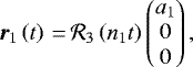
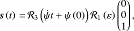
We use Eq. (8) to obtain numerically the secular orbital evolution of the satellite. To completely solve these equations, we also need to compute the motion of the planet around the star, r1 (t), and the evolution of the spin axis, s(t). For simplicity, we assume that the planet moves on a circular orbit and that most of the angular momentum is on its orbit. We also assume that the spin of the planet can only precess around the normal to the ecliptic with constant speed and obliquity (i.e., the angle between the equator of the planet and the ecliptic). Therefore, we have
 (9)
(9)
and
 (10)
(10)
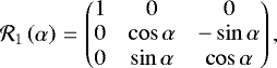
where n1 is the mean motion, ε is the obliquity, and ψ is the precession angle, which measures the precession of the equator with respect to the ecliptic (Fig. 2).  and
and  are the rotations about the x-axis and z-axis, respectively
 (11)
(11)
 (12)
(12)
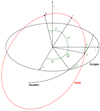 |
Fig. 2 Orbital elements of the orbit of the satellite (in red). |
3 Secular resonances
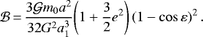
In general, the last term of the secular Hamiltonian (Eq. (5)) is much weaker than the other two terms. For instance, in the case of the Martian satellite Phobos, the ratio between the amplitudes of the third and first term is ~ 10−9. Moreover, on average, the effect of this third term is null over a satellite pericenter precession period. Therefore, we can often neglect its contribution, and the secular Hamiltonian (Eq. (5)) is rewritten as
![Mathematical equation: \begin{equation*}\begin{split}{\mathcal{H}}\,{=}\, & \frac{3{\mathcal{G}} m_{0} a^2}{2a_{1}^3}\left[{e}^2+\frac{1-{e}^2}{2}\left({\bm{\hat r}_{1}} \cdot\bm{k}\right)^2-\frac{5{e}^2}{2}\left({\bm{\hat r}_{1}} \cdot\bm{i}\right)^2\right] \\& +\frac{\mathcal{E}}{2a^3 \left(1-{e}^2\right)^{3/2}} \left[1-3\left(\bm{s} \cdot \bm{k}\right)^2\right],\end{split}\end{equation*}](/articles/aa/full_html/2022/01/aa41213-21/aa41213-21-eq30.png) (13)
(13)
with  . Resonances between the orbit of the satellite and the Sun can only occur due to the first term. In order to identify all possible resonances, we need to develop
  in trigonometric series. This development is given by Yokoyama (2002) but with some misprints. A corrected version is presented in Carvalho & Vilhena de Moraes (2020).
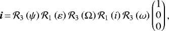
We consider here the ecliptic as reference plane (Fig. 2). Assuming that the satellite is a massless particle and that the orbital angular momentum of the planet is much larger than its rotational angular momentum, the ecliptic remains an inertial plane to a very good approximation. We then need to express  and
and  as a function of the orbital elements of the satellite. The unit vectors k, i and
  can be expressed with respect to the ecliptic as a succession of rotations
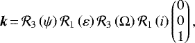 (14)
(14)
 (15)
(15)
and
 (16)
(16)
where λ1 = n1t is the mean longitude of the planet (we assume a circular orbit). The Hamiltonian (Eq. (13)) then becomes
![Mathematical equation: \begin{eqnarray*}{\mathcal{H}}&=&\frac{\mathcal{E}}{2a^3 \left(1-{e}^2\right)^{3/2}} \left[1-3\cos^2 i\right]+\frac{3{\mathcal{G}} m_{0} a^2}{2a_{1}^3}\left[-\frac{{e}^2}{4}\right. \nonumber \\&& \nonumber +\frac{1}{4}{\left(1+\frac{3}{2} {e}^2\right)}\left(\sin^2i+\sin^2{\varepsilon}-\frac{3}{2}\sin^2i\sin^2{\varepsilon}\right)\\&& \nonumber -\frac{1}{8}{\left(1+\frac{3}{2} {e}^2\right)}\sin^2 i\sin^2{\varepsilon}\cos\left(2\Omega\right) \\&& \nonumber +\frac{1}{8}{\left(1+\frac{3}{2} {e}^2\right)}\sin\left(2i\right)\sin\left(2{\varepsilon}\right)\cos\left(\Omega\right)\\&& \nonumber -\frac{5}{8}{e}^2\sin^2i\left(1-\frac{3}{2}\sin^2{\varepsilon}\right)\cos\left(2\omega\right)\\&& \nonumber -\frac{5}{32}{e}^2 \left(1+\cos i\right)^2\sin^2{\varepsilon}\cos\left(2\left(\Omega+\omega\right)\right)\\&& \nonumber -\frac{5}{32}{e}^2 \left(1-\cos i\right)^2\sin^2{\varepsilon}\cos\left(2\left(\Omega-\omega\right)\right)\\&& \nonumber -\frac{5}{16}{e}^2\sin i\left(1+\cos i\right)\sin\left(2{\varepsilon}\right)\cos\left(\Omega+2\omega\right)\\&& \nonumber +\frac{5}{16}{e}^2\sin i\left(1-\cos i\right)\sin\left(2{\varepsilon}\right)\cos\left(\Omega-2\omega\right)\\&& \nonumber -\frac{1}{4}{\left(1+\frac{3}{2} {e}^2\right)}\left(1-\frac{3}{2}\sin^2 i\right)\sin^2{\varepsilon}\cos\left(2\left({\lambda_{1}-\psi}\right)\right)\\&& \nonumber -\frac{1}{16}{\left(1+\frac{3}{2} {e}^2\right)}\sin^2 i\left(1-\cos {\varepsilon}\right)^2\cos\left(2\left({\lambda_{1}-\psi}+\Omega\right)\right)\\&& \nonumber -\frac{1}{16}{\left(1+\frac{3}{2} {e}^2\right)}\sin^2 i\left(1+\cos {\varepsilon}\right)^2\cos\left(2\left({\lambda_{1}-\psi}-\Omega\right)\right)\\&& \nonumber +\frac{1}{8}{\left(1+\frac{3}{2} {e}^2\right)}\sin\left(2i\right)\sin{\varepsilon}\left(1-\cos{\varepsilon}\right)\cos\left(2\left({\lambda_{1}-\psi}\right)+\Omega\right)\\&& \nonumber -\frac{1}{8}{\left(1+\frac{3}{2} {e}^2\right)}\sin\left(2i\right)\sin{\varepsilon}\left(1+\cos{\varepsilon}\right)\cos\left(2\left({\lambda_{1}-\psi}\right)-\Omega\right)\\&& \nonumber -\frac{15}{32}{e}^2\sin^2i\sin^2{\varepsilon}\cos\left(2\left({\lambda_{1}-\psi}+\omega\right)\right)\\&& \nonumber -\frac{15}{32}{e}^2\sin^2i\sin^2{\varepsilon}\cos\left(2\left({\lambda_{1}-\psi}-\omega\right)\right)\end{eqnarray*}](/articles/aa/full_html/2022/01/aa41213-21/aa41213-21-eq39.png)
![Mathematical equation: \begin{eqnarray*}&& \nonumber -\frac{5}{64}{e}^2\left(1+\cos i\right)^2\left(1-\cos{\varepsilon}\right)^2\cos\left(2\left({\lambda_{1}-\psi}+\Omega+\omega\right)\right)\\&& \nonumber -\frac{5}{64}{e}^2\left(1-\cos i\right)^2\left(1-\cos{\varepsilon}\right)^2\cos\left(2\left({\lambda_{1}-\psi}+\Omega-\omega\right)\right)\\&& \nonumber -\frac{5}{64}{e}^2\left(1-\cos i\right)^2\left(1+\cos{\varepsilon}\right)^2\cos\left(2\left({\lambda_{1}-\psi}-\Omega+\omega\right)\right)\\&& \nonumber -\frac{5}{64}{e}^2\left(1+\cos i\right)^2\left(1+\cos{\varepsilon}\right)^2\cos\left(2\left({\lambda_{1}-\psi}-\Omega-\omega\right)\right)\\&& \nonumber -\frac{5}{16}{e}^2\sin i\left(1+\cos i\right)\sin{\varepsilon}\left(1-\cos{\varepsilon}\right)\\&& \nonumber \cos\left(2\left({\lambda_{1}-\psi}\right)+\Omega+2\omega\right)\\&& \nonumber +\frac{5}{16}{e}^2\sin i\left(1-\cos i\right)\sin{\varepsilon}\left(1-\cos{\varepsilon}\right)\\&& \nonumber \cos\left(2\left({\lambda_{1}-\psi}\right)+\Omega-2\omega\right)\\&& \nonumber -\frac{5}{16}{e}^2\sin i\left(1-\cos i\right)\sin{\varepsilon}\left(1+\cos{\varepsilon}\right)\\&& \nonumber \cos\left(2\left({\lambda_{1}-\psi}\right)-\Omega+2\omega\right)\\&& \nonumber +\frac{5}{16}{e}^2\sin i\left(1+\cos i\right)\sin{\varepsilon}\left(1+\cos{\varepsilon}\right)\\&&\left.\cos\left(2\left({\lambda_{1}-\psi}\right)-\Omega-2\omega\right)\right].\end{eqnarray*}](/articles/aa/full_html/2022/01/aa41213-21/aa41213-21-eq40.png) (17)
(17)
From this Hamiltonian, we can identify 14 different possible combinations of angles between the orbital motion of the planet and the secular motion of the satellite. The corresponding possible resonances are then
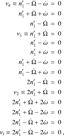 (18)
(18)
where  is the mean motion of the planet corrected by the precession frequency of the spin axis.
The argument of the pericenter, ω, is not an inertial angle, as it is defined with respect to the line of nodes between the orbit of the satellite and the equator of the planet (Fig. 2), but it can be related with the inertial longitudes ω = ϖ − Ω. The first resonance in the list (18) thus becomes  , and occurs when the pericenter precession frequency of the satellite,
  , is equal to
  . This corresponds to the well-known evection resonance. When capture in this resonance occurs, we can observe a significant increase in the eccentricity of the satellite (e.g., Touma & Wisdom 1998; Frouard et al. 2010). However, the amplitude of the evection resonance is proportional to e2, and so this resonance cannot occur for satellites in nearly circular orbits, which is the final outcome of tidal evolution. The resonance
  has been studied in the case of Phobos by Yoder (1982), who showed that its crossing could lead to a sudden increase in the eccentricity of Phobos of maximal amplitude 0.016. We also note that in expression (17) other secular resonances not involving the mean motion n1 are also possible, such as
  (Kozai resonance), but we do not study them here.
4 Eviction-like resonances
The last resonance in the list (18),  , corresponds to the “eviction” resonance described by Touma & Wisdom (1998), who showed that it can increase the inclination of the satellite. In principle, any resonance containing the longitude of the ascending node, Ω, can excite the inclination, and hence be dubbed as “eviction-like” resonance. However, as for the evection resonance, the amplitudes of most of these resonances are also proportional to the square of the eccentricity (Eq. (17)), and so they are not present for nearly circular satellite orbits. This incidentally includes the “original” eviction resonance νi reported by Touma & Wisdom (1998).
In the Hamiltonian (17), only four resonances,  and
and  , do not depend on the pericenter precession frequency, and thus do not have a null amplitude for an eccentricity equal to zero. As a consequence, they are able to modify the inclination of a satellite even if the eccentricity is nearly zero, as currently observed for all tidally evolved satellites in the solar system. Nonetheless, since n1 > 0 and
  is expected to be negative for a prograde orbit, only the resonances
  and
and  can occur (Yokoyama 2002). Therefore, in this section, we focus our study on these two resonances.
In general, we have  , thus, for simplicity, we assume
  only in this section, such that we can use the Delaunay canonical variables. It is possible to obtain these variables for a moving equator, butwe needed to modify the Hamiltonian (e.g., Goldreich 1965; Kinoshita 1993).
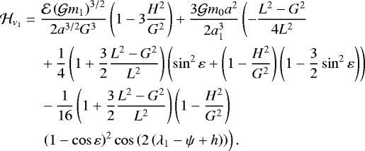
4.1 Resonance ν1
We denote ν1 the resonance associated to the relation  . Among the resonant terms of the Hamiltonian (17), we keep only the term associated with ν1, and we get for the resonant Hamiltonian
![Mathematical equation: \begin{equation*}\begin{split}\mathcal{H}_{\nu_1}\,{=}\,&\frac{\mathcal{E}}{2a^3 \left(1-{e}^2\right)^{3/2}}\left(1-3\cos^2 i\right) + \frac{3{\mathcal{G}} m_{0} a^2}{2a_{1}^3}\left(-\frac{{e}^2}{4}\right. \\[3pt]& +\frac{1}{4}{\left(1+\frac{3}{2} {e}^2\right)}\left(\sin^2i+\sin^2{\varepsilon}-\frac{3}{2}\sin^2i\sin^2{\varepsilon}\right)\\[3pt]& \left.-\frac{1}{16}{\left(1+\frac{3}{2} {e}^2\right)}\sin^2 i\left(1-\cos {\varepsilon}\right)^2\cos\left(2\left({\lambda_{1}-\psi}+\Omega\right)\right)\right).\end{split}\end{equation*}](/articles/aa/full_html/2022/01/aa41213-21/aa41213-21-eq57.png) (19)
(19)
Using the Delaunay variables for the satellite (L, G, H, l, g, h), where  ,
,  , H = Gcosi, l = M, g = ω, and h = Ω, we obtain
 (20)
(20)
The Hamiltonian  does not depend on the angles l and g, and so the associated action variables L and G are constant. As a result, the semi-major axis and the eccentricity are also constant, that is, the ν1 resonance does not modify the eccentricity. By removing the constant terms and the terms which do not depend on H or h, the Hamiltonian becomes
 (21)
(21)
with
 (22)
(22)
 (23)
(23)
As in Touma & Wisdom (1998) and Yokoyama (2002), we use a generating function to perform a canonical change of variables, F1 = (λ1 − ψ + h)X. We obtain the canonical variables (X, x) with X = H and x = λ1 − ψ + h. As we suppose  in this section, we have ∂(λ1 − ψ)∕∂t = n1, and the Hamiltonian becomes
 (24)
(24)
The equations of motion are then given by
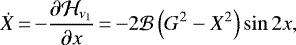 (25)
(25)
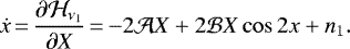 (26)
(26)
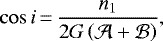
This Hamiltonian possesses four fixed points, obtained when (Ẋ, ẋ) = (0, 0): the point  and the point
  are stable, while the points
  and
and  are unstable. In Fig. 3, we show the level curves of the Hamiltonian (24) for Phobos, assuming an obliquity ε = 90° for Mars (Table 1), where we can clearly identify the fixed points as well as the separatrix that encircles the resonant area. If the satellite is at a stable fixed point, its inclination verifies
 (27)
(27)
while for an unstable fixed point, the inclination is given by
 (28)
(28)
Therefore, the stable points are present only if  , and the unstable ones if
  . The two equilibrium points are usually very close to each other. Indeed, near the ν1 resonance, the perturbation due to the flattening of the planet is in general much larger than the stellar perturbation, and so
 (29)
(29)
In Fig. 4, we show the stable equilibria for Phobos computed with the values from Table 1, assuming an obliquity of Mars similar to the present one, ε = 25°. We observe that there is a critical value for the semi-major axis of the satellite (obtained with cos i = 1),
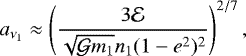 (30)
(30)
above which the ν1 resonance is not present. In the case of Phobos, we have 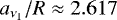 . This value is very close to the surface of Mars, but still larger than the Roche limit for a solid body with the density of Phobos, a∕R≈ 1.61 (e.g., Chandrasekhar 1987).
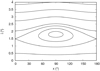 |
Fig. 3 Level curves of the Hamiltonian (24) for Phobos (Table 1), for a semi-major axis a = 2.61686 R, and assuming an obliquity ε = 90° for Mars. |
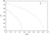 |
Fig. 4 Evolution of the inclination of Phobos for the stable fixed points with respect to its semi-major axis for the ν1 resonance (red curve) computed with Eq. (27), and for the ν2 resonance(blue curve) computed with Eq. (37) for a Martian obliquity of ε = 25°. The Roche limit for Phobos is a∕R ≈ 1.6. |
Values of the present parameters of Phobos, Mars, and the Sun used in this work.
4.2 Resonance ν2
We denote ν2 the resonance associated to the relation  . Among the resonant terms of the Hamiltonian (17), we keep only the term associated with ν2, and we get for the resonant Hamiltonian
 (31)
(31)
As for the ν1 resonance, the Hamiltonian does not depend on the angle g and the eccentricity remains constant. The Hamiltonian then becomes
 (32)
(32)
where  is given by expression (22), and
 (33)
(33)
We now consider the generating function F2 = (2(λ1 − ψ) + h)Y. The canonical variables (Y, y) verify Y = H and y = 2(λ1 − ψ) + h, and the resonant Hamiltonian becomes
 (34)
(34)
The equations of motion are then given by
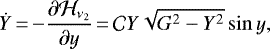 (35)
(35)
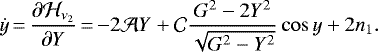 (36)
(36)
The fixed points are then located at y = 0 or y = π. In order to obtain the Y values for the fixed points, we must solve the following quartic equation
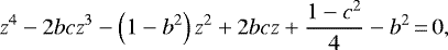 (37)
(37)
with z = Y∕G,  , and
, and  . Contrary to the ν1 resonance, it is not possible to find a simple analytical expression for the fixed points, although we can find theroots numerically. In Fig. 4, we show the stable fixed point located at y = π for Phobos with the values from Table 1, and assuming an obliquity of Mars similar to the present one, ε = 25°. For a satellite close to the ν2 resonance, the perturbations due to the flattening of the planet are in general larger than the stellar perturbations, and so
  . It is then possible to obtain an approximate value for the inclination of the fixed points. By neglecting the term proportional to
  in Eq. (36), we obtain
 (38)
(38)
and the inclination is given by
 (39)
(39)
Therefore, as for the ν1 resonance, there is a critical value  of the semi-major axis above which the ν2 resonance is not present. An approximate value of
  is given by (obtained with cosi = 1)
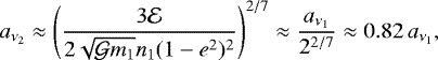 (40)
(40)
where  is the critical value for the ν1 resonance (Eq. (30)). In the case of Phobos, we have
  .
.
4.3 Capture probabilities
Due to tidal effects, the semi-major axis of the satellites usually evolves with time. When the semi-major axis is increasing, the eviction-like resonances are crossed if we initially have a < aν. As a result,capture is not possible, because the resonances are no longer present for a > aν (Fig. 4). As noted by Touma & Wisdom (1998), the crossing of the resonance can nevertheless lead to a sudden variation in the inclination of the satellite due to the conservation of the area in the phase plane (Fig. 3).
On the other hand, when the semi-major axis is decreasing, the eviction-like resonances are encountered if we initially have a > aν. As a result, capture in resonance may occur. In that case, as the semi-major axis is decreasing, the inclination increases (Fig. 4). We then conclude that, for a satellite with an orbit close to the equator, capture in eviction-like resonances is only possible if the semi-major axis is decreasing.
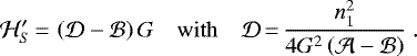
It is possible to compute analytically the capture probability in the ν1 resonance, provided that the evolution of the semi-major axis is adiabatic. To be considered as adiabatic, the evolution of the semi-major axis must be much slower than the conservative inclination variations, that is, tidal dissipation must be weak. In general, in the phase space of a given resonance we can distinguish three different regions delimited by the separatrix of the resonance (Fig. 3): a libration zone, with area Alib, and two circulation zones, one above the libration zone, with area Acirc, and another below the libration zone, with area  . The capture probability is then obtained by the modification of the phase space with time, that is, by the change in the areas encircled by the separatrix (Yoder 1979; Henrard 1982, 1993)
 (41)
(41)
where Atot corresponds to the sum of the libration area with the circulation area increasing with time. The ordinate of the stable fixed point inside the libration area is (Eq. (27))
 (42)
(42)
and so the ordinate of the fixed point decreases when the semi-major decreases, which means that the circulation area whose surface increases with time is Acirc, and then Atot = Alib + Acirc.
As the phase space of the ν1 resonance is π−periodic (Eq. (24)), we restrict the computation of the capture probabilities to x ∈ [0 : π]. We perform the following canonical change of variables (X, x) → (z, x) with z = X∕G = cosi. With these variables, the Hamiltonian (24) becomes
 (43)
(43)
To compute the libration area, we need to know the equation of the separatrix. The unstable fixed point (28) is on the separatrix, whose energy is
 (44)
(44)
The equation of the separatrix is then
 (45)
(45)
and so, the equations of the superior separatrix, z+, and the inferior one, z−, are
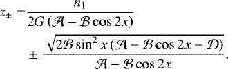 (46)
(46)
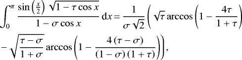
The libration area encircled by the separatrix is
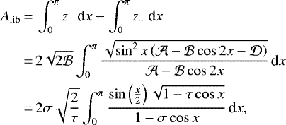 (47)
(47)
with
 (48)
(48)
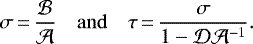
In order that the separatrix and the libration area exist, we must have  . Therefore, σ and τ verify 0 < σ < τ < 1. We obtain
 (49)
(49)
and finally
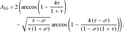 (50)
(50)
For the total area we get
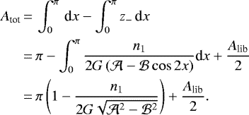 (51)
(51)
If we consider only the tidal effects on the semi-major axis, in the expressions of Alib and Atot only the semi-major axis depends on the time. Then, from expression (41) the capture probability is given by
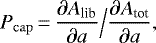 (52)
(52)
which does not depend on the dissipation law chosen for the semi-major axis. From the expressions of Alib (Eq. (50)), and ofAtot (Eq. (51)), we can compute the derivatives with respect to the semi-major axis, and finally the capture probability.
In Fig. 5, we show the capture probability in the ν1 resonance for Phobos as a function of the obliquity of Mars (with initial values taken from Table 1). The solid line gives the theoretical estimation obtained with expression (52), using a critical semi-major axis obtained with expression (27). In order to obtain a numerical estimation of the capture probability with different values of the tidal dissipation (for more details see Eq. (56) and Sect. 6.2), we perform numerical integrations of the resonant Hamiltonian (19). We modify this Hamiltonian following Goldreich (1965) and Kinoshita (1993) to consider the motion of the Martian equator, which we model here with a constant obliquity and a uniform precession.
For the present tidal dissipation of Mars (Q = 99.5), there are some differences between the numerical results and the analytic computation. However, for weaker tidal dissipation (Q = 5000), which corresponds to a slower evolution of the semi-major axis of Phobos (adiabatic evolution), we observe that there is a good agreement. We hence conclude that the evolution of Phobos cannot be considered as adiabatic.
In Fig. 6, we show the theoretical capture probability (Eq. (52)) also as function of the obliquity of Mars, but for different inclinations and eccentricities of Phobos. As expected, we observe that the capture probability increases with the obliquity, because for small obliquity, ε, the amplitude of the ν1 resonance is proportional to ε4 (Eq. (19)). On the other hand, we observe that the capture probability strongly decreases with the inclination of Phobos. The red curve, obtained with e = 0, is very close to the black curve, obtained with e = 0.015, that is, the capture probability is not much influenced by a small variation in eccentricity. This was also expected, since the amplitude of the ν1 resonance is proportionalto 1 + 3e2∕2 (Eq. (19)).
The Hamiltonian of the ν1 resonance is similar to the one of the second order ivection resonance studied by Xu & Fabrycky (2019) in the case of a binary star system. Theresonances called ivection by Xu & Fabrycky (2019) correspond to a resonance between the node precession frequencies of planets orbiting around a star with the mean motion of the binary. At the lowest order in the mutual inclination of planets, Xu & Fabrycky (2019) obtained that the Hamiltonian of the second order ivection resonance can be written in the same dimensionless form as the j + 2 : j orbital resonance described by Borderies & Goldreich (1984). In the limit of small inclination, it is then also possible to use the analytical expression for the capture probability given by Borderies & Goldreich (1984).
The capture probabilities in the ν2 resonance can be obtained with a similar method as for the ν1 resonance. However, unfortunately it is not possible to find a simple analytical expression for the corresponding Alib integral (Eq. (47)). At the lowest order in inclination of the satellite, the ν2 resonance and the first order ivection resonance of Xu & Fabrycky (2019) can be written in the same dimensionless form as the j + 1 : j orbital resonance described by Borderies & Goldreich (1984). In the limit of small inclination, the analytical expression of the capture probability given by Borderies & Goldreich (1984) can then also be used for the ν2 resonance.
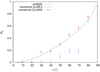 |
Fig. 5 Capture probability of Phobos in the ν1 resonance with respect to the obliquity of Mars. The black curve corresponds to the capture probability computed with Eq. (52). The blue crosses and the red dots correspond to the capture probability determined for each value of the obliquity with N = 720 numericalintegrations of the resonant Hamiltonian (Eq. (19)), respectively with Q = 99.5 and Q = 5000 for the effective specific tidal dissipation. The errorbars are given by |

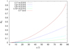 |
Fig. 6 Capture probability of Phobos in the ν1 resonance with respect to the obliquity of Mars for different orbital parameters of Phobos. The black line corresponds to the current parameters. |
5 Interaction between resonances
In previous section, we have studied the dynamics of an isolated resonance. However, in the full Hamiltonian (17) there is a large number of resonant terms that may interact. This is particularly true, when two resonant islands are close to each other, as it is the case of the ν1 resonance and the evection resonance νe (Yokoyama 2002). Indeed, in general we have  , which is thecase for a satellite with a weakly inclined orbit with respect to the equator of its planet. Thus, for nonzero eccentricities, the libration width of these two resonances may overlap and trigger chaotic motion (Chirikov 1979). In order to describe this interaction, we need to add to the previous ν1 resonant Hamiltonian (19) the term corresponding to the evection resonance νe. The interaction Hamiltonian is then
![Mathematical equation: \begin{equation*}\begin{split}\mathcal{H}_{\textrm{int}} = & \frac{\mathcal{E}}{2a^3 \left(1-{e}^2\right)^{3/2}}\left(1-3\cos^2 i\right) + \frac{3{\mathcal{G}} m_{0} a^2}{2a_{1}^3}\left(-\frac{{e}^2}{4}\right. \\[3pt]& +\frac{1}{4}{\left(1+\frac{3}{2} {e}^2\right)}\left(\sin^2i+\sin^2{\varepsilon}-\frac{3}{2}\sin^2i\sin^2{\varepsilon}\right)\\[3pt]& -\frac{1}{16}{\left(1+\frac{3}{2} {e}^2\right)}\sin^2 i\left(1-\cos {\varepsilon}\right)^2\cos\left(2\left({\lambda_{1}-\psi}+\Omega\right)\right)\\[3pt]& \left.-\frac{5}{64}{e}^2\left(1+\cos i\right)^2\left(1+\cos{\varepsilon}\right)^2\cos\left(2\left({\lambda_{1}-\psi}-\varpi\right)\right)\right).\end{split}\end{equation*}](/articles/aa/full_html/2022/01/aa41213-21/aa41213-21-eq115.png) (53)
(53)
5.1 Frequency analysis method
The interaction Hamiltonian has two degrees of freedom, and it is thus not integrable. This kind of problem is often studied using surface sections, but here we propose a different method: we use stability maps based on frequency analysis (Laskar 1988, 1990, 1993, 2003; Laskar et al. 1992). This method decomposes a discrete temporal function in a quasi-periodic approximation and can estimate its stability. We consider a grid of initial conditions and integrate the equations of motion over a time T. Then, we perform a frequency analysis1 over the time intervals [0 : T∕2] and [T∕2 : T], and determine the precession frequency of the ascending node of the satellite in each interval, f1 and f2, respectively. The stability is measured by
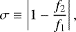 (54)
(54)
which estimates the chaotic diffusion of the precession frequency (Dumas & Laskar 1993; Laskar 1993). The larger σ is, the more unstable the orbital motion of the satellite is. For stable motion we have σ ~ 0, while σ ≪ 1 if the motion is weakly perturbed, and σ ~ 1 when the motion is chaotic. It is difficult to know precisely what is the value of σ for which the motion is stable or unstable, but a threshold of stability σs can be estimated such that most of the trajectories with σ < σs are stable (Couetdic et al. 2010). For σ < σs, we still would like to distinguish the circulation trajectories from those that are in resonance. For that purpose, in those cases we compute a second quantity
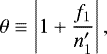 (55)
(55)
which measures the relative difference between the precession frequency and the resonance frequency  . We assume that a trajectory is in resonance when θ < θr, where the boundary θr is chosen such that it is able to correctly identify the libration area in the case of the resonant Hamiltonian (19). In the stability maps, we attribute a color scheme to the different σ going from blue (stable) to red (unstable), while for the resonant trajectories we apply a black filter.
5.2 Stability maps
As for surface sections, the frequency analysis is a numerical method, and thus we need to attribute values to the parameters of the system. We adopt here the values for Phobos and Mars (Table 1) near the ν1 resonance, for which  . This resonance is more interesting than the ν2 resonance, since it is close to the evection resonance νe. We also fix the obliquity of Mars at ε = 90°, because the resonance width of ν1 is larger for this obliquity (Eq. (19)) for ε ∈ [0° : 90°]. We build a 2D mesh of initial conditions where the inclination of the satellite varies from 0.04° to 4° with a step size of 0.04°, and the canonical variable x = λ1 − ψ + Ω varies from 0° to 180° with a step size of 2°, and we integrate the equations of motion over the time interval T = 80 kyr.
In Fig. 7, we show the stability maps obtained for different initial values of the eccentricity of Phobos e = 10−5, 0.015, 0.030,and 0.045, since the amplitude of the evection resonance increases with the eccentricity (Eq. (53)). For each value of the initial eccentricity, we numerically integrate the equations of motion obtained for the full secular Hamiltonian  (Eq. (5)), for the resonant Hamiltonian
 (Eq. (19)), and for the interaction Hamiltonian
  (Eq. (53)). For the three cases, we consider that the Martian obliquity is constant, and that the precession of the Martian equator is uniform. To consider the motion of the Martian equator, we modify the resonant Hamiltonian
  and the interaction Hamiltonian
 following Goldreich (1965) and Kinoshita (1993). That is, we obtain three different maps for each eccentricity value2 : the left-hand map corresponds to the integrable resonant Hamiltonian for the ν1 resonance (Eq. (19)), the middle map corresponds to the sum of this resonant Hamiltonian with the term due to the evection resonance (Eq. (53)), and the right-hand map illustrates the true dynamics of the system obtained with the full secular Hamiltonian (Eq. (5)). The resonant Hamiltonian (Eq. (19)) gives identical trajectories for the initial conditions x and x + π, that is why we only consider x ∈ [0°, 180°]. This symmetry is broken when we introduce the perturbations from the other resonant terms, but the changes are almost imperceptible.
We attribute a color scheme to the different values of σ, and estimate for the stability threshold3, log10σs = −4.4. Therefore, the blue and green areas correspond to stable circulating trajectories, while the yellow, orange, and red ones correspond to chaotic motions. In the panels corresponding to the resonant Hamiltonian (left-hand maps in Fig. 7), we additionally show the level curves of constant energy obtained with expression (19), as this problem is integrable (see also Fig. 3). We observe there is a good agreement between these curves and the stability map obtained with frequency analysis. These panels thus allow us to calibrate the transition between the libration and circulation areas. We find that trajectories inside the separatrix are bounded by log10θr = −3.9 (Eq. (55)). We then apply a black filter for stable trajectories with θ < θr that correspond to resonant regions4.
In Fig. 7, we observe that as we increase the eccentricity, the dynamics changes considerably between the resonant case and the full problem. However, a first striking evidence is that the evection resonance νe is the major responsible for this modification, since the middle maps obtained only with the interaction Hamiltonian (Eq. (53)) are very similar to the right-hand maps obtained with the full secular Hamiltonian (Eq. (5)). This means that the dynamics of Phobos around the ν1 resonance is essentially governed by the interaction between ν1 and νe. More detailed studies of this problem, thus only need to take the two-degree of freedom Hamiltonian (53) into account.
As expected, for a nearly zero eccentricity, e = 10−5 (first row in Fig. 7), all maps are similar to the one obtained with the resonant Hamiltonian (19). Indeed, for such a small eccentricity, the amplitude of the evection resonance νe is nearly zero, and the dynamics is dominated by the ν1 resonance. Nonetheless, in the case of the full Hamiltonian we observe already some diffusion of the orbits in the region around the libration area, because the eccentricity is not exactly zero. For the present eccentricity of Phobos, e = 0.015 (second row in Fig. 7), the ν1 resonance still presents a large libration area in the full Hamiltonian case, but is now surrounded by a large chaotic region. Its chaotic nature is notably characterized by a high fickleness of the value of the diffusion index, σ. For an eccentricity of e = 0.03 (third row in Fig. 7), the libration area corresponding to the ν1 resonance still exists, but it is considerably smaller and deformed, while for e = 0.045 (last row in Fig. 7) the ν1 resonance almost disappeared in the middle of a chaotic region. Finally, we also observe for the full secular Hamiltonian and the resonant Hamiltonian that as the eccentricity increases, the center of the libration area is slightly shifted toward increasing values of x> 90°.
In Fig. 7, we confirm that the interaction between the resonances ν1 and νe increases with the eccentricity. For the present eccentricity of Phobos (or smaller), this interaction is not very important. As a result, in the future Phobos may survive in the ν1 resonance. However, as the eccentricity increases, we observe that the chaotic region around ν1 progressively replaces the libration area. It is thus unlikely for a satellite with eccentricities larger than 0.05 to be captured in this resonance.
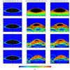 |
Fig. 7 Stability maps for Phobos (Table 1) using an obliquity for Mars ε = 90°. From top to bottom, the initial eccentricity is e = 10−5, e = 0.015, e = 0.03, e = 0.045. Each column corresponds to the integration using different Hamiltonians: resonant Hamiltonian (left), interaction Hamiltonian (middle) and the full secular Hamiltonian (right). The color scale indicates the value of the quantity log10 σ. The blue and green areas correspond to stable circulating trajectories, while the yellow, orange, and red ones correspond to chaotic motions. The black areas correspond to stable resonant regions, for which log10 θ < −3.9. |
6 Application to Phobos
In order to maximize the impact of the eviction-like resonances on the inclination of a satellite, the semi-major axis must decrease. Tidal interactions between the satellite and the planet can account for this evolution, provided that the orbital period of the satellite is shorter than the rotational period of the planet, which is the case of Phobos, the largest satellite of Mars (e.g., Szeto 1983). Among the main satellites of solar system planets, only Triton, the largest satellite of Neptune, is also spiraling into the planet, but because it is on a retrograde orbit (e.g., Correia 2009). Therefore, in this section we apply our model to study Phobos.
At present, the semi-major axis of Phobos is a∕R = 2.761, and the eccentricity is e = 0.01511 (Jacobson & Lainey 2014). Among the fourteen resonances listed in Eq. (18), seven resonances can act on a prograde satellite such as Phobos. During its past evolution, Phobos already encountered four of these resonances, but their effect on its orbit is presumably to have been negligible (Yokoyama 2002), since the amplitudes of these resonances are proportional to the square of the eccentricity. In the future, Phobos will encounter the νe and the ν1 resonances, which occur almost simultaneously around  , and later the ν2 resonance, which is located at
  . For the ν1 and the ν2 resonances, the amplitudes are not null for eccentricities close to zero, and so they can modify the future inclination of Phobos.
In Sect. 4.3, we have obtained the capture probability with an analytical computation. However, expression (52) is only valid for the ν1 resonance and if the evolution is adiabatic. Moreover, it does not take the interaction between the ν1 resonance and the evection resonance νe into account, that we have seen in Sect. 5. It is then necessary to perform numerical simulations to capture the correct dynamics while crossing the ν1 and ν2 resonances. Here we investigate the capture probabilities in these two resonances, and determine which parameters can influence this capture. In the case where capture is not possible, we also study the effects due to the crossing of these resonances on the orbital evolution of Phobos.
6.1 Numerical model
We numerically integrate the set of equations (7) to obtain the secular orbital evolution of Phobos forced by the orbital motion of Mars and its equator. We consider that the orbit of Mars in the ecliptic is circular and that its equator has a uniform precession and a constant obliquity.
Tides raised by Phobos on Mars, modify all the orbital parameters of the satellite with time. However, for simplicity we consider only the evolution of the semi-major axis. We also do not consider tides raised by Mars on Phobos, whose effect is very small, since the rotation of Phobos is currently synchronous and on a near circular orbit. In order to describe the evolution of the semi-major axis, we adopt a constant − Q tidal model (e.g., Szeto 1983),
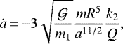 (56)
(56)
where m is the mass of Phobos, R is the radius of Mars, k2 is the second Love number, and Q is the effective specific tidal dissipation. From the observation of the satellites of Mars, it is possible to put constraints on the coefficients k2 and Q. We adopt the values obtained by Jacobson & Lainey (2014) with this method: k2 = 0.183 and Q = 99.5 (Table 1).
6.2 Numerical setup
The capture probability in eviction-like resonances depends on the inclination of the satellite and on the obliquity of the planet (Sect. 4.3). However, it can also depend on the eccentricity, because of the interaction with neighbor resonances (Sect. 5). The current eccentricity of Phobos is about 0.015, but it is still being damped to smaller values. It is then likely that it will be smaller when Phobos approaches the resonances. Then, in order to observe the impact of the eccentricity in the capture probability, we adopt different eccentricity values up to 0.015.
The obliquity of Mars is chaotic and cannot be precisely computed beyond about 10 Myr (Touma & Wisdom 1993; Laskar & Robutel 1993; Laskar et al. 2004). It experiences variations between 0° and 60° over 50 Myr, and can even reach values beyond 60° over higher periods of time. For instance, over 100 Myr, the obliquity has a probability of 7.23% to reach 60° and cannot have values beyond 70°, but over 5 Gyr, the probabilities for the obliquity to reach 60°, 70°, and 80°, are respectively 95.35%, 8.51%, and 0.015% (Laskar et al. 2004). Due to the decrease in the semi-major axis, it is expected that Phobos will collide with Mars in about 40 Myr (Efroimsky & Lainey 2007). It is then very unlikely that Mars has an obliquity higher than 60° when Phobos encounters the eviction-like resonances. We nevertheless investigate the probability of capture for all obliquity values up to 90°, in order to get a global vision of this mechanism.
To numerically estimate the capture probability in resonance, for each initial value of the eccentricity and obliquity we perform 720 simulations varying the initial longitude of the ascending node Ω from 0° to 359.5° with a step of 0.5°, while fixing the remaining initial parameters.
The rotational and orbital motion of Mars is complex, but can be approximated with quasi-periodic solutions (e.g., Ward 1979; Laskar 1990; Laskar & Robutel 1993; Laskar et al. 2004). In such solutions, the Martian obliquity is not constant, but the current dominant term corresponds to rapid oscillations, which can induce variations between 10.8° and 38.0° with a period of about 120 kyr (Ward 1979). Therefore, its evolution time-scale is much longer than the precession motion of Phobos, and so it can be considered constant during the resonance crossing. We consider a fixed orbit for Mars and a uniform precession of the Martian equator, that is, without taking the planetary perturbations into account that induce secular variations in periods much longerthan the precession motion of Phobos. We also consider a circular orbit for Mars to simplify the problem.
6.3 Resonance ν1
6.3.1 Capture probabilities
We compute the capture probabilities in the ν1 resonance using the present inclination of Phobos, i = 1°. For the eccentricity, we adopt values e = 0, 10−5, 10−4, 10−3 and 0.015, while for the obliquity we adopt values from 0° to 60° with a step of 10°, and from 60° to 90° with a step of 2°, since the variations in the capture probability are more important when the obliquity is high (Sect. 4.3). We start our simulations for a semi-major axis slightly larger than  (Eq. (30)) and integrate the equations of motion for 500 kyr. The results are shown in Fig. 8.
As expected, we observe that the capture probability in the ν1 resonance increases with the obliquity (Sect. 4.3). For all the considered eccentricities, we did not observe any capture for an obliquity smaller than 60°, and when ε = 60°, a unique capture occurred (for e = 10−4). The probability of capture for e = 0 increases from 0.28% for ε = 66° to 81.4% for ε = 90°. For an initial eccentricity of 0.015, which corresponds to the current value of the eccentricity, the probability of capture is zero except for ε = 82° and ε = 90°, where one and two captures have been observed, which correspond to capture probabilities of about 0.14% and 0.28%, respectively. These results are consistent with those observed by Yokoyama (2002), but present some disagreement with the theoretical estimations done in Sect. 4.3. One reason is because tides acting on Phobos semi-major axis are very strong (Eq. (56)), and hence the evolution is not adiabatic (see Fig. 5). The other reason is the perturbations from the evection resonance (Sect. 5).
According to expression (19), the influence of the eccentricity should be weak, because the resonance width slightly increases with the eccentricity. However, in Fig. 8, we note that the probability of capture sharply decreases when the eccentricity slightly increases. For instance, for an obliquity of 90°, the probability is 81.4% for e = 0, 61.7% for e = 10−5, 19.2% for e = 10−4, and 3.6% for e = 10−3. This is somehow surprising, because in Fig. 7 we observe that for the present eccentricity (e = 0.015) a large resonance island is still present. However, as seen in previous sections, the ν1 resonance is very close to the evection resonance νe. As the semi-major axis of Phobos is decreasing, this resonance occurs almost simultaneously with the ν1 resonance. Capture in the evection resonance is not possible, but crossing it induces a variation in the eccentricity of Phobos as we can see in Figs. 9–11.
In Fig. 12, we plot the maximum and minimum differences, Δe, between the mean eccentricity before and after the encounter with the ν1 resonance asa function of the obliquity, when the capture succeeds and fails. If the capture fails, regardless of the initial value of the eccentricity before encountering the ν1 resonance, the final mean eccentricity always increases. We note that during the crossing of the ν1 resonance the eccentricity can even take higher values before decreasing to a smaller final value (Figs. 10 and 11). For small obliquities, the eccentricity is always strongly excited by about 0.04 (e.g., for ε = 0°, we have 0.0365 < Δe < 0.0395), which is consistent with the results previously observed by Yoder (1982) and Yokoyama (2002). For obliquities larger than 60°, we observe a smaller average variation around 0.02, that can nevertheless still temporarily increase to about 0.04 (e.g., for ε = 90°, we have 0.005 < Δe < 0.0298). For these larger eccentricity values, the libration width of the ν1 resonance ismuch smaller and the capture probability is hence considerably reduced (see Fig. 7).
In Fig. 12, we also show the statistics when capture succeeds5. In this case,we observe smaller variations in the eccentricity. Therefore, the chances of capture in the ν1 resonance are weak because of the nearby evection resonance νe. This resonance leads to an increase in the eccentricity, which in turn gives rise to a chaotic region around the ν1 resonance that reduces its libration width (see Sect. 5).
We conclude that capture in the ν1 resonance can only occur for very small eccentricity values and for an obliquity higher than 60°. These chances are on the low side, because as we have just seen, the eccentricity of Phobos will likely increase after crossing the evection resonance, and the obliquity of Mars is not expected to exceed 60° in the next 40 Myr. It is then extremely unlikely that in the future Phobos gets caught in the ν1 resonance. Nevertheless, if ever capture occurs, this resonance is stable and the inclination can increase. Indeed, in Fig. 9 we show an example of this capture and subsequent evolution for e = 0.015 and ε = 90°. We also confirmthat, when capture occurs, the inclination follows the equilibrium point given by expression (27).
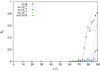 |
Fig. 8 Capture probabilities of Phobos in the ν1 resonance with respect to the obliquity of the equator of Mars for different initial eccentricities. |
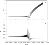 |
Fig. 9 Evolution of the inclination (a) and of the eccentricity (b) during the capture in the ν1 resonance for an obliquity of ε = 90° with the initial conditions e = 0.015 and Ω = 351.5°. The blue curve corresponds to the stable fixed point of the ν1 resonance computed with Eq. (27). |
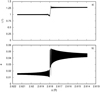 |
Fig. 10 Evolution of the inclination (a) and of the eccentricity (b) during the crossing of the ν1 resonance for an obliquity of ε = 60° with the initial conditions e = 0.015, and Ω = 231°. |
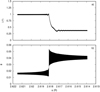 |
Fig. 11 Evolution of the inclination (a) and of the eccentricity (b) during the crossing of the ν1 resonance for an obliquity of ε = 60° with the initial conditions e = 0.015, and Ω = 203°. |
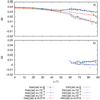 |
Fig. 12 Evolution of the maximum and minimum variations in the mean eccentricity Δe owing to the encounter with the ν1 resonance in the cases where the capture in the resonance fails (a), and succeeds(b), with respectto the obliquity for different initial eccentricities. |
6.3.2 Inclination variation
When capture in resonance does not occur, we still observe inclination variations during the resonance crossing. As for the capture probability, the exact behavior of the inclination depends on the initial value of the longitude of the ascending node. In Figs. 10 and 11, we show two examples of such variations in the case of the ν1 resonance, which correspond to an increase and to a decrease in the initial inclination, respectively. These variations modify the state of a satellite and can lead to misinterpretations of its origin. We can profit from the simulations already performed to estimate the capture probabilities to put limits on the inclination variations. Moreover, the ν2 resonance is encountered after the ν1 resonance, and so it is important to estimate the inclination of Phobos after crossing the ν1 resonance, because the capture probability depends on the inclination (Sect. 4.3).
In Fig. 13, we show the maximum and minimum differences between the mean inclination of Phobos before and after the crossing of the ν1 resonance. As for the capture probability, we observe that these variations depend on the initial eccentricity and obliquity. The variations increase in general with the obliquity: they are nearly zero for obliquities below 40°, but they can present an amplitude variation of about 1° for obliquities larger than 60°. This can seem a modest variation, but given that the present inclination of Phobos is also 1°, it corresponds to a change around 100%. If the eccentricity of Mars is considered, Yokoyama et al. (2005) observe that, for some initial conditions, the eccentricity and the inclination after the crossing of the resonance can even increase to about 0.08 and 4°, respectively.
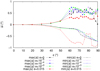 |
Fig. 13 Evolution of the maximum and minimum variations in the mean inclination Δi owing to the encounter with the ν1 resonance in the case where the capture in the resonance fails, with respect to the obliquity for different initial eccentricities. |
6.4 Resonance ν2
6.4.1 Capture probabilities
As the obliquity of Mars is not expected to exceed 60° in the next 40 Myr, capture in the ν1 resonance isvery unlikely, and so the inclination of Phobos is expected to be still close to 1° at the moment of the encounter with the ν2 resonance (Sect. 6.3.2).
We compute the capture probabilities in the ν2 resonance using the present inclination of Phobos, i = 1°. For the eccentricity, we adopt two values, e = 0 and 0.015, while for the obliquity we adopt valuesvarying from 0° to 90° with a step of 10°. We start our simulations for a semi-major axis slightly larger than  (Eq. (40)) and integrate the equations of motion for 250 kyr. The capture probability statistics are shown in Fig. 14.
We observe that, as for the ν1 resonance, the probability of capture increases with the obliquity. It is zero for an obliquity smaller than 10° and 100% if the obliquity is higher than 30°. These results are also consistent with those observed by Yokoyama (2002). For an obliquity of 20°, the probability is larger for a null initial eccentricity than for the current eccentricity, although the effect of the eccentricity is not very important. Indeed, contrary to the ν1 resonance, which is perturbed by the nearby evection resonance, the ν2 resonance is isolated from the remaining resonances, and so the eccentricity only slightly modifies the amplitude of the libration width (Eq. (31)).
In Fig. 15, we show an example for the evolution of the eccentricity and inclination of Phobos in the case where the capture succeeds. We confirm that the inclination follows the equilibrium point given by expression (37) and that the eccentricity remains almost unchanged.
The present obliquity of Mars is about 25° and should have variations between 10° and 40° for the next 10 Myr (Laskar et al. 2004). Contrary to the ν1 resonance, we thus conclude that in the future Phobos is likely to be captured in the ν2 resonance. As a result, we expect that the inclination of Phobos increases during the last stages of its evolution following the equilibrium point given by expression (39). Therefore, although Phobos spends most of its life near the equatorial plane of Mars, we cannot rule out that the impact between Phobos and the surface of Mars will occur at high latitudes (see Fig. 4). Yokoyama et al. (2005) note, however, that escape from the ν2 resonance is possible from an inclination of 33° due to interactions with several resonances.
The modification observed in the inclination during the crossing of the ν1 resonance without capture (Sect. 6.3.2) can impact the capture probability in the subsequent ν2 resonance. As the capture probability decreases when the inclination increases (Sect. 4.3), Yokoyama et al. (2005) noted that for i = 4° capture in the ν2 resonance isuncertain. Therefore, in Fig. 14 we also compute the capture probability for i = 4° (blue curve) as a function of the obliquity. Indeed, we observe that the capture probability decreases for obliquities smaller than 60°, but for 20° < ε < 40° the capture is still possible, although with a smaller probability around 20%. However, for obliquities larger than 70° the capture is certain even for i = 4°.
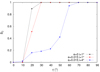 |
Fig. 14 Probabilities of capture of Phobos in the ν2 resonance with respect to the obliquity of the equator of Mars for different initial eccentricities and inclinations. |
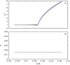 |
Fig. 15 Evolution of the inclination (a), and of the eccentricity (b) during the capture in the ν2 resonance for an obliquity of ε = 20° with the initial conditions e = 0.015 and Ω = 0°. The blue curve corresponds to the stable fixed point of the ν2 resonance computed with Eq. (37). |
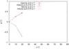 |
Fig. 16 Evolution of the maximum and minimum variations Δi in the mean inclination owing to the encounter with the ν2 resonance inthe case where the capture fails, with respect to the obliquity for different initial eccentricities. |
6.4.2 Inclination variation
In Fig. 16, we show the evolution of the mean inclination during the crossing of the ν2 resonance when the capture does not occur. We only plot the results for the obliquities 0°, 10°, and 20°, because for values of the obliquity larger than 30° the capture always occurs. As for the ν1 resonance, the amplitude of the variation increases with the obliquity. However, we did not observe any significant variation in the eccentricity during the crossing of the ν2 resonance.
7 Conclusion
In this paper, we have revisited the secular dynamics of a satellite while perturbed by the orbital motion of its planet. Previous studies have shown that some of these resonances can significantly modify the eccentricity (evection-like resonance) or the inclination (eviction-like resonance) of a satellite (e.g., Yoder 1982; Touma & Wisdom 1998; Yokoyama 2002; Yokoyama et al. 2005). Eviction-like resonances are important to map, because the inclination can be used to put constrains on the formation of the satellite. Moreover, some eviction-like resonances can be present even for the nearly zero eccentricities currently observed for the main satellites of the solar system planets.
Capture in eviction-like resonances is a possibility when the semi-major axis of the planet is decreasing. This capture can lead to a significant increase in the inclination of the satellite. However, for nearly zero eccentricity, capture is only possible in two of these resonances that we dubbed ν1 and ν2. These resonances are placed close to the planets’ surface, and only satellites spiraling into the planet may be affected, such as Phobos or Triton. We analytically compute the capture probability in the ν1 resonance and compare it to numerical simulations. We have shown that the evolution of Phobos cannot be considered as adiabatic.
When the eccentricity of the satellite is nonzero, evection-like and additional eviction-like resonances are possible. Some of these resonances are close to each other, and they can interact between them. We have studied these interactions with the method of frequency map analysis that can be used as an alternative to surface sections, since it is easier to implement in problems with many degrees of freedom. In the case of the ν1 resonance, we confirm that the interaction with the evection resonance νe introduces a chaotic region around the ν1 resonance (Yokoyama 2002; Yokoyama et al. 2005). In the case of Phobos, for eccentricities larger than 0.05, the evection resonance completely destroys the stability of the ν1 resonance and capture is no longer possible. In addition, because the evection resonance occurs almost simultaneously with the ν1 resonance, a satellite that is spiraling into the planet will have its eccentricity excited by the evection resonance, which in turn decreases the chances of capture in the ν1 eviction-like resonance.
When the orbit of the satellite crosses a given secular resonance, capture is not certain. For eviction-like resonances, the probability of capture increases with the obliquity of the planet and decreases with the inclination of the satellite. When capture fails, the inclination of the satellite still undergoes some changes, although much smaller than in the capture scenario, and it can either increase or decrease. In the case of the ν1 resonance, the capture probability also strongly depends on the eccentricity. However, this is a collateral effect that results from the proximity of the nearby evection resonance.
We apply our model to the study of Phobos, whose orbit will be modified in the future due to the encounters with the ν1 and ν2 eviction-like resonances. We obtain for the capture probabilities similar results to Yokoyama (2002). The capture in the ν1 resonance is almost impossible, given the present obliquity of Mars and the present eccentricity of Phobos. Nevertheless, the crossing of this resonance can lead to variations in the inclination between − 0.08° and 0.07°. On the contrary, capture in the following ν2 resonance is almost certain if the obliquity of Mars and the inclination of Phobos are similar to the current values, which will lead to a continuous increase in the inclination. If the capture fails, the crossing of the ν2 resonance can lead to variations in the inclination between −0.7° and 0.4°.
We have seen that secular resonances due to stellar perturbations, such as evection-like and eviction-like resonances, can significantly influence the motion of a satellite. The effect of planetary perturbations on satellite orbits are often considered as negligible, but they also induce secular resonances, whose crossings can lead to a one-time variation in the eccentricity or the inclination. If the perturbations are strong enough, captures in these resonances could also be possible, and induce more significant changes. Future studies on the orbital evolution of satellite orbits should thus also estimate the effect from these additional secular resonances.
Acknowledgements
This work was supported by CIDMA (UIDB/04106/2020 and UIDP/04106/2020), CFisUC (UIDB/04564/2020 and UIDP/04564/2020), PHOBOS (POCI-01-0145-FEDER-029932), ENGAGE SKA (POCI-01-0145-FEDER-022217), and GRAVITY (PTDC/FIS-AST/7002/2020), funded by COMPETE 2020 and FCT, Portugal.
References
- Agnor, C. B., & Hamilton, D. P. 2006, Nature, 441, 192 [NASA ADS] [CrossRef] [Google Scholar]
- Batygin, K., & Morbidelli, A. 2020, ApJ, 894, 143 [NASA ADS] [CrossRef] [Google Scholar]
- Borderies, N., & Goldreich, P. 1984, Celest. Mech., 32, 127 [NASA ADS] [CrossRef] [Google Scholar]
- Boué, G., & Laskar, J. 2006, Icarus, 185, 312 [Google Scholar]
- Canup, R. M. 2005, Science, 307, 546 [NASA ADS] [CrossRef] [Google Scholar]
- Canup, R. M., & Asphaug, E. 2001, Nature, 412, 708 [Google Scholar]
- Carvalho, J. P. S., & Vilhena de Moraes, R. 2020, Eur. Phys. J. Special Top., 229, 1491 [NASA ADS] [CrossRef] [Google Scholar]
- Chandrasekhar, S. 1987, Ellipsoidal figures of equilibrium [Google Scholar]
- Chirikov, B. V. 1979, Phys. Rep., 52, 263 [NASA ADS] [CrossRef] [Google Scholar]
- Correia, A. C. M. 2009, ApJ, 704, L1 [NASA ADS] [CrossRef] [Google Scholar]
- Couetdic, J., Laskar, J., Correia, A. C. M., Mayor, M., & Udry, S. 2010, A&A, 519, A10 [NASA ADS] [CrossRef] [EDP Sciences] [Google Scholar]
- Dumas, H. S.,& Laskar, J. 1993, Phys. Rev. Lett., 70, 2975 [NASA ADS] [CrossRef] [Google Scholar]
- Efroimsky, M., & Lainey, V. 2007, J. Geophys. Res. (Planets), 112, 12003 [CrossRef] [Google Scholar]
- Farago, F., & Laskar, J. 2010, MNRAS, 401, 1189 [Google Scholar]
- Frouard, J., Fouchard, M., & Vienne, A. 2010, A&A, 515, A54 [NASA ADS] [CrossRef] [EDP Sciences] [Google Scholar]
- Goldreich, P. 1965, AJ, 70, 5 [NASA ADS] [CrossRef] [Google Scholar]
- Henrard, J. 1982, Celest. Mech., 27, 3 [Google Scholar]
- Henrard, J. 1993, The Adiabatic Invariant in Classical Mechanics, eds. C. K. R. T. Jones, U. Kirchgraber, & H. O. Walther (Berlin, Heidelberg: Springer Berlin Heidelberg), 117 [Google Scholar]
- Inderbitzi, C., Szulágyi, J., Cilibrasi, M., & Mayer, L. 2020, MNRAS, 499, 1023 [NASA ADS] [CrossRef] [Google Scholar]
- Jacobson, R. A. 2010, AJ, 139, 668 [Google Scholar]
- Jacobson, R. A., & Lainey, V. 2014, Planet. Space Sci., 102, 35 [CrossRef] [Google Scholar]
- Kinoshita, H. 1993, Celest. Mech. Dyn. Astron., 57, 359 [NASA ADS] [CrossRef] [Google Scholar]
- Konopliv, A. S., Park, R. S., & Folkner, W. M. 2016, Icarus, 274, 253 [Google Scholar]
- Lambeck, K. 1979, J. Geophys. Res., 84, 5651 [NASA ADS] [CrossRef] [Google Scholar]
- Laskar, J. 1988, A&A, 198, 341 [NASA ADS] [Google Scholar]
- Laskar, J. 1990, Icarus, 88, 266 [NASA ADS] [CrossRef] [Google Scholar]
- Laskar, J. 1993, Physica D, 67, 257 [NASA ADS] [CrossRef] [Google Scholar]
- Laskar, J. 2003, ArXiv e-prints, [arXiv:math/0305364] [Google Scholar]
- Laskar, J., & Robutel, P. 1993, Nature, 361, 608 [Google Scholar]
- Laskar, J., Froeschlé, C., & Celletti, A. 1992, Physica D, 56, 253 [NASA ADS] [CrossRef] [Google Scholar]
- Laskar, J., Correia, A. C. M., Gastineau, M., et al. 2004, Icarus, 170, 343 [NASA ADS] [CrossRef] [Google Scholar]
- Nesvorný, D., Vokrouhlický, D., & Morbidelli, A. 2007, AJ, 133, 1962 [CrossRef] [Google Scholar]
- Smart, W. M. 1953, Celestial Mechanics (London, New York: Longmans, Green) [Google Scholar]
- Szeto, A. M. K. 1983, Icarus, 55, 133 [CrossRef] [Google Scholar]
- Touma, J., & Wisdom, J. 1993, Science, 259, 1294 [NASA ADS] [CrossRef] [Google Scholar]
- Touma, J., & Wisdom, J. 1998, AJ, 115, 1653 [NASA ADS] [CrossRef] [Google Scholar]
- Tremaine, S., Touma, J., & Namouni, F. 2009, AJ, 137, 3706 [Google Scholar]
- Ward, W. R. 1979, J. Geophys. Res., 84, 237 [NASA ADS] [CrossRef] [Google Scholar]
- Xu, W., & Fabrycky, D. 2019, AJ, submitted [arXiv:1904.02290] [Google Scholar]
- Yoder, C. F. 1979, Celest. Mech., 19, 3 [NASA ADS] [CrossRef] [Google Scholar]
- Yoder, C. F. 1982, Icarus, 49, 327 [CrossRef] [Google Scholar]
- Yokoyama, T. 2002, Planet. Space Sci., 50, 63 [CrossRef] [Google Scholar]
- Yokoyama, T., Mana, M. R., do Nascimento, C., Santos, M. T., & Callegari, N., J. 2005, A&A, 429, 731 [NASA ADS] [CrossRef] [EDP Sciences] [Google Scholar]
We analyze the quantity  , where k′ = (kx, ky, kz) corresponds to the coordinates of the normal to the satellite’s orbit expressed in the referential of the equator of the planet. In the quasi-periodic approximation, the precession frequency corresponds to the main frequency with the largest amplitude.
As the location of the stable point of the ν1 resonance depends on the eccentricity (Eq. (27)), and also on the considered Hamiltonian, we need to slightly modify the value of the semi-major axis in order that the location of the stable point is located about at the same place for each eccentricity and Hamiltonian.
Following Couetdic et al. (2010), we estimate the diffusion σ′ for a shorter interval [0 : T′], where T′ = T∕100. In general, for a stable trajectory σ < σ′, because the accuracy of the frequency analysis increases with the size of the interval, while σ > σ′ for an unstable trajectory, as the chaotic diffusion increases with time. We then construct the histogram of the trajectories verifying σ < σ′ with a step of 0.5. The values of σ and σ′ are averaged over the closest neighbors of the grid of initial conditions to decrease the effects of chaotic trajectories which have small values of the diffusion. From this histogram, we determine with a linear interpolation the value log10σs = −4.4 below which 99% of the trajectories verify σ < σ′.
For the maps with e = 0.03 and e = 0.045 in Fig. 7, some black regions appear around i = 0° and i = 1° that do not correspond to the ν1 resonance. They correspond to stable circulation regions that incidentally also have θ < θr.
We do not have many examples for the initial eccentricity 0.015 after capture, because the probability is very small.
All Tables
All Figures
|
Fig. 1 Jacobi coordinates, where r is the position of m relative to m1 (satellite orbit), and r1 is the position of the center of mass of m and m1 relative to m0 (planet orbit). The planet is a rigid body, where S is the rotational angular momentum. |
| In the text | |
|
Fig. 2 Orbital elements of the orbit of the satellite (in red). |
| In the text | |
|
Fig. 3 Level curves of the Hamiltonian (24) for Phobos (Table 1), for a semi-major axis a = 2.61686 R, and assuming an obliquity ε = 90° for Mars. |
| In the text | |
|
Fig. 4 Evolution of the inclination of Phobos for the stable fixed points with respect to its semi-major axis for the ν1 resonance (red curve) computed with Eq. (27), and for the ν2 resonance(blue curve) computed with Eq. (37) for a Martian obliquity of ε = 25°. The Roche limit for Phobos is a∕R ≈ 1.6. |
| In the text | |
|
Fig. 5 Capture probability of Phobos in the ν1 resonance with respect to the obliquity of Mars. The black curve corresponds to the capture probability computed with Eq. (52). The blue crosses and the red dots correspond to the capture probability determined for each value of the obliquity with N = 720 numericalintegrations of the resonant Hamiltonian (Eq. (19)), respectively with Q = 99.5 and Q = 5000 for the effective specific tidal dissipation. The errorbars are given by |
| In the text | |
|
Fig. 6 Capture probability of Phobos in the ν1 resonance with respect to the obliquity of Mars for different orbital parameters of Phobos. The black line corresponds to the current parameters. |
| In the text | |
|
Fig. 7 Stability maps for Phobos (Table 1) using an obliquity for Mars ε = 90°. From top to bottom, the initial eccentricity is e = 10−5, e = 0.015, e = 0.03, e = 0.045. Each column corresponds to the integration using different Hamiltonians: resonant Hamiltonian (left), interaction Hamiltonian (middle) and the full secular Hamiltonian (right). The color scale indicates the value of the quantity log10 σ. The blue and green areas correspond to stable circulating trajectories, while the yellow, orange, and red ones correspond to chaotic motions. The black areas correspond to stable resonant regions, for which log10 θ < −3.9. |
| In the text | |
|
Fig. 8 Capture probabilities of Phobos in the ν1 resonance with respect to the obliquity of the equator of Mars for different initial eccentricities. |
| In the text | |
|
Fig. 9 Evolution of the inclination (a) and of the eccentricity (b) during the capture in the ν1 resonance for an obliquity of ε = 90° with the initial conditions e = 0.015 and Ω = 351.5°. The blue curve corresponds to the stable fixed point of the ν1 resonance computed with Eq. (27). |
| In the text | |
|
Fig. 10 Evolution of the inclination (a) and of the eccentricity (b) during the crossing of the ν1 resonance for an obliquity of ε = 60° with the initial conditions e = 0.015, and Ω = 231°. |
| In the text | |
|
Fig. 11 Evolution of the inclination (a) and of the eccentricity (b) during the crossing of the ν1 resonance for an obliquity of ε = 60° with the initial conditions e = 0.015, and Ω = 203°. |
| In the text | |
|
Fig. 12 Evolution of the maximum and minimum variations in the mean eccentricity Δe owing to the encounter with the ν1 resonance in the cases where the capture in the resonance fails (a), and succeeds(b), with respectto the obliquity for different initial eccentricities. |
| In the text | |
|
Fig. 13 Evolution of the maximum and minimum variations in the mean inclination Δi owing to the encounter with the ν1 resonance in the case where the capture in the resonance fails, with respect to the obliquity for different initial eccentricities. |
| In the text | |
|
Fig. 14 Probabilities of capture of Phobos in the ν2 resonance with respect to the obliquity of the equator of Mars for different initial eccentricities and inclinations. |
| In the text | |
|
Fig. 15 Evolution of the inclination (a), and of the eccentricity (b) during the capture in the ν2 resonance for an obliquity of ε = 20° with the initial conditions e = 0.015 and Ω = 0°. The blue curve corresponds to the stable fixed point of the ν2 resonance computed with Eq. (37). |
| In the text | |
|
Fig. 16 Evolution of the maximum and minimum variations Δi in the mean inclination owing to the encounter with the ν2 resonance inthe case where the capture fails, with respect to the obliquity for different initial eccentricities. |
| In the text | |
Current usage metrics show cumulative count of Article Views (full-text article views including HTML views, PDF and ePub downloads, according to the available data) and Abstracts Views on Vision4Press platform.
Data correspond to usage on the plateform after 2015. The current usage metrics is available 48-96 hours after online publication and is updated daily on week days.
Initial download of the metrics may take a while.