| Issue |
A&A
Volume 656, December 2021
|
|
|---|---|---|
| Article Number | A131 | |
| Number of page(s) | 14 | |
| Section | Stellar atmospheres | |
| DOI | https://doi.org/10.1051/0004-6361/202142175 | |
| Published online | 13 December 2021 | |
Simulations of the line-driven instability in magnetic hot star winds
Institute of Astronomy,
KU Leuven,
Celestijnenlaan 200D,
3001
Leuven,
Belgium
e-mail: This email address is being protected from spambots. You need JavaScript enabled to view it.
Received:
8
September
2021
Accepted:
7
October
2021
Abstract
Context. Line-driven winds of hot, luminous stars are intrinsically unstable due to the line-deshadowing instability (LDI). In non-magnetic hot stars, the LDI leads to the formation of an inhomogeneous wind consisting of small-scale, spatially separated clumps that can have great effects on observational diagnostics. However, for magnetic hot stars the LDI generated structures, wind dynamics, and effects on observational diagnostics have not been directly investigated so far.
Aims. We investigated the non-linear development of LDI generated structures and dynamics in a magnetic line-driven wind of a typical O-supergiant.
Methods. We employed two-dimensional axisymmetric magnetohydrodynamic simulations of the LDI using the Smooth Source Function approximation for evaluating the assumed one-dimensional line force. To facilitate the interpretation of these magnetic models, they were compared with a corresponding non-magnetic LDI simulation as well as a magnetic simulation neglecting the LDI.
Results. A central result obtained is that the wind morphology and wind clumping properties change strongly with increasing wind-magnetic confinement. Most notably, in magnetically confined flows, the LDI leads to large-scale, shellular sheets (‘pancakes’) that are quite distinct from the spatially separate, small-scale clumps in non-magnetic line-driven winds. We discuss the impact of these findings for observational diagnostic studies and stellar evolution models of magnetic hot stars.
Key words: radiation: dynamics / magnetohydrodynamics (MHD) / instabilities / stars: early-type / stars: winds, outflows
Current address: National Solar Observatory, 22 Ohi’a Ku St., Makawao, HI 96768, USA.
© ESO 2021
1 Introduction
Modern spectropolarimetric surveys employing the Zeeman splitting in spectral lines have firmly established that hot, luminous (OB) stars can harbour global surface magnetic fields. These surface magnetic fields are mainly dipolar and have field strengths ranging from a few 100 G to some 10 kG. Based on the current observational detection threshold, recent surveys show that only a modest fraction (≈7%) of Galactic single and binary OB stars harbour such surface magnetic fields (Fossati et al. 2015 (BOB); Alecian et al. 2015 (BinaMIcS); Wade et al. 2016; Petit et al. 2019 (MiMeS)), while outside the Galaxy there is not enough direct empirical evidence for magnetic OB stars yet (Bagnulo et al. 2020). The origin of these surface magnetic fields remains elusive, but the rarity of magnetic OB stars and the lack of short-term observed evolution of their magnetic field does not favour a dynamo mechanism as is, an example being the case of the Sun. Instead the prevailing thought is that the magnetic fields of magnetic OB stars are fossil fields stemming from earlier stellar phases (Borra et al. 1982; Alecian et al. 2019). In particular, recent research shows that proto-stellar mergers might offer a tentative explanation for surface magnetic fields in hot stars (Schneider et al. 2019, 2020).
The presence of a global stellar magnetic field can have important effects in governing the stellar wind of hot stars (Shore & Brown 1990; Babel & Montmerle 1997; Owocki & ud-Doula 2004). With the seminal work of Castor et al. (1975, hereafter CAK), it is known that OB stars drive strong line-driven winds due to the scattering of the stellar continuum radiation in a large ensemble of spectral lines and it has become the de facto standard for time-dependent wind models (e.g. Blondin et al. 1990; Cranmer & Owocki 1995; Kee et al. 2016; El Mellah & Casse 2017; Dyda & Proga 2018; Schrøder et al. 2021).
To that end, initial time-dependent two-dimensional magnetohydrodynamic (MHD) line-driven wind models also adopted CAK theory. Specifically these models have shown that the outwards expanding stellar wind can be magnetically channelled thereby forming a region of magnetically confined material, or, a circumstellar magnetosphere (ud-Doula & Owocki 2002). This kind of ‘inside-out expansion’ of the wind makes stellar magnetospheres fundamentally different from planetary magnetospheres that are due to ‘outside-in compression’ from the solar wind. Moreover, with the help of the so-called magnetic confinement–rotation diagram (Petit et al. 2013), it is possible to classify OB star magnetospheres based on magnetic and rotational properties. This leads to a distinction between fast rotating, strongly magnetic hot stars with centrifugal magnetospheres (CM; Townsend & Owocki 2005) and slowly rotating, moderately magnetic hot stars with dynamical magnetospheres (DM; Sundqvist et al. 2012b).
The use of CAK theory together with state-of-the-art spectropolarimetric observations have thus played a major role in enhancing the understanding of circumstellar magnetospheres of OB stars. However, a key limitation of these models is that they use CAK theory, which relies on the Sobolev approximation to compute the radiative acceleration of the wind (Friend & MacGregor 1984; ud-Doula & Owocki 2002; Townsend & Owocki 2005; Townsend et al. 2007; ud-Doula et al. 2008, 2009; Bard & Townsend 2016; Küker 2017; Daley-Yates et al. 2019). In the Sobolev approximation it is assumed that the interaction of photons and spectral lines is described in a purely local fashion (Sobolev 1960) with the important corollary that the stellar wind remains smooth and homogeneous and only external effects can break the smoothness (e.g. magnetic fields or rapid rotation).
In fact, it is nowadays well known that line-driven winds of non-magnetic hot stars are intrinsically inhomogeneous. The Doppler effect enhances small-scale velocity perturbations and exposes a spectral line to fresh, unattenuated continuum photons thereby leading to a runaway effect, or line-deshadowing instability (LDI) (MacGregor et al. 1979; Carlberg 1980; Owocki & Rybicki 1984). The LDI, however, is triggered on small spatial scales not covered within the Sobolev approximation. Time-dependent radiation-hydrodynamic simulations of the LDI show that once this instability is triggered a vigorous growth occurs leading to large non-linearities. The transition from the (microscopic) linear to the (macroscopic) non-linear regime is very subtle and the LDI is subject to wave-stretching (Feldmeier & Thomas 2017). Once in the non-linear regime the characteristic wind morphology becomes that of slow, overdense, clumpy structures embedded in a fast, rarefied medium (Owocki et al. 1988; Feldmeier 1995; Runacres & Owocki 2002; Dessart & Owocki 2005; Sundqvist et al. 2018; Driessen et al. 2019a; Lagae et al. 2021). The presence of such wind clumps is able to explain several observational phenomenae across the electromagnetic spectrum (Puls et al. 2008, for a review), and, especially, the clumps have a range of important effects on the interpretation of observational diagnostics (e.g. Puls et al. 2015).
For magnetic line-driven winds the effects of the LDI are poorly understood both from a theoretical and observational point-of-view. To date the only attempt to theoretically study the LDI in a magnetic line-driven wind is Driessen et al. (2020), who performed a three-dimensional linear stability analysis of magneto-radiative waves in a magnetic line-driven wind. A key insight from this study is that scattered photons provide a strong damping mechanism for short-wavelength, radially propagating magnetic waves in the wind. The exact effects of this damping on the non-linear wind dynamics and its potential observational signature remain to be investigated and necessarily require multi-dimensional radiation-MHD simulations.
In this paper we present the first effort in performing two-dimensional radiation-MHD simulations of the LDI. In particular, Sect. 2 presents the underlying computational details we have employed in our modelling. Our results regarding wind morphology and statistical properties are discussed within Sect. 3. We also briefly discuss the potential observational signatures of the LDI in a magnetic line-driven wind and frame our results with respect to stellar evolution models of magnetic hot stars (Sect. 4). Finally, Sect. 5 summarises our findings and suggests directions for further research. To gain further insight, Appendix B briefly compares our magnetic LDI wind models with previous wind models employing the CAK line-force parametrisation for the radiative acceleration.
2 Modelling of magnetic line-driven winds
2.1 Magnetic characterisation and adopted models
The important competition between the stellar wind and the magnetic field can be conveniently described by comparing their energies, that is wind kinetic energy vs. magnetic energy, and is quantified with a dimensionless quantity
 (1)
(1)
called the wind-magnetic confinement parameter (ud-Doula & Owocki 2002). In terms of this parameter, η⋆ ≫ 1 means a dominating magnetic field over the wind flow at the stellar surface and η⋆ ≪ 1 vice versa. It is set by the stellar magnetic field strength in the equator B⋆ = Bp∕2 in terms of the polar magnetic field strength Bp and the wind terminal momentum given by a mass-feeding rate ṀB = 0 (assumed tobe the mass-loss rate of an equivalent non-magnetic star) at terminal wind speed v∞.
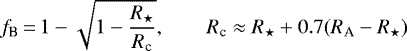
If confinement occurs this is over a constricted spatial extent since the magnetic energy always falls off faster than the wind energy (e.g. for observed dipole fields B ∝ 1∕r3, Grunhut et al. 2017). For a prototypical line-driven wind the spatial point where the wind starts to dominate is about
 (2)
(2)
also known as the Alfvén radius (ud-Doula & Owocki 2002). Because we do not consider rotation (see below), the Alfvén radius is theonly characteristic magnetosphere scale in the present work. This means that the magnetospheres here are Dynamical Magnetospheres (DM). Consulting the magnetic confinement–rotation diagram these are intrinsic to slowly rotating magnetic O-stars (Petit et al. 2013). Therefore, for our modelling we adopt stellar and wind parameters typical to a O-supergiant in the Galaxy as collected in Table 1.
Since the present work is concerned with a first study of a more complete description of the radiation line force in a magnetic line-driven wind this warrants some simplifications for other physics. We assume an isothermal wind fixed at the stellar effective temperature, that is heating from shocks is radiated away in an unresolved small cooling layer (Feldmeier et al. 1997; Lagae et al. 2021). Similarly, we do not consider additional effects such as (rapid) stellar rotation (ud-Doula et al. 2006, 2008), or an oblique dipolar magnetic field topology (Daley-Yates et al. 2019) that necessarily require a three-dimensional model.
Overview of parameters used in this work.
2.2 Magnetohydrodynamics
The employed conservative single-fluid, ideal magnetohydrodynamic (MHD) equations solve for the mass density ρ, velocity field v, and magnetic field B
 (3)
(3)
![Mathematical equation: \begin{equation*}\frac{\partial (\rho\mathbf{v})}{\partial t} + \nabla \cdot \left[\rho\mathbf{v}\mathbf{v} + \left(p + \frac{\mathbf{B}\cdot \mathbf{B}}{2}\right)\mathbf{I} - \mathbf{B}\mathbf{B} \right] \,{=}\, \rho\mathbf{g}_{\textrm{eff}}+ \rho\mathbf{g}_{\textrm{line}},\end{equation*}](/articles/aa/full_html/2021/12/aa42175-21/aa42175-21-eq4.png) (4)
(4)
 (5)
(5)
These are complemented with the divergence-free constraint
 (6)
(6)
and isothermal closure relation for the gas pressure
 (7)
(7)
with a the isothermal speed of sound defined from the stellar effective temperature, namely from assuming Twind = Teff, and Boltzmann’s constant kB for a gas with mean atomic weight m. We point out that in this formulation of the (dimensionless) equations the magnetic field is defined such that the magnetic permeability is μ0 = 1.
Additional source terms are included in the momentum equation to account for stellar gravity and the radiation force consisting of continuum and line interactions. In hot star winds the continuum force is primarily due to electron scattering, which effectively lowers gravity, such that it is customary to formulate both quantities together into an effective stellar gravity
 (8)
(8)
with Γe ≡ κeL⋆∕(4πGM⋆c) the Eddington factor for constant electron scattering with opacity κe = 0.34 cm2 g−1 (assuming full ionisation at solar abundances). The force due to lines, gline, is the important quantity in modelling a line-driven wind and will be detailed next.
2.3 Radiation line force
A key difference with previous work on magnetic line-driven winds is that we depart from the line force description gline within the Sobolev approximation (CAK, but see Appendix B for a comparison). However, with the added complexity of the line force description we still opt to treat the radiation transport by calculating it along an isolated one-dimensional ray within each colatitudinal cone of the simulation domain. In that respect our approach is the magnetic equivalent of the hydrodynamic models performed by Dessart & Owocki (2003).
The total line force (per unit mass) consists of direct and diffuse contributions due to photon absorption and scattering: gline ≡ gdir + gdiff. In driving the wind many lines participate and the cumulative contribution of all lines is described by an ensemble power-law distribution (CAK) in line strength q (Gayley 1995) with an additional exponential cut-off (Owocki et al. 1988) limiting the distribution to a line with maximum strength Qmax: N(q) ∝ qα−2 exp(−q∕Qmax), with α the power-law index of the assumed line distribution.
Within the non-Sobolev, Smooth Source Function approach (SSF, Owocki & Puls 1996) the ensemble-integrated direct and diffuse forces evaluate to
 (9)
(9)
 (10)
(10)
with optically thin line force and optically thin source function
 (11)
(11)
and  is a line-strength normalisation describing the ratio of the total line force to the force due to electron scattering if all lines were to be optically thin (Gayley 1995).
Formally the angle quadrature in Eq. (9) is to be computed over a bundle of radiation rays that intercept the stellar disc at  (thereby covering the full stellar disc) with direction cosine
  relative to the local direction at radius r. Such an approach is, however, computationally expensive and, instead, we only apply radial radiation rays within each separate latitudinal cell. Nonetheless, this single-ray quadrature is not truly radial since each ray is additionally weighted with y = 0.5 to mimic the finite extent of the stellar disc (Sundqvist & Owocki 2013)1. To avoid further computational complexity, the single-ray quadrature is also assumed for the diffuse radiation, Eq. (10), in a two-stream approximation for outward (‘+’) and inward (‘−’) directed radiation.
Along the ray the line-force components are computed using an ensemble-escape probability
 (12)
(12)
that takes into account the accumulated optical depth
 (13)
(13)
with Γ(α) the Gamma function, κ a frequency-integrated line opacity, and ϕ a Gaussian line-profile function at observer’sframe frequency x ≡ (ν∕ν0 − 1)c∕vth. With this definition,  in Eq. (12) denotes the optical depth of a line with strength
  . To capture the resonance zones in the wind acceleration region these optical depth integrals are solved by analytic integration between discrete grid points using linear interpolation in density and velocity (see Feldmeier & Thomas 2017, their Eqs. (7)–(8) for a similar approach).
2.4 Numerical specifications
To perform non-linear simulations of magnetic LDI winds we use the open-source2, parallel, grid-adaptive astrophysical (M)HD code MPI-AMRVAC (Xia et al. 2018; Keppens et al. 2021). Specifically, Eqs. (3)–(6) are solved in an unsplit fashion using a HLL Riemann solver (Harten et al. 1983) complemented with a parabolic spatial reconstruction scheme (PPM, Colella & Woodward 1984) and third-order accurate total-variation-diminishing Runge–Kutta temporal discretisation (Gottlieb & Shu 1998). For stability the time step is taken as the minimum of a fixed Courant time set to be 0.3 and an additionally computed time step due to the radiation and gravity force in Eq. (4) (see Eq. (8) in Lagae et al. 2021).
2.4.1 Simulation grid
The simulation spans the two-dimensional meridional (r, θ) plane and covers a radial extent r ∈ [R⋆, 6R⋆] and colatitudinal extent θ ∈ [0, π]. To resolve the steep wind acceleration region near the stellar surface, we stretch the radial grid away from the stellar surface with a factor Δri+1∕Δri = 1.002 between subsequent radial zones i and i + 1. In colatitude we assume uniform spacing Δθj.
This grid choice ensures that the Alfvén radius is sufficiently far from the outer boundary while the stretching allows us to resolve the barometric scale height of the photosphere,  , and the small spatial scales over which the instability operates. The latter implies resolving the radial Sobolev length LSob,r ≡ vth∕(dvr∕dr) ≈ (vth∕v)r ≈ 0.01 R⋆, for which we adopt nr = 1000 radial zones. Similarly, we also resolve a characteristic lateral Sobolev length, LSob,θ∕r = vth∕vr ≈ 0.5°, by using nθ = 384 zones in colatitude. As demonstrated by linear stability analysis, the flow should be stable on scales smaller than the lateral Sobolev length (Driessen et al. 2020).
2.4.2 Initial and boundary conditions
We initialise the line-driven wind model by starting from a relaxed one-dimensional spherically symmetric CAK wind that is distributed over the meridional plane. The poloidal velocity vθ (r, θ) = 0 initially. The magnetic field is taken to be a pure dipole with polar field strength Bp,
 (14)
(14)
The outer (supersonic, super-Alfvénic) radial boundary assumes that all hydrodynamic variables are continuous. At the lower boundary (stellar surface) the density ρ0 is fixed at five times the sonic point density in order to have a subsonic flow with a typical one-dimensional non-magnetic CAK mass flux. The radial velocity vr is extrapolated into the first ghost cell, allowing the wind to dynamically adjust while the remaining ghost cell values of vr are set equal to the first ghost cell. The radial magnetic field Br is fixed in the interior to enforce a dipolar field at the surface. The poloidal magnetic field Bθ is extrapolated into the ghost cells and the flow is forced along the magnetic field by fixing vθ. While the simulation adapts to its steady-state base outflow, we also prohibit the velocity to become supersonic at the lower boundary. We refer the reader to Appendix A for an extended account on the adopted boundary conditions.
Since the simulated meridional plane contains both polar axes (θ = 0 and θ = π) we employ π–boundary conditions in θ. Essentially this enforces that the fluid quantities are translated an amount π around the (singular) pole and vector quantities transform accordingly to allow for flow across the pole. This avoids numerical problems related to ill-defined geometric factors in divergence computations.
2.4.3 Treating the magnetic field and the monopole condition
The interaction of the LDI with the magnetic field can result in strong spatial gradients in the wind due to shock-dominated interactions. This often leads to numerical difficulties in solving the MHD equations, especially if the total magnetic field is solved for as the dependent variable. In order to circumvent such problems, we follow the method of Tanaka (1994), available in MPI-AMRVAC, and split the total dipole magnetic field B = B0 + δB in an intrinsic background dipole field B0 and a deviating field δB. This splitting off the total magnetic field B and only solving for the deviated field δB is more accurate and robust in regions of strong spatial gradients. Notice that here the background field is also potential-free (∇ × B0 = 0) and time-independent (although the method also works for time-dependent B0).
To make the magnetic field satisfy the divergence-free condition, Eq. (6), we apply the eight-wave scheme (Powell et al. 1999). Within this method any magnetic monopoles that arise in the simulation are advected away at the fluid velocity.
3 MHD simulation results
3.1 General wind properties
To gain insight in the non-linear evolution of the LDI with increasing magnetic confinement it is of interest to consider the wind density. In Fig. 1 we contrast a non-magnetic LDI model with weakly and strongly confined LDI models over several subsequent wind evolutionary times (t = 0, 50, 150, 300 ks).
Starting from a steady-state CAK wind, the non-magnetic LDI model develops a rather coherent wind structure initially (t <50 ks). However, the outwardly accelerating wind structure starts to become progressively disrupted due to Rayleigh–Taylor and thin-shell instabilities (Dessart & Owocki 2003) leading to the formation of spatially separated wind clumps. It is worth noting that in this non-magnetic wind model the lateral scale up to which LDI structure forms remains unclear. The fragmentation might result in large lateral scales due to lateral line drag acting on the flow (Rybicki et al. 1990; Driessen et al. 2020) or extend down to smaller lateral scales if, for example, the photosphere consists of many turbulent bubbles that leave their imprint in the wind. Within the one-dimensional SSF this break-up tends to happen up to the lateral Sobolev length such that a near complete lateral incoherence results in the wind. The resulting wind structure shows the typical characteristic slow, overdense clumps separated by a fast, rarefied interclump medium once settled in a ‘steady-state’ (Dessart & Owocki 2003; Sundqvist et al. 2018).
Furthermore since we assume a uniformly bright stellar disc and no photospheric perturbation (e.g. Sundqvist & Owocki 2013; Krtička & Feldmeier 2021) all LDI structure seen in our simulations is self-excited. It arises from the back-scattering of photons from the outer wind structure that seeds perturbations closer to the stellar surface which are subsequently amplified by the LDI (Dessart & Owocki 2003).
When introducing a weak magnetic field (i.e. weak confinement, η⋆ = 0.15) the overall picture is not significantly changed. Once sufficiently developed, however, the wind stretches the magnetic field into a nearly radial configuration that is reminiscent of a ‘split-monopole’. Along with this topology the formation of a current sheet occurs in the magnetic equatorial plane with a corresponding modest density enhancement. The morphology of the wind clumps remains also similar to the non-magnetic case showing that a weak magnetic field has a small effect on the clump dynamics.
The strongly confined LDI wind (η⋆ = 15) undergoes a markedly different dynamical evolution compared to the non-magnetic and weakly confined LDI wind. An important difference with respect to the other displayed models is the lack of lateral fragmentation and incoherence of the wind contrary to the standard non-magnetic LDI wind models hitherto performed (Dessart & Owocki 2003, 2005; Sundqvist et al. 2018). This happens particularly in the open field regions where the LDI generated structures manifest themselves as large-scale, wavy shellular sheets that advect outward at the local wind velocity. This suggests that the presence of a strong enough magnetic field makes the LDI unable to fragment into ‘wind clumps’ in this region, but rather transforms it into overdense ‘wind sheets’, still separated by a fast, very rarefied medium. It appears thus that the magnetic field stabilises against lateral plasma motions and forces all LDI structure along the magnetic field line (‘frozen-in flow’). Although the physical reasons for the underlying gas motions are different, this situation is quite similar to plasma flow in a sunspot where a strong vertical magnetic field inside the sunspot prohibits convective blobs from fragmenting into the lateral directions.
Additionally, after a long enough time, part of the wind plasma is guided along the magnetic field lines and confined over a small range in latitude by closed magnetic loops. The resulting circumstellar magnetosphere is akin to what has been found in previous magnetic wind studies using the CAK line force (ud-Doula & Owocki 2002, see also Appendix B). Indeed, plasma at higher latitudes is channelled towards the magnetic equator where collisions from opposite magnetic footprints happen and the resulting plasma compression leads to a rather slow, dense outflow. Most notably there are no signatures of the characteristic LDI structures within the circumstellar magnetosphere, although the wind is radiatively unstable in this region. The apparent absence of LDI-like structures in the magnetosphere might be due to a misalignment between local flow and magnetic field vectors that induces a growth restriction or the fact that higher density material falls back onto the star and dominates the LDI.
The appearance of wind sheets instead of wind clumps also suggests that the wind clumping and porosity properties (Owocki & Sundqvist 2018) in the open field regions of these magnetic LDI winds might be much different from their non-magnetic counterparts (e.g. Feldmeier et al. 2003; Sundqvist et al. 2012a, that consider LDI-like ‘shells’ and porosity in context of effects upon absorption of X-rays). What the exact effect of these large-scale shellular wind sheets is on observations remains to be investigated in detail. However, we discuss some first aspects of their presence in Sect. 4.
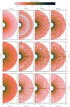 |
Fig. 1 Logarithmic wind density displaying the evolution in time for our adopted LDI models: (top) non-magnetic wind with η⋆ = 0, (middle) moderately confined wind with η⋆ = 0.15, and (bottom) strongly confined wind with η⋆ = 15. The overplotted white lines in the magnetic wind models represent streamlines to illustrate the magnetic field topology. |
3.2 Statistical properties
To further analyse the LDI structures in our models we consider statistical averages (here temporal averages) of hydrodynamic quantities. These statistics are computed from every numerical iteration beginning significantly after the simulation has developed its characteristic wind structure as set by the dynamical timescale τdyn = R⋆∕v∞≈ 10 ks. All computations start at tstat = 200 ks ≈ 20τdyn for each model such that statistical quantities span ≈ 100 ks ≈ 10τdyn within the simulations.
To emphasise similarities between our two-dimensional simulations and previous one-dimensional simulations (all treating the LDI line force in a one-dimensional fashion) we display in Fig. 2 a radial cut of wind velocity and density taken at an arbitrarily chosen colatitude θ away from the magnetosphere. In such an isolated colatitudinal cone the wind properties show the characteristic one-dimensional features of slow, overdense clumps (or shells) that are separated by a fast, nearly-void medium. However, with increasing magnetic confinement the radial velocity and density variations appear less strong. Since all parameters in the models are fixed, except for the polar magnetic field strength, this suggests that the increasing magnetic field strength reduces the strength of the LDI in a relative sense, and as can be seen, also the position at which it sets in.
Although the discussion so far applies to a single radial wind slice, these typical LDI features occur over a large portion of the wind. To illustrate this we take averages over latitude to recover a corresponding one-dimensional smooth velocity and density profile. In order to have a meaningful average in latitude the simulation domain is constrained to a 45° wedge near the pole to avoid material inside the spatial extent of the magnetosphere in the η⋆ = 15 case. For direct comparison this wedge is then adopted for each model discussed here. As displayed in Fig. 2 the corresponding smooth mean one-dimensional wind velocity and density describes well the variations in a randomly chosen radial cut. Hence, all radial cuts within the wedge display similar velocity and density variations around this mean and as such are prototypes of a corresponding one-dimensional LDI wind.
We also point out that under strong confinements the wind becomes faster. This effect is due to the faster-than-radial expansion of the field that results in higher velocities near the magnetic pole (Owocki & ud-Doula 2004). Since our wedge is defined near the pole region to leave out any magnetosphere contributions this effect manifests itself inherently in Fig. 2.
The reduction in LDI strength for increasing magnetic confinement is also seen when considering the velocity dispersion (Fig. 3) averaged over the wedge
 (15)
(15)
which is a good proxy for the reverse shock speed due to the LDI. Since the velocity dispersion relates to the velocity jumps due to shocks this shows that with increasing magnetic confinement the shocks become less strong, resulting in weaker wind density compressions, and to less overdense wind clumps (cf. Fig. 2).
In Fig. 4 we elaborate further on the η⋆ = 15 model and show first the wind clumping factor
 (16)
(16)
In non-magnetic hot stars wind clumping can seriously affect observational diagnostics depending on ρ2 -processes and leads to an overestimate of inferred mass-loss rates with a factor  . Corrections for fcl in non-magnetic hot stars can be obtained via multi-wavelength diagnostics or complex, time-dependent numerical simulations of the LDI. In particular, the optical diagnostic line Hα formed at r ≤ 2 R⋆ is often used as a mass-loss rate tracer for non-magnetic hot star winds and a typical wind clumping factor is fcl ≈ 10−20 (Puls et al. 2006; Najarro et al. 2011; Hawcroft et al. 2021; Rubio-Díez et al. 2021).
For magnetic hot stars, constraints on fcl are presently not well established. To that end in Fig. 4 we display the wind clumping cut off to a maximum of fcl = 10 (typical non-magnetic adopted Hα clumping factor) and wind clumping without cut off. Within the magnetosphere density enhancements provide regions with wind clumping fcl ≥ 10 due to fall-back of dense material from the magnetic equatorial plane. Outside the magnetosphere any wind clumping is due to the LDI which is comparatively lower in large portions of the unconfined wind.
Considering wind clumping in the magnetosphere is of interest for wind line-diagnostics such as Hα (more discussion in Sect. 4). The wind clumping displayed in Fig. 4 is calculated from a temporal average, and when further averaging this over the spatial extent of the magnetosphere, we find a modest wind clumping of fcl ≈ 4 inside the magnetosphere. It is likely that such temporal averaging underestimates density enhancements over long times (several hundred thousand iterations in our simulation). In a two-dimensional model there is only one azimuthal slice over which the average is continuously taken leading to a smooth density structure. In three-dimensional simulations, however, at any instant density structures will be arbitrarily distributed along the azimuth in time (ud-Doula et al. 2013; Daley-Yates et al. 2019). Therefore, we compute from fifty arbitrarily chosen snapshots a spatial average of wind clumping. Doing so results in magnetospheric wind clumping values of fcl ≈ 40 that is in good agreement with earlier attempts from magnetic line-driven wind models neglecting the LDI (Owocki et al. 2016; Driessen et al. 2019b).
Alongside fcl we also display in Fig. 4 the average radial and poloidal wind velocity. The radial velocity contours demonstrate that outside the magnetosphere the wind accelerates and averages out to a smooth wind with vr ≈ 2500 km s−1 with a faster flow near the pole (Owocki & ud-Doula 2004). Within the magnetosphere on average most material falls back onto the star while only a fraction of it escapes in the magnetic equatorial plane. Similarly, the poloidal velocities show that inside the magnetosphere material from opposite footprints is channelled towards the equatorial plane with vθ ≈ 700−800 km s−1. Outside the magnetosphere this poloidal velocity gradually decreases towards the pole as magnetic field lines become progressively radially stretched. These velocity contours reinforce that simply assuming a monotonic velocity profile in line-diagnostic studies leads to erroneous wind parameter estimates (e.g. Howarth et al. 2007; Martins et al. 2015a).
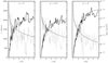 |
Fig. 2 Lateral averages of statistically computed wind velocity and wind density (dashed lines). Lateral averages are taken in a wedge near the pole (θ = 0−45°, to not have magnetosphere contamination) at simulation termination. Superimposed is a radial cut of wind velocity and density at an arbitrarily chosen colatitude θ within this wedge (solid lines). |
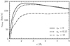 |
Fig. 3 Radial velocity dispersion laterally averaged over the wedge near the pole (θ = 0− 45°). |
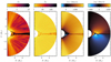 |
Fig. 4 Statistical contours (from left to right) of wind clumping restricted to a maximum of ten, full wind clumping, radial wind velocity, and poloidal wind velocity for a magnetically confined LDI wind with η⋆ = 15. |
3.3 Global mass-loss rate
For stars with magnetospheres the concept of ‘mass-loss rate’ requires attention because the magnetic channelling makes a significant fraction of material unable to escape the star. Therefore, the mass launched from the stellar surface is really a ‘mass-feeding rate’ ṀB = 0, which, here, is assumed to be the same mass loss a non-magnetic star undergoes. This quantity, however, can differ significantly from the actual, global mass-loss rate of the star ṀB. To first order both mass-loss rate quantities can be related to each other (ud-Doula et al. 2008) by taking into account the area the magnetosphere covers such that the fraction of open magnetic field lines amounts to
 (17)
(17)
and the global mass-loss rate ṀB scales as
 (18)
(18)
To verify this result, we compute global mass-loss rates from our simulations by considering how much mass is lost through the outer radial boundary. This means we compute in our simulation a mass flux  , weighted by sinθ, to average out the variability from the advection of the large-scale wind sheets.
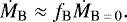
Figure 5 collects the computed global mass-loss rates and compares them with Eq. (18). Overall there is good agreement between the prediction of ud-Doula et al. (2008) and our numerical LDI simulations. Such an outcome demonstrates that the LDI force description, when averaged over long enough advection times, resembles well the ‘steady-state’ wind structures also appearing in magnetic CAK models to which ud-Doula et al. (2008) calibrated Eq. (18).
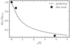 |
Fig. 5 Modulation of the global mass-loss rate ṀB with wind magnetic confinement |

3.4 Spatial coherence of wind clumps
To better illustrate the wind morphology in Fig. 6 we display a similar wind density state but now normalised as  for the non-magnetic and strongly confined LDI wind. Since the attained density contrasts can become quite large in a shocked LDI wind, the panels in Fig. 1 tend to underestimate the amount of structure in the wind (since they are shown at the same density scale). To that end a normalisation with respect to the mean wind density of each LDI model is more appropriate because wind variations occur with respect to this mean. Within this normalisation then the extended shellular-like nature of the wind clumps in the strongly confined LDI wind becomes more apparent showing that these wind sheets (‘pancakes’) can cover half a hemisphere of the star. On the contrary, the non-magnetic LDI wind still shows small-scale spatially separated wind clumps that tend to elongate at the outer radial boundary due to the spherical divergence.
 |
Fig. 6 Density contrast with respect to the average wind density for the non-magnetic and strongly confined LDI wind model. |
4 Discussion on observational signatures and stellar evolution
We discuss here some possibilities to disentangle the signatures of the wind sheets as found within the numerical simulations. We also comment onany effects of the predicted mass-loss rates and stellar evolution modelling of magnetic hot stars. The discussion focuses on the η⋆ = 15 LDI model since this is a reasonably realistic wind confinement for magnetic O-stars in the Galaxy.
4.1 Spectroscopy
Over the past decade it has been extensively demonstrated that the circumstellar magnetosphere is an excellent probe to infer several windand magnetospheric parameters of magnetic hot stars using X-rays (Nazé et al. 2010, 2012, 2016), resonance UV lines (Marcolino et al. 2013; Nazé et al. 2015; David-Uraz et al. 2019a; Erba et al. 2021), and optical recombination lines (Sundqvist et al. 2012b; Wade et al. 2012, 2015; ud-Doula et al. 2013; Owocki et al. 2016; Shultz et al. 2020). These prime diagnostic domains can be complemented with the infrared (Eikenberry et al. 2014; Oksala et al. 2015) and radio domain (Trigilio et al. 2004; Das et al. 2020).
The LDI generates strong reverse shocks that leads to X-ray emission in line-driven winds. In particular, magnetic O-stars are strong sources of soft X-ray emission (Nazé et al. 2014) that can naturally result from the wind sheets outside the magnetosphere. Nonetheless, it is worth noting that so far in all numerical models LDI generated shocks underestimate the amount of soft X-ray emission in non-magnetic line-driven winds (Feldmeier et al. 1997). Therefore, within the current modelling attempts, it is questionable whether the magnetic LDI models can correctly estimate the amount of soft X-ray emission for magnetic hot stars. On the other hand, it seems unlikely that the LDI contributes significantly to the generation of hard X-rays that are understood to emerge from shocks resulting from the collision of magnetically channelled flow (Babel & Montmerle 1997; Gagné et al. 2005).
The UVline column-mass dependency could provide insights into the advective motion of the wind sheets. This could appear quite similar, for example, to the discrete absorption components (DACs) that are seen in absorption troughs of UV P Cygni profiles of (magnetic) hot stars (Howarth & Prinja 1989; Kaper et al. 1996; Martins et al. 2015b; Sudnik & Henrichs 2016; David-Uraz et al. 2017). However, it is important to point out that such DACs are believed to be modulated by stellar rotation, whereas here we would expect variation on a dynamical advection timescale, which thus should be different. For stars viewed near their magnetic pole, the advective motion of the wind sheets can manifest itself in the absorption trough of such P Cygni profiles. Since the sheets typically traverse one stellar radius in a few hours this does require high-cadence and high-resolution spectroscopy assuming observational noise does not hide the signature. Further insights into this hypothesis, however, can be obtained using synthetic observations of UV resonance lines using state-of-the-art radiative transfer codes (e.g. Hennicker et al. 2020).
Finally, the Hα line-profile variability in magnetic hot stars stems naturally from the density structure within the magnetosphere (e.g. Sundqvist et al. 2012b). Since Hα is a recombination line the inference of mass-feeding rates crucially depends on the amount of wind clumping taken into account. For example, in non-magnetic hot stars the commonly adopted value is fcl = 10, but as seen in Fig. 4 such wind clumping factors can be much higher in the magnetically confined region. A typical spatial average of wind clumping inside the magnetosphere amounts to fcl ≈ 40 (but see discussion in Sect. 3.2). This vividly illustrates that applying typical wind clumping factors used for non-magnetic hot stars may provide erroneous estimates of the amount and effect of wind clumping. Consequently the mass-feeding rate of such magnetic hot stars may also be more reduced when compared with a non-magnetic counterpart. This reduction in mass-feeding rate can also have important effects on the stellar evolution and final fate of magnetic hot stars (see below).
4.2 Photometry and polarimetry
Current photometric data has shown to be another alternative to diagnose hot star magnetospheres (David-Uraz et al. 2019b; Munoz et al. 2020). Such photometric signatures might be harder to relate to an inhomogeneous wind, however, since other processes can disturb the signal (e.g. stellar pulsations or rotational modulations). For example, the wind sheet overdensities near the star can potentially be seen as semi-regular photometric variability. We expect this effect to be most pronounced near the magnetic pole of the star where the wind flow is mainly radial and does not suffer from magnetospheric contamination. Any possible photometric signatures would then quasi-periodically appear in the photometric data within a time span of several hours needed to advect outwards.
Due to the high degree of ionisation in line-driven winds measurements of continuum polarisation can provide another window for probing the existence of wind sheets. Indeed, the linearly polarised light due to electron scattering in these hot atmospherescan provide a clue into the geometrical distribution of the wind sheets, that is deviations from spherical symmetry.
4.3 Evolutionary modelling of magnetic hot stars
Determination of the mass-feeding rates versus the mass-loss rates of magnetic hot stars is of interest due to their potentially different evolutionary pathways compared to non-magnetic hot stars. Particularly, it has been shown that magnetic OB stars quench a large amount of their mass flux and could become progenitors of heavy stellar-mass black holes nowadays linked with gravitational wave detections (Petit et al. 2017).
In these stellar evolution models of magnetic hot stars the assumed mass-loss rate (i.e. the mass-feeding rate ṀB = 0) has been taken from corresponding non-magnetic OB star predictions (Vink et al. 2001). This ṀB = 0 is then linked via Eq. (18) to the globalmass-loss rate ṀB in such evolution models. However, it is worth noting that the recent line-driven wind models of Sundqvist et al. (2019) and Björklund et al. (2021) predict a factor three lower ṀB = 0 than Vink et al. (2001) in the O-star regime. Therefore, using these new O-star mass loss rate predictions would also reduce ṀB by a factor of three compared to what is currently employed in magnetic OB star evolution modelling (Petit et al. 2017; Georgy et al. 2017; Keszthelyi et al. 2019, 2020). Given the strong interdependence of mass loss rate and evolution for hot stars (Meynet & Maeder 2000), further studies are required to test the effects of this further reduction in mass-loss for magnetic OB stars.
It is important to recall that the inclusion of the LDI does not alter either the global mass-feeding rate as predicted from line-driven wind theory, nor the mass-loss rate predicted from magnetospheric confinement (see discussion surrounding Fig. 5). However, for observational modelling, constraints on wind clumping (inside and outside of the magnetosphere) are necessary to further understand and constrain both the mass-feeding and mass-loss rate of the star. For example, as discussed above, the validity of using non-magnetic mass-feeding rates in stellar evolution modelling is a priori not guaranteed due to the additional (unknown) complexities the magnetic field can exert on the mass flux. However, first empirical constraints from Hα line-profile modelling within the circumstellar magnetosphere, taking into account wind clumping corrections a posteriori, provide a tentative back-up for these non-magnetic mass-feeding rate adaptations (Driessen et al. 2019b). In particular, these authors demonstrated that for a selected sample of Galactic magnetic OB stars the adaptation of the Vink et al. (2001) mass-loss rates is justifiable if the global mass-loss rate ṀB is scaled down accordingly with a factor of fcl ≈ 50, which in light of the present study, aligns well with the results discussed in Sect. 3.2. Future extensions to this study in light of the wind clumping outside the magnetosphere found here could, however, test this finding with additional diagnostics.
5 Conclusions and future work
In this paper we have presented a first theoretical investigation into the wind ‘clumping’ properties of magnetic O-stars due to the line-deshadowing instability (LDI). In particular we have employed two-dimensional magnetohydrodynamic simulations whereby the radiation line force is still computed using the one-dimensional Smooth Source Function (SSF) approximation (Owocki & Puls 1996).
Our main result is that increasing the wind-magnetic confinement to values typically expected for magnetic O-stars, that is magnetically confined flows, leads to a two-state wind morphology; (i) in accordance with previous magnetic CAK wind models inside the circumstellar magnetosphere the flow is confined with regular wind flow fall-back towards the star, and (ii) outside the magnetosphere large-scale coherent, shellular ‘wind sheets’ separated by a rarefied medium advect outwards contrary to previous magnetic CAK and non-magnetic LDI wind models.
We are currently extending our radiation-MHD models to take into account a proper (although spatially restricted) description of the two-dimensional SSF radiation transport (Sundqvist et al. 2018). This allows us to further study the influence of strong magnetic fields and the fragmentation of LDI-like structures with the inclusion of non-radial line forces.
Among several proposed potential observational signatures, we are also investigating the effects of UV line-profile variability from LDI generated wind sheets using a state-of-the-art three-dimensional radiative transfer code (Hennicker et al. 2020). Since UV lines arecolumn-mass diagnostics the advection of overdense wind sheets near the pole might be seen within the absorption trough of a P Cygni profile. Whether such effect are observable, that is not dominated by noise, remains to be investigated. Results of these works will be reported in the future.
Overall the main conclusion of the present study is that LDI generated wind structure in a magnetically confined line-driven wind can differ significantly with non-magnetic LDI wind models, as well as with magnetic line-driven wind models that apply CAK theory for the description of the radiation line force (i.e. the intrinsic appearance of wind sheets due to the LDI not seen in the other models). With future research we intend to further investigate theoretical and observational aspects to test the signatures predicted from the present simulations and assess its predictive power and validity.
Acknowledgements
It is a pleasure to thank Stan Owocki and Asif ud-Doula for interesting discussions. F.A.D. and J.O.S. acknowledgesupport from the Odysseus program of the Belgian Research Foundation Flanders (FWO) under grant G0H9218N. N.D.K. acknowledges support from the KU Leuven C1 grant MAESTRO C16/17/007. The resources and services used in parts of this work were provided by the VSC (Flemish Supercomputer Center), funded by the Research Foundation – Flanders (FWO) and the Flemish Government. The CMASHER library has been used to provide perceptually uniform, colour-blind friendly colour maps in thiswork (van der Velden 2020). We thank the referee, Prof. Achim Feldmeier, for constructive criticism and comments.
Appendix A Boundary condition specifications
We here further describe the adopted boundary conditions at the lower radial boundary (stellar surface) in our simulations. In this near star region the flow is inherently sub-magnetosonic leading to a non-linear MHD interaction with information propagation between the numerical grid (stellar wind) and the boundary (stellar surface) such that there is a priori no guarantee that the wind can relax into an asymptotic state.
An often used method to assign mathematically consistent boundary conditions to a problem is by using knowledge of the flow characteristics (Hedstrom 1979; Thompson 1987). Since for a (magnetic) radiation-driven flow such characteristics-based boundary conditions remain undeveloped, we choose a more approximate method of fixing a number of MHD variables (ρ, vr, vθ, Br, Bθ) in the ghost cells equal to the number of inward propagating MHD characteristics.3 Imposing the same number of constraints on MHD variables as there are incoming characteristics ensures that the MHD equations are neither under-, nor over-specified.
The lower boundary density is fixed using information from the sonic point density. In this work we choose a lower boundary density ρ0 a factor five larger than the sonic point density (Owocki et al. 1988). The radial velocity vr is extrapolated into the first ghost cell i of the lower boundary, allowing the wind to dynamically adjust, using a second-order constant extrapolation
 (A.1)
(A.1)
and kept constant in the n ghost cells below:  . Following this method allows the wind to dynamically adjust during the simulation to the overlying wind conditions.
The poloidal component of the velocity vθ is fixed to enforce flow along a magnetic field line in the boundary. However, we have found it beneficial to make a distinction based on the magnetic confinement η⋆. For cases of no magnetic confinement η⋆ ≤ 1 we impose the condition  in all ghost cells. In case of magnetic confinement, η⋆ > 1, a distinctionis made between a ‘wind zone’ and ‘dead zone’ (Mestel 1968), that is a transition happens at the colatitude where the last closed loop of the magnetosphere occurs:
 (A.2)
(A.2)
This distinction ensures that in the wind zone near the poles, where Bθ can undergo significant deviations due to the wind out- flow, the flow is still parallel to the magnetic field based on the constraints from the MHD induction equation. Within the magnetosphere we fix the poloidal velocity simply at zero.
The radial magnetic field component δBr = Btot,r − Bdip,r is fixed using r−2d(r2Btot,r)∕dr = 0 to ensure a dipole field is introduced at the lower boundary
 (A.3)
(A.3)
while δB⋆,r is computed in the code from solving the MHD equa- tions with Tanaka’s method and  follows from Eq. (14).
Lastly, the poloidal magnetic field component δBθ is also extrapolated into the lower boundary using a second-order accurate constant extrapolation
 (A.4)
(A.4)
With these conditions adopted for the magnetic field we also en- sure that the divergence-free constraint, Eq. (6), is satisfied out- side the physical boundary of our problem.
Appendix B Comparison to MHD models of CAK winds
Appendix B.1 Radiation force modification and setup
We compare the dynamical and morphological wind structures arising in our magnetic LDI models with those that assume a CAK line-force parametrisation. So far, in multi-dimensional numerical radiation-MHD simulations of line-driven winds the CAK line force gCAK has been taken as purely radial and spherically symmetric (e.g. ud-Doula & Owocki 2002; Küker 2017; Daley-Yates et al. 2019). As a result we run simulations with the line force contribution to the total radiation force in Eq. (4) given by gline = gCAKêr for which
 (B.1)
(B.1)
with fd(r) the one-dimensional finite-disc correction factor (Friend & Abbott 1986; Pauldrach et al. 1986) to account for radiation coming from the full stellar disc. The other quantities appearing have the same meaning as in Sect. 2.
In performing simulations for a magnetic CAK wind, we employ the same basic simulation setup as described in Sect. 2. Here, however, we lower the amount of radial zones to nr = 280 (with Δri+1∕Δri = 1.02) and colateral zones to nθ = 120 because in the Sobolev approximation it is not computationally neces- sary to resolve small spatial scales. We also discuss here only a η⋆ = 15 model that has a confinement similar to several obser- vations of magnetic O-stars (Petit et al. 2013).
Appendix B.2 Comparison
In analogy with Sect. 3.1 we make a direct comparison in Fig. B.1 between a non-magnetic CAK model, a strong η⋆ = 15 CAK model, and the η⋆ = 15 LDI model discussed above. As in Fig. 1 the wind density evolution is shown at the same times- tamps.
The non-magnetic CAK wind (η⋆ = 0) starts from a beta-velocity law
 (B.2)
(B.2)
with β = 0.8 appropriate for accounting for the finite stellar disk and v∞ the CAK terminal wind speed. When introducing a strong magnetic confinement, η⋆ = 15, in this CAK wind, the magnetic field lines at low latitudes remain closed thereby confining the wind flow (ud-Doula & Owocki 2002; Küker 2017). Part of this confined flow falls back towards the star, but some mass-leakage of overdense material occurs in the magnetic equatorial plane due to the compression of matter of colliding wind material from opposite footprints. Outside the magnetosphere, magnetic field lines with footprints at higher latitudes are progressively unable to counteract the wind flow and stretch into a near radial configuration. Within these regions the wind remains smooth and steady in close analogy with the non-magnetic CAK wind. However, this wind morphology is quite in contrast with what is seen in the strongly confined LDI wind, that is smooth flow vs. wind sheets outside the magnetosphere. The occurrence of such wind sheets might then potentially also be found in observational signatures as discussed in Sec. 4.
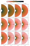 |
Fig. B.1 Logarithmic wind density (in CGS units) displaying the evolution in time for the CAK and LDI models: (top) non-magnetic CAK wind with η⋆ = 0, (middle) strongly confined magnetic CAK wind with η⋆ = 15, and (bottom) strongly confined magnetic LDI wind with η⋆ = 15. The overplotted white lines in the magnetic wind models denote streamlines to illustrate the magnetic field topology. |
References
- Alecian, E., Neiner, C., Wade, G. A., et al. 2015, IAU Symp., 307, 330 [NASA ADS] [Google Scholar]
- Alecian, E., Villebrun, F., Grunhut, J., et al. 2019, EAS Pub. Ser., 82, 345 [NASA ADS] [CrossRef] [EDP Sciences] [Google Scholar]
- Babel, J., & Montmerle, T. 1997, A&A, 323, 121 [NASA ADS] [Google Scholar]
- Bagnulo, S., Wade, G. A., Nazé, Y., et al. 2020, A&A, 635, A163 [NASA ADS] [CrossRef] [EDP Sciences] [Google Scholar]
- Bard, C., & Townsend, R. H. D. 2016, MNRAS, 462, 3672 [NASA ADS] [CrossRef] [Google Scholar]
- Björklund, R., Sundqvist, J. O., Puls, J., & Najarro, F. 2021, A&A, 648, A36 [EDP Sciences] [Google Scholar]
- Blondin, J. M., Kallman, T. R., Fryxell, B. A., & Taam, R. E. 1990, ApJ, 356, 591 [Google Scholar]
- Borra, E. F., Landstreet, J. D., & Mestel, L. 1982, ARA&A, 20, 191 [NASA ADS] [CrossRef] [Google Scholar]
- Carlberg, R. G. 1980, ApJ, 241, 1131 [Google Scholar]
- Castor, J. I., Abbott, D. C., & Klein, R. I. 1975, ApJ, 195, 157 [Google Scholar]
- Colella, P., & Woodward, P. R. 1984, J. Comput. Physi., 54, 174 [NASA ADS] [CrossRef] [Google Scholar]
- Cranmer, S. R., & Owocki, S. P. 1995, ApJ, 440, 308 [NASA ADS] [CrossRef] [Google Scholar]
- Daley-Yates, S., Stevens, I. R., & ud-Doula, A. 2019, MNRAS, 489, 3251 [NASA ADS] [CrossRef] [Google Scholar]
- Das, B., Mondal, S., & Chandra, P. 2020, ApJ, 900, 156 [NASA ADS] [CrossRef] [Google Scholar]
- David-Uraz, A., Owocki, S. P., Wade, G. A., Sundqvist, J. O., & Kee, N. D. 2017, MNRAS, 470, 3672 [NASA ADS] [CrossRef] [Google Scholar]
- David-Uraz, A., Erba, C., Petit, V., et al. 2019a, MNRAS, 483, 2814 [NASA ADS] [CrossRef] [Google Scholar]
- David-Uraz, A., Neiner, C., Sikora, J., et al. 2019b, MNRAS, 487, 304 [NASA ADS] [CrossRef] [Google Scholar]
- Dessart, L., & Owocki, S. P. 2003, A&A, 406, L1 [NASA ADS] [CrossRef] [EDP Sciences] [Google Scholar]
- Dessart, L., & Owocki, S. P. 2005, A&A, 437, 657 [NASA ADS] [CrossRef] [EDP Sciences] [Google Scholar]
- Driessen, F. A., Sundqvist, J. O., & Kee, N. D. 2019a, A&A, 631, A172 [NASA ADS] [CrossRef] [EDP Sciences] [Google Scholar]
- Driessen, F. A., Sundqvist, J. O., & Wade, G. A. 2019b, IAU Symp., 346, 45 [NASA ADS] [Google Scholar]
- Driessen, F. A., Kee, N. D., Sundqvist, J. O., & Owocki, S. P. 2020, MNRAS, 499, 4282 [CrossRef] [Google Scholar]
- Dyda, S., & Proga, D. 2018, MNRAS, 481, 5263 [NASA ADS] [CrossRef] [Google Scholar]
- Eikenberry, S. S., Chojnowski, S. D., Wisniewski, J., et al. 2014, ApJ, 784, L30 [NASA ADS] [CrossRef] [Google Scholar]
- El Mellah, I., & Casse, F. 2017, MNRAS, 467, 2585 [NASA ADS] [Google Scholar]
- Erba, C., David-Uraz, A., Petit, V., et al. 2021, MNRAS, 506, 5373 [NASA ADS] [CrossRef] [Google Scholar]
- Feldmeier, A. 1995, A&A, 299, 523 [NASA ADS] [Google Scholar]
- Feldmeier, A., & Thomas, T. 2017, MNRAS, 469, 3102 [NASA ADS] [CrossRef] [Google Scholar]
- Feldmeier, A., Puls, J., & Pauldrach, A. W. A. 1997, A&A, 322, 878 [NASA ADS] [Google Scholar]
- Feldmeier, A., Oskinova, L., & Hamann, W. R. 2003, A&A, 403, 217 [NASA ADS] [CrossRef] [EDP Sciences] [Google Scholar]
- Fossati, L., Castro, N., Schöller, M., et al. 2015, A&A, 582, A45 [NASA ADS] [CrossRef] [EDP Sciences] [Google Scholar]
- Friend, D. B., & Abbott, D. C. 1986, ApJ, 311, 701 [Google Scholar]
- Friend, D. B., & MacGregor, K. B. 1984, ApJ, 282, 591 [NASA ADS] [CrossRef] [Google Scholar]
- Gagné, M., Oksala, M. E., Cohen, D. H., et al. 2005, ApJ, 628, 986 [CrossRef] [Google Scholar]
- Gayley, K. G. 1995, ApJ, 454, 410 [Google Scholar]
- Georgy, C., Meynet, G., Ekström, S., et al. 2017, A&A, 599, L5 [NASA ADS] [CrossRef] [EDP Sciences] [Google Scholar]
- Gottlieb, S., & Shu, C. W. 1998, Math. Comput., 67, 73 [NASA ADS] [CrossRef] [Google Scholar]
- Grunhut, J. H., Wade, G. A., Neiner, C., et al. 2017, MNRAS, 465, 2432 [NASA ADS] [CrossRef] [Google Scholar]
- Harten, A., Lax, P. D., & Leer, B. v. 1983, SIAM Rev., 25, 35 [CrossRef] [Google Scholar]
- Hawcroft, C., Sana, H., Mahy, L., et al. 2021, A&A, 655, A67 [NASA ADS] [CrossRef] [EDP Sciences] [Google Scholar]
- Hedstrom, G. 1979, J. Comput. Phys., 30, 222 [NASA ADS] [CrossRef] [Google Scholar]
- Hennicker, L., Puls, J., Kee, N. D., & Sundqvist, J. O. 2020, A&A, 633, A16 [NASA ADS] [CrossRef] [EDP Sciences] [Google Scholar]
- Howarth, I. D., & Prinja, R. K. 1989, ApJS, 69, 527 [NASA ADS] [CrossRef] [Google Scholar]
- Howarth, I. D., Walborn, N. R., Lennon, D. J., et al. 2007, MNRAS, 381, 433 [NASA ADS] [CrossRef] [Google Scholar]
- Kaper, L., Henrichs, H. F., Nichols, J. S., et al. 1996, A&AS, 116, 257 [NASA ADS] [CrossRef] [EDP Sciences] [Google Scholar]
- Kee, N. D., Owocki, S., & Sundqvist, J. O. 2016, MNRAS, 458, 2323 [Google Scholar]
- Keppens, R., Teunissen, J., Xia, C., & Porth, O. 2021, Comput. Math. Appl., 81, 316 [Google Scholar]
- Keszthelyi, Z., Meynet, G., Georgy, C., et al. 2019, MNRAS, 485, 5843 [NASA ADS] [CrossRef] [Google Scholar]
- Keszthelyi, Z., Meynet, G., Shultz, M. E., et al. 2020, MNRAS, 493, 518 [NASA ADS] [CrossRef] [Google Scholar]
- Krtička, J., & Feldmeier, A. 2021, A&A, 648, A79 [NASA ADS] [CrossRef] [EDP Sciences] [Google Scholar]
- Küker, M. 2017, Astron. Nachr., 338, 868 [CrossRef] [Google Scholar]
- Lagae, C., Driessen, F. A., Hennicker, L., Kee, N. D., & Sundqvist, J. O. 2021, A&A, 648, A94 [NASA ADS] [CrossRef] [EDP Sciences] [Google Scholar]
- MacGregor, K. B., Hartmann, L., & Raymond, J. C. 1979, ApJ, 231, 514 [Google Scholar]
- Marcolino, W. L. F., Bouret, J. C., Sundqvist, J. O., et al. 2013, MNRAS, 431, 2253 [NASA ADS] [CrossRef] [Google Scholar]
- Martins, F., Hervé, A., Bouret, J. C., et al. 2015a, A&A, 575, A34 [NASA ADS] [CrossRef] [EDP Sciences] [Google Scholar]
- Martins, F., Marcolino, W., Hillier, D. J., Donati, J. F., & Bouret, J. C. 2015b, A&A, 574, A142 [NASA ADS] [CrossRef] [EDP Sciences] [Google Scholar]
- Mestel, L. 1968, MNRAS, 138, 359 [NASA ADS] [CrossRef] [Google Scholar]
- Meynet, G., & Maeder, A. 2000, A&A, 361, 101 [NASA ADS] [Google Scholar]
- Munoz, M. S., Wade, G. A., Nazé, Y., et al. 2020, MNRAS, 492, 1199 [Google Scholar]
- Najarro, F., Hanson, M. M., & Puls, J. 2011, A&A, 535, A32 [NASA ADS] [CrossRef] [EDP Sciences] [Google Scholar]
- Nazé, Y., Ud-Doula, A., Spano, M., et al. 2010, A&A, 520, A59 [NASA ADS] [CrossRef] [EDP Sciences] [Google Scholar]
- Nazé, Y., Bagnulo, S., Petit, V., et al. 2012, MNRAS, 423, 3413 [CrossRef] [Google Scholar]
- Nazé, Y., Petit, V., Rinbrand, M., et al. 2014, ApJS, 215, 10 [CrossRef] [Google Scholar]
- Nazé, Y., Sundqvist, J. O., Fullerton, A. W., et al. 2015, MNRAS, 452, 2641 [CrossRef] [Google Scholar]
- Nazé, Y., ud-Doula, A., & Zhekov, S. A. 2016, ApJ, 831, 138 [CrossRef] [Google Scholar]
- Oksala, M. E., Grunhut, J. H., Kraus, M., et al. 2015, A&A, 578, A112 [NASA ADS] [CrossRef] [EDP Sciences] [Google Scholar]
- Owocki, S. P.,& Puls, J. 1996, ApJ, 462, 894 [Google Scholar]
- Owocki, S. P.,& Rybicki, G. B. 1984, ApJ, 284, 337 [Google Scholar]
- Owocki, S. P.,& Sundqvist, J. O. 2018, MNRAS, 475, 814 [NASA ADS] [CrossRef] [Google Scholar]
- Owocki, S. P.,& ud-Doula, A. 2004, ApJ, 600, 1004 [NASA ADS] [CrossRef] [Google Scholar]
- Owocki, S. P., Castor, J. I., & Rybicki, G. B. 1988, ApJ, 335, 914 [NASA ADS] [CrossRef] [Google Scholar]
- Owocki, S. P., ud-Doula, A., Sundqvist, J. O., et al. 2016, MNRAS, 462, 3830 [NASA ADS] [CrossRef] [Google Scholar]
- Pauldrach, A., Puls, J., & Kudritzki, R. P. 1986, A&A, 164, 86 [NASA ADS] [Google Scholar]
- Petit, V., Owocki, S. P., Wade, G. A., et al. 2013, MNRAS, 429, 398 [NASA ADS] [CrossRef] [Google Scholar]
- Petit, V., Keszthelyi, Z., MacInnis, R., et al. 2017, MNRAS, 466, 1052 [NASA ADS] [CrossRef] [Google Scholar]
- Petit, V., Wade, G. A., Schneider, F. R. N., et al. 2019, MNRAS, 489, 5669 [NASA ADS] [CrossRef] [Google Scholar]
- Poe, C. H., Owocki, S. P., & Castor, J. I. 1990, ApJ, 358, 199 [NASA ADS] [CrossRef] [Google Scholar]
- Powell, K. G., Roe, P. L., Linde, T. J., Gombosi, T. I., & De Zeeuw, D. L. 1999, J. Comput. Phys., 154, 284 [NASA ADS] [CrossRef] [Google Scholar]
- Puls, J., Markova, N., Scuderi, S., et al. 2006, A&A, 454, 625 [NASA ADS] [CrossRef] [EDP Sciences] [Google Scholar]
- Puls, J., Vink,J. S., & Najarro, F. 2008, A&ARv, 16, 209 [Google Scholar]
- Puls, J., Sundqvist, J. O., & Markova, N. 2015, IAU Symp., 307, 25 [Google Scholar]
- Rubio-Díez, M. M., Sundqvist, J. O., Najarro, F., et al. 2021, A&A, in press, https://doi.org/10.1051/0004-6361/202040116 [Google Scholar]
- Runacres, M. C., & Owocki, S. P. 2002, A&A, 381, 1015 [NASA ADS] [CrossRef] [EDP Sciences] [Google Scholar]
- Rybicki, G. B., Owocki, S. P., & Castor, J. I. 1990, ApJ, 349, 274 [NASA ADS] [CrossRef] [Google Scholar]
- Schneider, F. R. N., Ohlmann, S. T., Podsiadlowski, P., et al. 2019, Nature, 574, 211 [Google Scholar]
- Schneider, F. R. N., Ohlmann, S. T., Podsiadlowski, P., et al. 2020, MNRAS, 495, 2796 [NASA ADS] [CrossRef] [Google Scholar]
- Schrøder, S. L., MacLeod, M., Ramirez-Ruiz, E., et al. 2021, ApJ, submitted [arXiv:2107.09675] [Google Scholar]
- Shore, S. N., & Brown, D. N. 1990, ApJ, 365, 665 [NASA ADS] [CrossRef] [Google Scholar]
- Shultz, M. E., Owocki, S., Rivinius, T., et al. 2020, MNRAS, 499, 5379 [NASA ADS] [CrossRef] [Google Scholar]
- Sobolev, V. V. 1960, Moving Envelopes of Stars (Cambridge: Harvard University Press) [Google Scholar]
- Sudnik, N. P., & Henrichs, H. F. 2016, A&A, 594, A56 [NASA ADS] [CrossRef] [EDP Sciences] [Google Scholar]
- Sundqvist, J. O., & Owocki, S. P. 2013, MNRAS, 428, 1837 [Google Scholar]
- Sundqvist, J. O., Owocki, S. P., Cohen, D. H., Leutenegger, M. A., & Townsend, R. H. D. 2012a, MNRAS, 420, 1553 [NASA ADS] [CrossRef] [Google Scholar]
- Sundqvist, J. O., ud-Doula, A., Owocki, S. P., et al. 2012b, MNRAS, 423, L21 [Google Scholar]
- Sundqvist, J. O., Owocki, S. P., & Puls, J. 2018, A&A, 611, A17 [NASA ADS] [CrossRef] [EDP Sciences] [Google Scholar]
- Sundqvist, J. O., Björklund, R., Puls, J., & Najarro, F. 2019, A&A, 632, A126 [NASA ADS] [CrossRef] [EDP Sciences] [Google Scholar]
- Tanaka, T. 1994, J. Comput. Phys., 111, 381 [Google Scholar]
- Thompson, K. W. 1987, J. Comput. Phys., 68, 1 [NASA ADS] [CrossRef] [Google Scholar]
- Townsend, R. H. D., & Owocki, S. P. 2005, MNRAS, 357, 251 [NASA ADS] [CrossRef] [Google Scholar]
- Townsend, R. H. D., Owocki, S. P., & ud-Doula, A. 2007, MNRAS, 382, 139 [NASA ADS] [CrossRef] [Google Scholar]
- Trigilio, C., Leto, P., Umana, G., Leone, F., & Buemi, C. S. 2004, A&A, 418, 593 [NASA ADS] [CrossRef] [EDP Sciences] [Google Scholar]
- ud-Doula, A., & Owocki, S. P. 2002, ApJ, 576, 413 [NASA ADS] [CrossRef] [Google Scholar]
- ud-Doula, A., Townsend, R. H. D., & Owocki, S. P. 2006, ApJ, 640, L191 [NASA ADS] [CrossRef] [Google Scholar]
- ud-Doula, A., Owocki, S. P., & Townsend, R. H. D. 2008, MNRAS, 385, 97 [NASA ADS] [CrossRef] [Google Scholar]
- ud-Doula, A., Owocki, S. P., & Townsend, R. H. D. 2009, MNRAS, 392, 1022 [CrossRef] [Google Scholar]
- ud-Doula, A., Sundqvist, J. O., Owocki, S. P., Petit, V., & Townsend, R. H. D. 2013, MNRAS, 428, 2723 [NASA ADS] [CrossRef] [Google Scholar]
- van der Velden, E. 2020, J. Open Source Softw., 5, 2004 [Google Scholar]
- Vink, J. S., de Koter, A., & Lamers, H. J. G. L. M. 2001, A&A, 369, 574 [NASA ADS] [CrossRef] [EDP Sciences] [Google Scholar]
- Wade, G. A., Grunhut, J., Gräfener, G., et al. 2012, MNRAS, 419, 2459 [NASA ADS] [CrossRef] [Google Scholar]
- Wade, G. A., Barbá, R. H., Grunhut, J., et al. 2015, MNRAS, 447, 2551 [NASA ADS] [CrossRef] [Google Scholar]
- Wade, G. A., Neiner, C., Alecian, E., et al. 2016, MNRAS, 456, 2 [Google Scholar]
- Xia, C., Teunissen, J., El Mellah, I., Chané, E., & Keppens, R. 2018, ApJS, 234, 30 [Google Scholar]
The weight also introduces a fiducial tilt for the (still) radially solved rays to ensure that the wind has not infinitely many critical points which does happen for pure radial rays (CAK).
http://amrvac.org/; version 2.2 (Nov. 2019) in this work.
Namely the number of wave velocities from vr, vr ± aslow, vr ± vAlf, vr ± afast that are greater than zero.
All Tables
All Figures
|
Fig. 1 Logarithmic wind density displaying the evolution in time for our adopted LDI models: (top) non-magnetic wind with η⋆ = 0, (middle) moderately confined wind with η⋆ = 0.15, and (bottom) strongly confined wind with η⋆ = 15. The overplotted white lines in the magnetic wind models represent streamlines to illustrate the magnetic field topology. |
| In the text | |
|
Fig. 2 Lateral averages of statistically computed wind velocity and wind density (dashed lines). Lateral averages are taken in a wedge near the pole (θ = 0−45°, to not have magnetosphere contamination) at simulation termination. Superimposed is a radial cut of wind velocity and density at an arbitrarily chosen colatitude θ within this wedge (solid lines). |
| In the text | |
|
Fig. 3 Radial velocity dispersion laterally averaged over the wedge near the pole (θ = 0− 45°). |
| In the text | |
|
Fig. 4 Statistical contours (from left to right) of wind clumping restricted to a maximum of ten, full wind clumping, radial wind velocity, and poloidal wind velocity for a magnetically confined LDI wind with η⋆ = 15. |
| In the text | |
|
Fig. 5 Modulation of the global mass-loss rate ṀB with wind magnetic confinement |
| In the text | |
|
Fig. 6 Density contrast with respect to the average wind density for the non-magnetic and strongly confined LDI wind model. |
| In the text | |
|
Fig. B.1 Logarithmic wind density (in CGS units) displaying the evolution in time for the CAK and LDI models: (top) non-magnetic CAK wind with η⋆ = 0, (middle) strongly confined magnetic CAK wind with η⋆ = 15, and (bottom) strongly confined magnetic LDI wind with η⋆ = 15. The overplotted white lines in the magnetic wind models denote streamlines to illustrate the magnetic field topology. |
| In the text | |
Current usage metrics show cumulative count of Article Views (full-text article views including HTML views, PDF and ePub downloads, according to the available data) and Abstracts Views on Vision4Press platform.
Data correspond to usage on the plateform after 2015. The current usage metrics is available 48-96 hours after online publication and is updated daily on week days.
Initial download of the metrics may take a while.