| Issue |
A&A
Volume 656, December 2021
|
|
|---|---|---|
| Article Number | A89 | |
| Number of page(s) | 8 | |
| Section | Planets and planetary systems | |
| DOI | https://doi.org/10.1051/0004-6361/202141600 | |
| Published online | 07 December 2021 | |
Photometric survey of 55 near-earth asteroids
1
LESIA, Observatoire de Paris, Université PSL CNRS, Université de Paris, Sorbonne Université,
5 place Jules Janssen,
92195
Meudon,
France
e-mail: This email address is being protected from spambots. You need JavaScript enabled to view it.
2
V. N. Karazin Kharkiv National University,
4 Svobody Sq.,
Kharkiv,
61022, Ukraine
3
IMCCE, Observatoire de Paris, CNRS UMRO 8028, PSL Research University,
77 Av. Denfert Rochereau,
75014
Paris Cedex, France
e-mail: This email address is being protected from spambots. You need JavaScript enabled to view it.
4
Astronomical Institute of the Romanian Academy,
5 Cutitul de Argint, 040557, sector 4,
Bucharest, Romania
5
Institut Universitaire de France (IUF),
1 rue Descartes,
75231
Paris Cedex 05, France
6
Vasile Urseanu Astronomical Observatory,
bd. Lascar Catargiu 21,
010661,
Bucharest, Romania
7
INAF – Osservatorio Astronomico di Roma,
Via Frascati 33,
00078
Monte Porzio Catone, Italy
Received:
21
June
2021
Accepted:
9
September
2021
Abstract
Context. Near-earth objects (NEOs), thanks to their proximity, provide a unique opportunity to investigate asteroids with diameters down to dozens of meters. The study of NEOs is also important because of their potential hazard to the Earth. The investigation of small NEOs is challenging from Earth as they are observable only for a short time following their discovery and can sometimes only be reached again years or decades later.
Aims. We aim to derive the visible colors of NEOs and perform an initial taxonomic classification with a main focus on smaller objects and recent discoveries.
Methods. Photometric observations were performed using the 1.2 m telescope at the Haute-Provence observatory and the 1.0 m telescope at the Pic du Midi observatory in broadband Johnson-Cousins and Sloan photometric systems.
Results. We present new photometric observations for 55 NEOs. Our taxonomic classification shows that almost half (43%) of the objects in our sample are classified as S+Q-complex members, 19% as X-complex, 16% as C-complex, 12% as D-types, and finally 6% and 4% as A- and V-types, respectively. The distribution of the observed objects with H > 19 and H ≤ 19 remains almost the same. However, the majority of the objects in our dataset with D < 500 m belong to the “silicate” group, which is probably a result of an observational bias towards brighter and more accessible objects. “Carbonaceous” objects are predominant among those with a Jovian Tisserand parameter of Tj < 3. These bodies could be dormant or extinct comets. The median values of the absolute magnitude for “carbonaceous” and “silicate” groups are H = 18.10 ± 0.95 and H = 19.50 ± 1.20, whereas the estimated median diameters are D = 1219 ± 729 m and D = 344 ± 226 m, respectively. “Silicate” objects have a much lower median Earth’s minimum orbit intersection distance (MOID) and a somewhat lower orbital inclination in comparison to “carbonaceous” objects. About half of the observed objects are potentially hazardous asteroids and are mostly (almost 65%) represented by “silicate” objects.
Key words: minor planets, asteroids: general / techniques: photometric / surveys
Note to the reader: the email of the second corresponding author M. Birlan has been put back on 10 December 2021.
The NEOROCKS team: E. Dotto, M. Banaszkiewicz, S. Banchi, M. A. Barucci, F. Bernardi, M. Birlan, B. Carry, A. Cellino, J. De Leon, M. Lazzarin, E. Mazzotta Epifani, A. Mediavilla, J. Nomen Torres, D. Perna, E. Perozzi, P. Pravec, C. Snodgrass, C. Teodorescu, S. Anghel, A. Bertolucci, F. Calderini, F. Colas, A. Del Vigna, A. Dell'Oro, A. Di Cecco, L. Dimare, P. Fatka, S. Fornasier, E. Frattin, P. Frosini, M. Fulchignoni, R. Gabryszewski, M. Giardino, A. Giunta, T. Hromakina, J. Huntingford, S. Ieva, J. P. Kotlarz, F. La Forgia, J. Licandro, H. Medeiros, F. Merlin, F. Pinna, G. Polenta, M. Popescu, A. Rozek, P. Scheirich, A. Sergeyev, A. Sonka, G. B. Valsecchi, P. Wajer, A. Zinzi.
© T. Hromakina et al. 2021
 Open Access article, published by EDP Sciences, under the terms of the Creative Commons Attribution License (https://creativecommons.org/licenses/by/4.0), which permits unrestricted use, distribution, and reproduction in any medium, provided the original work is properly cited.
1 Introduction
Near-earth objects (NEOs) are an important source of knowledge regarding the formation and early evolution of the Solar System. Investigation of NEOs can help us to understand the delivery of water and organic material to Earth (e.g., Morbidelli et al. 2000; Marty 2012; Izidoro et al. 2013; Altwegg et al. 2015). Moreover, their richness in water and rare minerals mean that NEOs are of a great interest in regard to potential asteroid mining (Sanchez & McInnes 2013; Calla et al. 2018; Rivkin et al. 2020). Unlike main-belt asteroids, or even more distant small Solar System objects, the proximity of NEOs to the Earth means that even the smallest meter-sized asteroids are accessible to ground-based observations. Moreover, NEOs also create a potential hazard to humanity and life on Earth in general (Perna et al. 2013, 2016). A population of potentially hazardous asteroids (PHAs) is defined by absolute magnitude H ≤ 22, with a diameter D > 140 m assuming an average albedo of 0.14 according to Mainzer et al. (2011), and a minimum orbit intersection distance (MOID) with the Earth of less than 0.05 au (e.g., Perna et al. 2016). The PHAs represent about 8.5% of the total number of discovered NEOs.
All of the known taxonomic classes of asteroids can be found in the NEO population, with about 90% of them distributed among S-, Q-, C-, and X-complex classes (Binzel et al. 2019). Such variety reflects the compositional diversity of the asteroid belt, which is likely the result of mixing due to planetary migration and the resulting dynamical processes (DeMeo & Carry 2014).
The first space missions to NEOs visited silicate bodies (433) Eros (NEAR Shoemaker, Veverka et al. 2000) and (25143) Itokawa (Hayabusa, Saito et al. 2006). More recently, two primitive NEOs were analyzed in detail by sample-return space missions Hayabusa2 (Watanabe et al. 2017) and OSIRIS-REx (Lauretta et al. 2017): (162173) Ryugu and (101955) Bennu, respectively.However, such missions only target individual objects and consistent ground-based surveys are required in order to characterize the entire population of NEOs.
The difficulty in studying the smallest NEOs comes from their faintness, which results in a rather small observability window (Birlan et al. 2015). Therefore, a dedicated rapid-response campaign is needed. The portion of discovered NEOs with known physical properties remains very low: only 20% of the whole population (almost 26 000 objects as of June 2021), and nearly 30% if including only objects larger than 1 km (Perna et al. 2018). The NEOROCKS (NEO Rapid Observation, Characterization, and Key Simulations) project funded by the European Union Horizon 2020 program has been put in place to improve our knowledge of the physical properties of NEOs in the era of a constantly increasing discovery rate of new objects, as well as to address the ever-existing problem of planetary defence.
In this article, we present new photometric observations made in the framework of the NEOROCKS project. Section 2 describes the instrumentation that was used for photometric observations and the data reduction procedure. Section 3 presents the photometry results, taxonomic classification of the observed objects, and statistical analysis of the results. In Sect. 4, we discuss the results, and finally in Sect. 5 we present our conclusions.
2 Observations and data reduction
The observations were performed between March 2020 and April 2021 during several observational runs at the Haute-Provence observatory (OHP, France) and during one run at the Pic du Midi observatory (France). Observations at the OHP were performed using the 1.2 m telescope equipped with a 2048 × 2048 Andor Ikon L 936 CCD camera that has a field-of-view of 13.1′ × 13.1′. A 2 × 2 binning resulted in a pixel scale of 0.77″ pxl−1. Observations at the Pic du Midi observatory were carried out on the 1-m telescope with an iKon-L Andor CCD camera with a 2k × 2k E2V detector (Dumitru et al. 2018). At the OHP, the observations were made using broadband BVRI filters, whereas at the Pic du Midi Sloan griz filters were used.
The targets were selected among visible objects with an apparent brightness of lower than ~19 mag, giving priority to the smallest objects (i.e., those with highest absolute magnitude). At the OHP, each object was observed for about 1 h in all B–V–R–I filters, or only in the V-R-I filters for fainter targets. Most of the objects were observed only once, but some of them were repeatably observed two or three times per run.
Data reduction was carried out following the standard approach, which includes bias subtraction and flat-field correction. Instrumental magnitudes were measured using ASTPHOT software developed by Stefano Mottola (Mottola et al. 1995). Absolute calibration was carried out using field stars from the Pan-STARRS catalog. As the magnitudes in the Pan-STARRS1 catalog are provided in the Sloan photometric system, transformational equations from Kostov & Bonev (2018) were used for data from the OHP. On the contrary, as the majority of the data were obtained using the Johnson-Cousins photometric system, Sloan colors obtained at the Pic du Midi were transformed into the Johnson-Cousins system using equations from Jester et al. (2005).
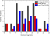 |
Fig. 1 Absolute magnitude distribution of observed NEOs. |
3 Results and data analysis
In total, 55 objects were observed as part of our survey. The orbital elements of the observed objects are presented in Table A.1. Some of the observed targets were too faint, which lead to measured color indexes for 51 NEOs. However, astrometry of these faint objects was nevertheless reported to the Minor Planet Center (MPC). Among objects with measured colors, 27 bodies belong to a group of PHAs and are of particular interest because of their potential hazard to humanity. Figure 1 shows the absolute magnitude distribution in our sample. The absolute magnitude for the majority of objects falls into the H = 17–20 mag range. The distribution for PHAs and nonPHAs in the sample is relatively similar with a slight prevalence of non-PHAs with lower H. The photometry results and observational circumstances are presented in Table 1.
3.1 Taxonomic classification
Based on the measured visible surface colors, we estimated the taxonomic classes of the objects following the classification by DeMeo et al. (2009). The acquired colors were transformed into reflectances relative to the Sun using the solar colors from Holmberg et al. (2006), and then compared with the above-mentioned groups using the M4AST service (Popescu et al. 2012). The estimated taxonomic classes are presented in Table 1. The best-fitting subtype is followed by the complex in which it is included. In the case where the best fit is not clear, we present only the complex the objects falls into. Individual reflectance spectra for each object and the best-fitting mean spectra of the corresponding taxonomic classes are shown in Appendix B. For the statistical analysis, we considered only the main classes, such as S-, C-, and X-complex, and A-, D-, V-types. Although, the difference between S and Q types is the most prominent in the visible region that is covered by our data (DeMeo et al. 2009), we do not distinguish these two classes in order to have better statistics.
Figure 2 shows color–color diagrams for the observed NEOs. The concentration of colors in different areas of the plots follows the typical distribution for the taxonomic classes, indicating the reliability of our classification.
Taxonomy classification was previously carried out for nine objects in our sample, which allowed us to verify our classification using BVRIbroadband photometry. Seven objects (66391, 99942, 152978, 154302, 159402, 163014, and 2004 TP1) were classified into the S-complex group in both the literature and in this work. The object 85989 was classified as K-type in the literature and as D-type inthis work. Finally, NEO 52768 was classified as L or Xk type in the literature and as an X-complex member in this work.
NEOWISE albedo values are available for 13 objects in our sample (Mainzer et al. 2011). We used these values to obtain additional confirmation of our classification. We also used available albedos to classify the objects from the X-complex, which groups together low-albedo primitive P-type objects, moderate-albedo “metallic” M-type objects, and high-albedo enstatite E-type objects following the Tholen taxonomy (Tholen 1984). Six objects that were classified as S-types have moderate albedo, four low-albedo asteroids were classified as D- and C-types, two X-type objects have low albedos that correspond to P-type, and finally one X-type with a high-albedo could be an E-type member. In the interest of a better statistical analysis, we divided the objects based on their surface composition into a “silicate” group that consists of S-complex and A- and V-type objects, and a “carbonaceous” group containing primitive low-albedo asteroids classified as C-complex and D-, and P-types. The rest of the objects, namely X-complex objects with unknown albedo, were grouped into a “miscellaneous” category.
Observational circumstances and photometry results.
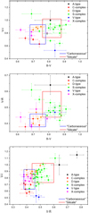 |
Fig. 2 Color–color diagrams showing main taxonomic classes. The boxes represent the 1σ deviation from the mean color values for the group of “silicate” and “carbonaceous” objects. |
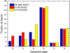 |
Fig. 3 Distribution of the taxonomic classes observed in our survey. |
3.2 Statistical analysis and trends
Based on the taxonomic classification, nearly half of the objects in our sample (22 out of 51) fall into the S-complex, 10 were classified into the X-complex, 8 as D-types, 6 into the C-complex, 3 as A-types, and 2 objects were classified as V-types. The distribution of the taxonomic classes is presented in Fig. 3. In order to look for possible differences in the distribution of the taxonomic classes, we divided our sample into two nearly equal bins considering objects with the absolute magnitude H ≤ 19 and those with H > 19 (H around 19 mag being the median value for our sample). We see almost no difference in the distribution of these two subsamples for our data. For both bins, about 45% of the objects belong to the S-complex and the second-most numerous class is X-complex with about 20% of the objects. The biggest difference occurs for D-type asteroids: their fraction goes from 25% for objects with H ≤ 19 to about 8% for those with H > 19.
As it was already mentioned, albedos and sizes are known for only one-third of the objects in our sample, which is notenough for a statistical analysis. Thus, in order to estimate the sizes of the objects, we used average albedo values for each taxonomic group from Ryan & Woodward (2010). Figure 4 shows the size distribution of our sample. The size estimation for the “miscellaneous” group should be interpreted with care as it is composedof objects with unknown albedo values. There is a prevalence of “silicate” objects in our sample, especially among smaller objects. If we set aside miscellaneous objects because of the ambiguity in the size estimation, the percentage of silicate and “carbonaceous” objects is respectively 80% and 20% for objects with D ≤ 500 m, and 48% and 52% for objects with D > 500 m. Such a distribution is probably caused by an observational bias in our data set.
We compared the estimated diameters with those available in the literature, and for 11 of them the estimation was within the uncertainty of the reported measurements. Two of the objects with size estimations outside of the reported size uncertainties belong to the X-complex group, and the remaining three are classified as C-, D-, and S-type, respectively. The disagreement with the measured values does not exceed 40%.
The Tisserand parameter with respect to Jupiter (Tj) is used to distinguish asteroids with Tj > 3 from cometary objects with T ≤3. The majority of objects fall into the 3 < Tj < 4 range. Objects with Tj < 3 are dominated by carbonaceous objects, which could be extinct or dormant comets. This result is in line with those of Fernández et al. (2001), who found that NEOs with Tj ≤ 3 predominantly have low comet-like albedos.
It was shown by Binzel et al. (2010) that asteroids that fall into the S-complex taxonomic group with lower MOID values tend to have more neutral slopes in the visible region than those with higher MOIDs. Similarly, by analyzing our data we found that the B–R colors of S-complex objects in our sample are correlated with the MOID (Pearson’s coefficient r = 0.86). The trend isshown in Fig. 5. Such a correlation is most probably the result of a refreshing mechanism of the surface at close approaches with the Earth (e.g., DeMeo & Carry 2014).
The median values and the median absolute deviations (MADs) of orbital elements and physical parameters for carbonaceous and silicate objects are shown in Table 2. Silicate bodies in our sample tend to have smaller absolute magnitudes and estimated diameters than carbonaceous objects. The comparison of orbital parameters shows a much smaller median MOID value, and smaller inclinations for the silicate group. On the contrary, other orbital parameters such as e, a, q, and Q are relatively similar for both groups.
Figure 6 shows the value of the Earth’s MOID versus absolute magnitude. Most of the objects with low MOIDs are silicate asteroids; however there are also a few low-albedo objects (C- and D-types) that could be more challenging in terms of mitigation relying on the porosity of the object (Perna et al. 2013; Drube et al. 2015).
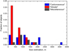 |
Fig. 4 Size distribution of the observed NEOs. |
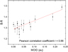 |
Fig. 5 MOID value of S-complex objects in our sample vs. B–R color indexes. The linear regression function is also shown in the plot. |
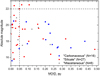 |
Fig. 6 Earth MOID vs. absolute magnitude for different groups of NEOs. The vertical line at MOID = 0.05 au and the horizontal line at H = 22 separate PHAs from the rest of the NEOs. |
4 Discussion
A number of surveys have been dedicated to the study of NEOs (e.g. Binzel et al. 2004, 2019; Devogèle et al. 2019; Ieva et al. 2018, 2020; Perna et al. 2018; Popescu et al. 2019), and as each survey focuses on a certain group of objects (i.e., based on diameters, orbital parameters, etc.), they compliment each other and help us to gain a broader understanding of the NEO population as a whole. The results of our survey are in general agreement with the previous campaigns.
NEOs are dominated by silicate S-type asteroids that originated in the inner part of the main belt. The percentage of S-complex asteroids varies from about 40% (Devogèle et al. 2019), which is closer to our value of 43%, to 60–70% (Ieva et al. 2018; Binzel et al. 2004, 2019). The percentage of X-complex asteroids found in our survey is similar to the value reported by (Devogèle et al. 2019) of about 20%. However, this value is lower in comparison with the percentage found by Binzel et al. (2004, 2019), and Ieva et al. (2020) of about 10%. C-complex members represent 16% in our sample, which is close to the percentage reported by Binzel et al. (2019) and Ieva et al. (2020) and higher than the value in Binzel et al. (2004). D-type asteroids, which represent 12% of our sample, are slightly more abundant than in other surveys for which the amount of D-type NEOs does not exceed ~7% (e.g., Binzel et al. 2004, 2019; Ieva et al. 2020). Finally, the percentage of A- and V-type NEOs remains rather low across all mentioned surveys, but A-type asteroids nevertheless tend to be more abundant among small NEOs (e.g., Perna et al. 2018).
Such variation across the surveys may be caused by the difference in the physical and orbital parameters of the targeted objects, otherwise it could be a result of an observational bias, or both. Each observational campaign is, in one way or another, biased towards brighter and more accessible objects. Additionally, one of the proposed explanations for the dominance of S-type asteroids among NEOs is related to a more efficient migration of these objects from the inner parts of the main belt, compared to C-type asteroids that are more abundant in the outer main belt (Binzel et al. 2004).
According to Binzel et al. (2019), based on sample of more than 1000 NEOs, the distribution of taxonomic classes remains rather stable in the 1–5 km size range. Additionally, the authors found no difference in the distribution of PHAs and nonPHAs. At the same time, a decrease in S + Q complexes and an increase in dark asteroids is found for higher H (Ieva et al. 2020; Devogèle et al. 2019; Perna et al. 2018). The fraction of Q-type asteroids that are believed to be “fresh” or “unweathered” S-types (Binzel et al. 1996) increases due to a combination of effects, such as the YORP-effect, planetary encounters, and seismic shaking (Binzel et al. 2004, 2010; Nesvorný et al. 2005).
Binzel et al. (2004) showed that the most probable source of the X-complex objects is the population of Jupiter-family comets. Therefore, the authors suggested that a large portion of X-complex NEOs should be P-type objects. As already mentioned, our sample has only three X-complex objects with measured albedos (two P-types and one E-type), which does not allow a meaningful analysis in this regard.
The origin of C-complex NEOs is the mid to outer asteroid belt according to Binzel et al. (2004). Spectroscopic and photometric surveys suggest that the percentage of these objects among NEOs does not exceed about 20% of the population (e.g., Ieva et al. 2020; Binzel et al. 2019). However, the actual percentage can be even larger, given that visible and near-infrared surveys are biased towards “bright” populations. Indeed, the NEOWISE survey, which is not affected by such a bias, found the fraction of low-albedo asteroids to be around 25% (Wright et al. 2016). Interestingly, Cg/Cgh types, which show evidence of aqueous altered minerals, are the most rare subtypes of the C-complex (Binzel et al. 2019). The reasons for a lack of such NEOs remain unclear. It could be related to the disappearance of a 0.7 μm absorption band associated with hydrated silicates due to the close proximity of NEOs to the Sun. In our data set, six objects are classified as C-complex, and three of them show the best match with the Cg/Cgh types. However, spectral observations are needed in order to detect the diagnostic absorption band at ~0.7 μm and confirm our taxonomic classification.
Median values and medial absolute deviations (MAD) of orbital elements and physical parameters for carbonaceous and silicate objects.
5 Conclusions
This work contains new photometric observations of 51 NEOs obtained in the framework of NEOROCKS project. As almost half of the objects in our sample belong to the population of PHAs, with these new data we increased the fraction of measured surface colors for this population by about 1%.
The distribution of taxonomic classes among NEOs found in this work is in agreement with the previous surveys. Considering only the main taxonomic classes, we find the following distribution: 43% belong to the S + Q-complex, 19% to the X-complex, 16% to the C-complex, 12% to the D-type, 6% to the A-type, and 4% to the V-types. We did not find a significant difference between the distributions of objects with H ≤ 19 and H > 19. However, considering the estimated equivalent diameters, we note that the majority of the objects in our sample with sizes smaller than 500 m belong to the silicate group, which may be a result of an observational bias.
A taxonomic difference is found in relation to the Jovian Tisserand parameter Tj, where carbonaceous objects make up the majority (57%) of bodies with Tj < 3, suggesting that these objects may be dormant or extinct comets. Moreover, there are some differences in the median physical and orbital parameters for carbonaceous and silicate objects in our sample. Median absolute magnitudes and absolute median deviations for carbonaceous and silicate are H = 18.10 ± 0.95 and H = 19.50 ± 1.20, and the median diameters go from D = 1219 ± 729 m to D = 344 ± 226 m, respectively.Finally, silicate-rich objects in our sample have a lower median value of the Earth’s MOID and slightly lower orbital inclination in comparison to carbonaceous objects.
Acknowledgements
We acknowledge funding from the European Union’s Horizon 2020 research and innovation programme under grant agreement no. 870403. Based in part on observations made at Observatoire de Haute Provence (CNRS), France, and at Pic du Midi observatory, France.
Appendix A Orbital elements of the observed objects
Orbital elements of the observed objects.
Appendix B Individual reflectance spectra of the targets
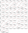 |
Fig. B.1 Individual reflectance spectra of the observed NEOs (red dots) together with the mean spectra of the most likely taxonomic class from DeMeo et al. (2009) (black squares). The spectra are normalized at 0.54 μm. When available, the albedo values and corresponding errors are shown in the plots. |
References
- Altwegg, K., Balsiger, H., Bar-Nun, A., et al. 2015, Science, 347, 1261952 [Google Scholar]
- Binzel, R. P., Bus, S. J., Burbine, T. H., & Sunshine, J. M. 1996, Science, 273, 946 [NASA ADS] [CrossRef] [Google Scholar]
- Binzel, R. P., Rivkin, A. S., Stuart, J. S., et al. 2004, Icarus, 170, 259 [NASA ADS] [CrossRef] [Google Scholar]
- Binzel, R. P., Morbidelli, A., Merouane, S., et al. 2010, Nature, 463, 331 [NASA ADS] [CrossRef] [Google Scholar]
- Binzel, R. P., DeMeo, F. E., Turtelboom, E. V., et al. 2019, Icarus, 324, 41 [Google Scholar]
- Birlan, M., Popescu, M., Nedelcu, D. A., et al. 2015, A&A, 581, A3 [NASA ADS] [CrossRef] [EDP Sciences] [Google Scholar]
- Calla, P., Fries, D., & Welch, C. 2018, ArXiv e-prints, [arXiv:1808.05099] [Google Scholar]
- DeMeo, F. E., & Carry, B. 2014, Nature, 505, 629 [NASA ADS] [CrossRef] [Google Scholar]
- DeMeo, F. E., Binzel, R. P., Slivan, S. M., & Bus, S. J. 2009, Icarus, 202, 160 [Google Scholar]
- Devogèle, M., Moskovitz, N., Thirouin, A., et al. 2019, AJ, 158, 196 [CrossRef] [Google Scholar]
- Drube, L., Harris, A. W., Hoerth, T., et al. 2015, NEOSHIELD – A Global Approach to Near-earth Object Impact Threat Mitigation, 763 [Google Scholar]
- Dumitru, B. A., Birlan, M., Sonka, A., Colas, F., & Nedelcu, D. A. 2018, Astron. Nachr., 339, 198 [NASA ADS] [CrossRef] [Google Scholar]
- Fernández, Y. R., Jewitt, D. C., & Sheppard, S. S. 2001, ApJ, 553, L197 [CrossRef] [Google Scholar]
- Holmberg, J., Flynn, C., & Portinari, L. 2006, MNRAS, 367, 449 [NASA ADS] [CrossRef] [Google Scholar]
- Ieva, S., Dotto, E., Mazzotta Epifani, E., et al. 2018, A&A, 615, A127 [NASA ADS] [CrossRef] [EDP Sciences] [Google Scholar]
- Ieva, S., Dotto, E., Mazzotta Epifani, E., et al. 2020, A&A, 644, A23 [NASA ADS] [CrossRef] [EDP Sciences] [Google Scholar]
- Izidoro, A., de Souza Torres, K., Winter, O. C., & Haghighipour, N. 2013, ApJ, 767, 54 [NASA ADS] [CrossRef] [Google Scholar]
- Jester, S., Schneider, D. P., Richards, G. T., et al. 2005, AJ, 130, 873 [Google Scholar]
- Kostov, A., & Bonev, T. 2018, Bulg. Astron. J., 28, 3 [Google Scholar]
- Lauretta, D. S., Balram-Knutson, S. S., Beshore, E., et al. 2017, Space Sci. Rev., 212, 925 [Google Scholar]
- Mainzer, A., Grav, T., Bauer, J., et al. 2011, ApJ, 743, 156 [NASA ADS] [CrossRef] [Google Scholar]
- Marty, B. 2012, Earth Planet. Sci. Lett., 313, 56 [NASA ADS] [CrossRef] [Google Scholar]
- Morbidelli, A., Chambers, J., Lunine, J. I., et al. 2000, Meteor. Planet. Sci., 35, 1309 [NASA ADS] [CrossRef] [Google Scholar]
- Mottola, S., De Angelis, G., Di Martino, M., et al. 1995, Icarus, 117, 62 [NASA ADS] [CrossRef] [Google Scholar]
- Nesvorný, D., Jedicke, R., Whiteley, R. J., & Ivezić, Ž. 2005, Icarus, 173, 132 [CrossRef] [Google Scholar]
- Perna, D., Barucci, M. A., & Fulchignoni, M. 2013, A&ARv, 21, 65 [CrossRef] [Google Scholar]
- Perna, D., Dotto, E., Ieva, S., et al. 2016, AJ, 151, 11 [Google Scholar]
- Perna, D., Barucci, M. A., Fulchignoni, M., et al. 2018, Planet. Space Sci., 157, 82 [CrossRef] [Google Scholar]
- Popescu, M., Birlan, M., & Nedelcu, D. A. 2012, A&A, 544, A130 [NASA ADS] [CrossRef] [EDP Sciences] [Google Scholar]
- Popescu, M., Vaduvescu, O., de León, J., et al. 2019, A&A, 627, A124 [NASA ADS] [CrossRef] [EDP Sciences] [Google Scholar]
- Rivkin, A. S., Milazzo, M., Venkatesan, A., et al. 2020, ArXiv e-prints, [arXiv:2011.03369] [Google Scholar]
- Ryan, E. L., & Woodward, C. E. 2010, AJ, 140, 933 [NASA ADS] [CrossRef] [Google Scholar]
- Saito, J., Miyamoto, H., Nakamura, R., et al. 2006, Science, 312, 1341 [NASA ADS] [CrossRef] [Google Scholar]
- Sanchez, J.-P., & McInnes, C. R. 2013, Available Asteroid Resources in the Earth’s Neighbourhood, ed. V. Badescu, 439 [Google Scholar]
- Tholen, D. J. 1984, PhD thesis, University of Arizona, Tucson [Google Scholar]
- Veverka, J., Robinson, M., Thomas, P., et al. 2000, Science, 289, 2088 [CrossRef] [Google Scholar]
- Watanabe, S.-i., Tsuda, Y., Yoshikawa, M., et al. 2017, Space Sci. Rev., 208, 3 [Google Scholar]
- Wright, E. L., Mainzer, A., Masiero, J., Grav, T., & Bauer, J. 2016, AJ, 152, 79 [NASA ADS] [CrossRef] [Google Scholar]
All Tables
Median values and medial absolute deviations (MAD) of orbital elements and physical parameters for carbonaceous and silicate objects.
All Figures
|
Fig. 1 Absolute magnitude distribution of observed NEOs. |
| In the text | |
|
Fig. 2 Color–color diagrams showing main taxonomic classes. The boxes represent the 1σ deviation from the mean color values for the group of “silicate” and “carbonaceous” objects. |
| In the text | |
|
Fig. 3 Distribution of the taxonomic classes observed in our survey. |
| In the text | |
|
Fig. 4 Size distribution of the observed NEOs. |
| In the text | |
|
Fig. 5 MOID value of S-complex objects in our sample vs. B–R color indexes. The linear regression function is also shown in the plot. |
| In the text | |
|
Fig. 6 Earth MOID vs. absolute magnitude for different groups of NEOs. The vertical line at MOID = 0.05 au and the horizontal line at H = 22 separate PHAs from the rest of the NEOs. |
| In the text | |
|
Fig. B.1 Individual reflectance spectra of the observed NEOs (red dots) together with the mean spectra of the most likely taxonomic class from DeMeo et al. (2009) (black squares). The spectra are normalized at 0.54 μm. When available, the albedo values and corresponding errors are shown in the plots. |
| In the text | |
Current usage metrics show cumulative count of Article Views (full-text article views including HTML views, PDF and ePub downloads, according to the available data) and Abstracts Views on Vision4Press platform.
Data correspond to usage on the plateform after 2015. The current usage metrics is available 48-96 hours after online publication and is updated daily on week days.
Initial download of the metrics may take a while.