| Issue |
A&A
Volume 656, December 2021
|
|
|---|---|---|
| Article Number | A151 | |
| Number of page(s) | 11 | |
| Section | Stellar structure and evolution | |
| DOI | https://doi.org/10.1051/0004-6361/202140933 | |
| Published online | 16 December 2021 | |
Asteroseismogyrometry of low-mass red giants
I. The SOLA inversion method
1
Korteweg-de Vries Institute for Mathematics, University of Amsterdam, Science Park 105-107, 1098 XG Amsterdam, The Netherlands
e-mail: This email address is being protected from spambots. You need JavaScript enabled to view it.
2
INAF-IAPS Istituto di Astrofisica e Planetologia Spaziali, Via del Fosso del Cavaliere 100, 00133 Roma, Italy
e-mail: This email address is being protected from spambots. You need JavaScript enabled to view it.
3
INAF-Osservatorio Astrofisico di Catania, Via Santa Sofia 78, 95123 Catania, Italy
e-mail: This email address is being protected from spambots. You need JavaScript enabled to view it.
Received:
30
March
2021
Accepted:
27
August
2021
Abstract
Context. During the past 10 years, the unprecedented quality and frequency resolution of asteroseismic data provided by space photometry have revolutionised the study of red-giant stars providing us with the possibility to probe the interior of thousands of these targets.
Aims. Our aim is to present an asteroseismic tool which allows one to determine the total angular momentum of stars, without an a priori inference of their internal rotational profile.
Methods. We adopted the asteroseismic inversion technique developed for the case of the Sun and adapted it to red giants. The method was tested assuming different artificial sets of data, also including modes with harmonic degree l ≥ 2.
Results. We estimate with an accuracy of 14.5% the total angular momentum of the red-giant star KIC 4448777 observed by Kepler during the first four consecutive years of operation.
Conclusions. Our results indicate that the measurement of the total angular momentum of red-giant stars can be determined with a fairly high precision by means of asteroseismology by using a small set of rotational splittings of only dipolar modes; they also show that our method, based on observations of stellar pulsations, provides a powerful mean for testing and modelling the transport of angular momentum in stars.
Key words: asteroseismology / stars: fundamental parameters / stars: individual: KIC 4448777 / stars: oscillations / stars: rotation / stars: interiors
© ESO 2021
1. Introduction
The total angular momentum of a star is a fundamental quantity directly related to its internal structure and rotation rate (e.g. Maeder 2009). Stars lose a significant amount of angular momentum, between their initial formation and the final stages, and the processes transporting it in their interior play a key role in stellar evolution, producing mixing of chemical species and modifying the structure and the chemical gradient between the surface and the core of the star during its life. However, questions related to the transport of angular momentum inside the stars are not yet fully understood: Several mechanisms seem to be active, but they are only approximately modelled or not modelled at all (see e.g. Gough & McIntyre 1998; Spruit 1999, 2002; Charbonnel & Talon 2005; Spada et al. 2010; Maeder & Meynet 2012; Mathis 2013; Zahn 2013; Eggenberger et al. 2017; Aerts et al. 2019).
The study of the stellar total angular momentum is also crucial for a better understanding of the dynamical histories of multi-planet systems and modelling the angular momentum distribution and exchange within a host star and planets. This question, which is quite controversial and widely discussed in literature (e.g. Alves et al. 2010; Paz-Chinchón et al. 2015; Irwin 2015), is currently dealing with several hypotheses including a possible correlation between exoplanetary masses and orbital distances (e.g. Gurumath et al. 2019) as well as a connection between the multiplicity of the systems and their dynamical history (Zinzi & Turrini 2017). In short, the knowledge of the global angular momentum of a star is critical to understand, test, and improve theories able to describe the angular momentum prescriptions in various astrophysical contexts.
The total angular momentum of a star is, however, a quantity inaccessible to direct observations. What one can measure is only the projected surface rotational velocity obtained by stellar spectroscopy, thus it has been evaluated so far just by adopting methods referring to the stellar fundamental parameters and power law relationships, regardless of the real distribution of the mass and angular momentum inside the stellar interior (see, e.g. Irwin 2015).
Over the last decade, the extremely successful observations of stellar pulsations of an unprecedented high quality by the space missions CoRoT (Baglin et al. 2006) and Kepler (Borucki et al. 2010), and even more recently by the current NASA explorer TESS satellite (Ricker et al. 2014) have opened up enormous opportunities and perspectives for improving our knowledge of otherwise hidden stellar interiors and for shedding new light on stellar evolution. In particular, the observation of stellar pulsations has enabled the measurement of the internal rotation in a large sample of stars with different masses and evolutionary stages by using the splittings of the oscillation frequencies caused by rotation in their power spectra. This opportunity is allowing us to put the necessary constraints on stellar angular momentum theories: It has been shown that a strong decrease in the core’s rotation occurs during stellar evolution irrespective of the star’s mass or binarity (Aerts et al. 2019), with values at least two orders of magnitude lower than currently theoretically predicted ones. This is a strong element indicating that one or several mechanisms capable of extracting angular momentum from the core must be at work during stellar evolution (e.g. Marques et al. 2013; Goupil et al. 2013; Cantiello et al. 2014; Ouazzani et al. 2019). Moreover, the efficiency of these, as of yet, unknown angular momentum transport processes appears mass dependent (Eggenberger et al. 2017), although it is not clear if the angular momentum transport increases gradually in efficiency with stellar mass.
Among the asteroseismic targets, the red-giant branch stars (RGB) are of particular interest in this context, showing dense oscillation spectra characterised by the presence of modes with both gravity and acoustic character, known as ‘mixed modes’, able to probe the physical conditions from the inner core to the envelope (e.g. Beck et al. 2012; Deheuvels et al. 2012, 2014; Mosser et al. 2012; Di Mauro et al. 2016). The results thus far have shown in low mass red-giant stars the presence of rapidly rotating helium cores up to 10 times faster than the envelope and shear layers located between the core and the hydrogen burning shell (Di Mauro et al. 2018).
Here, we present a method based on the asteroseismic inversion technique developed by Pijpers (1998), which allows us to compute the total angular momentum of a star by circumventing the need to infer the stellar rotation rate first by the inversion of the observed rotational splittings. This has the great advantage of drastically reducing the number of necessary computational steps and also the systematic errors introduced at each step, ultimately improving the precision and the accuracy of the results.
In the case of the Sun, the total angular momentum deduced by applying the so-called SOLA (subtractive optimally localized averages) inversion technique to 414 acoustic modes by MDI/SOHO, with harmonic degree 1 ≤ l ≤ 250, is  as obtained by Pijpers (1998). More recently Pijpers (2003) demonstrated that it is still possible to obtain an accurate estimate (with an uncertainty of about 3%) of the total angular momentum of the Sun even by inverting a small set of only 14 modes with l = 1. This is not so surprising if we look at the nature of solar acoustic modes, those in which the Sun is observed to oscillate predominantly, and showing amplitudes high enough to be detected at the surface. They, in contrast to gravity modes which in the Sun are trapped in the radiative interior and evanescent in the convection zone, are not very sensitive to the physical structure of the solar core because their energy density is inversely proportional to the sound speed, which is quite large in the solar radiative region. Only low order, low harmonic degree (l ≤ 4) p-modes show energy distributed throughout most of the Sun, providing us a chance of sensing the physical conditions of the solar deepest interior. The result obtained by Pijpers (2003) could pave the way for the SOLA technique to be applied to determine the total angular momentum also in stars other than the Sun, where a small number of modes are detectable in their power spectra.
The aim of this work is to investigate how reliable it could be to estimate the total angular momentum of red-giant stars with a fairly good accuracy even from a small set of data (presumably limited to dipole modes) by applying an adaptation of the SOLA method and taking advantage of the high-precision photometry provided by the most recent space missions. Of course high-precision does not necessarily translate into accuracy, thus we distinguish the statistical error, rising from the uncertainties in the data, from the systematic error arising from the constraints in stellar mass and radius.
In this context the red-giant star KIC 4448777, observed by the Kepler satellite, offers a promising test case. The star, located at the beginning of the ascending red-giant branch, has been observed for more than four years, during the Kepler satellite’s first nominal mission and has been deeply investigated by Di Mauro et al. (2016, 2018). These authors were able to identify 20 rotational splittings of mixed modes over a total of 77 individual observed frequencies and to infer the details of its internal rotational profile. Starting from the resolved rotation rate and the best-fit evolutionary model of the star computed by Di Mauro et al. (2016, 2018), we first derived the value of the total angular momentum by just solving the proper integral equation. Then, we re-computed the global angular momentum of the star by applying the asteroseismic inversion technique proposed by Pijpers (1998, 2003) to the 20 observed splittings and compared the results, thus finally obtaining a test of this method in the case of red-giant stars.
The paper is structured as follows: Sect. 2 provides details on the determination of the total angular momentum in stars and presents the methods for calculating the total angular momentum through the use of asteroseismic data. Section 3 tests the inversion method and shows the results obtained for KIC 4448777. Section 4 discusses the results and draws some conclusions.
2. The total angular momentum
2.1. Basic equations
The total angular momentum of a star is a global fundamental parameter, related to the internal rotation rate and density distribution in the stellar interior through an integral equation:
 (1)
(1)
where x = r/R is the fractional radius, R is the radius of the star, u = cos θ with θ being the co-latitude, Ω(x, u) is the internal rotation rate, and I(x, u) is the scalar moment of inertia, critically dependent on how the stellar mass is distributed inside the star and given by:
 (2)
(2)
where ρ(x) is the density as a function of the fractional radius inside the star.
As a first-order approximation, the angular velocity in the inner regions of a star can be considered almost independent of latitude. As a consequence, integrating Eq. (1) over cos θ, after trivial calculations, produces:
 (3)
(3)
where the total moment of inertia is
 (4)
(4)
The main difficulty in computing this integral in real stars comes from the impossibility of knowing a priori, from classical observations, both the mass distribution inside their interior, namely the dependence of ρ on the fractional radius, and the full radial dependence of the rotation rate profile.
2.2. Computation based on known internal rotational profile
A rough estimate of Jtot in stars has been obtained so far by calculating the moment of inertia over a stellar structure model and adopting the observed projected surface rotation velocity as an approximation of the average internal angular velocity, actually neglecting any dependence on the fractional radius in the interior of the star. Two fundamental questions arise: (i) how representative of the true internal rotation is the surface value adopted (e.g. Benomar et al. 2015; Saio et al. 2015) and (ii) what should the consequence be of the adopted approximation on the accuracy of the results.
In the case of the Sun, in which the deviations from a uniform rotation in the interior are relatively small, the total angular momentum obtained from computations based on the observed surface rotation is Jsurf = 1.63 × 1048 g cm2 s−1 (Cox 2000), a value which is about 14% smaller than that deduced by integrating the internal rotational profile obtained by helioseismic inversion of the MDI/SOHO data J⊙ = (1.96 ± 0.05)×1048 g cm2 s−1 (Di Mauro et al. 1998).
To date, we do not have other direct experiences of these kinds of studies applied to stars more evolved or more massive than the Sun, but we expect even larger discrepancies for the case of distant stars. Nevertheless, we suppose that for any significant study on the dependence of the angular momentum on the stellar mass and age, a high precision should be required.
2.3. The SOLA inversion method
The total angular momentum of a star, as demonstrated by Pijpers (2003), can be determined by the asteroseismic inversion of the following integral equation:
 (5)
(5)
This equation which relates a set of N observed rotational splittings δνi with uncertainties ϵi, for the modes i ≡ (n, l, m) of radial order n, harmonic degree l, and azimuthal order m to the internal angular momentum profile J(x, u), was derived from the application of a standard perturbation theory to an equilibrium stellar structure model, under the hypothesis of slow rotation (Pijpers & Thompson 1994). In fact, the rotation breaks the spherical symmetry of the stellar structure and splits the central frequency of each oscillation mode of harmonic degree l in a multiplet with 2l + 1 components separated by a frequency splitting defined by:
 (6)
(6)
where, for notational convenience, the single index i is used to enumerate the available multiplets nl.
As demonstrated by Pijpers (2003), the 2D expression (Eq. (5)) can be simplified in the following equation:
 (7)
(7)
The individual kernels 𝒦i(x) are a function of the radius only (cf. Pijpers 1997, 2006) and were calculated on the unperturbed eigenfunctions of the modes and other physical quantities of the stellar model which best reproduces all the observational constraints of the star:
![Mathematical equation: $$ \begin{aligned} {\mathcal{K} }_{i}(x)=\rho x^2\left[\xi _{nl}(x)^2 - 2\frac{1}{L}\xi _{nl}(x)\eta _{nl}(x) +\left(1-\frac{1}{L^2}\right)\eta _{nl}(x)^2\right]/{\mathcal{I} }_{nl}, \end{aligned} $$](/articles/aa/full_html/2021/12/aa40933-21/aa40933-21-eq9.gif)
where ξnl(x) and ηnl(x) are the radial and horizontal components of the displacement eigenfunctions of the modes, L2 = l(l + 1), and ![Mathematical equation: $ {\mathcal{I}}_{nl}=\int_0^1\rho \left[\xi_{nl}(x)^2+\eta_{nl}(x)^2\right]{\rm d}x $](/articles/aa/full_html/2021/12/aa40933-21/aa40933-21-eq10.gif) is a normalisation factor which ensures that all kernels integrate to 1 over their domain. This means that the determination of the angular momentum takes the full 2D character of rotation into account, but nevertheless it requires evaluating only 1D integrals. There is also no need to correct for the angle of inclination of the rotation axis with respect to the line of sight.
is a normalisation factor which ensures that all kernels integrate to 1 over their domain. This means that the determination of the angular momentum takes the full 2D character of rotation into account, but nevertheless it requires evaluating only 1D integrals. There is also no need to correct for the angle of inclination of the rotation axis with respect to the line of sight.
The integral Eq. (7) can be solved by applying the SOLA method (Pijpers & Thompson 1992, 1994). The SOLA method is designed to provide a weighted average of a given function by means of a linear combination of all the data, so that:
 (8)
(8)
where ci are the inversion coefficients, and
 (9)
(9)
is the averaging kernel.
When solving the inversion, one should construct a linear combination of kernels, which resembles ‘as closely as possible’ an appropriate chosen target function 𝒯(x). This is possible because compared to the older inversion method by Backus & Gilbert (1970), which is also often referred to as OLA, the SOLA method has the following main advantage: The possibility of choosing any target function that achieves a certain purpose. In the case one wishes to determine a resolved local measurement of the rotation rate, the target function is usually chosen to be a Gaussian, centred on that location. However, while choosing a Gaussian function is a common choice, it is not essential to do so for this method. As demonstrated by Pijpers (2003) when measuring the total angular momentum of a star, the appropriate chosen target function is well represented by the moment of inertia I(x) (see Eqs. (1) and (2)).
As in every inverse method, regularisation is necessary to find an acceptable matching of the averaging kernel to its target function and also to ensure an acceptable small error on the result arising from the propagation of the data errors. In the SOLA method, this regularisation takes the form of balancing, on the one hand, the minimisation of the squared difference of the linear combination of kernels and the target kernel and, on the other hand, minimising the propagated measurement errors. For a given target function 𝒯(x), the expression for the functional ℱ that should be minimised is:
![Mathematical equation: $$ \begin{aligned} \mathcal{F} \equiv \int \limits _0^1\left[\sum \limits _{i}c_{i}{\mathcal{K} }_{i}(x)-{\mathcal{T} }(x)\right]^2 \mathrm{d}x + \mu \sum \limits _{ij} c_{i} E_{ij} c_{j}. \end{aligned} $$](/articles/aa/full_html/2021/12/aa40933-21/aa40933-21-eq13.gif) (10)
(10)
This should be minimised for the linear coefficients ci by adjusting μ, which is an error weighting parameter, while the matrix Eij is the errors’ variance-covariance matrix for the splittings data. While there are cross-validation strategies intended to find an optimal value for μ, in practice some experimentation can be useful or even necessary. When minimising the functional ℱ of Eq. (10) for the coefficients ci, it is usual to enforce that the sum of the coefficients be equal to 1 using a Lagrange multiplier v. Hence, the inversion problem is equivalent to solving the following set of linear equations (see Pijpers & Thompson 1994):
 (11)
(11)
where W is the symmetric (N + 1)×(N + 1) mode cross-correlation matrix whose elements are  and v is the vector which includes the cross-correlation eigenvalues of the kernels with the target function 𝒯(x):
 (12)
(12)
The solutions of Eq. (11) are the inversion coefficients ci collected in the vector c, obtained by inverting the matrix W only once.
3. Asteroseismogyrometry of the red-giant KIC 4448777
3.1. Computation by integrating the angular velocity profile
KIC 4448777, located at the beginning of the ascending red-giant branch, is a solar-like star, where oscillations stochastically excited by turbulent convection, as in the Sun, have allowed Di Mauro et al. (2016, 2018) to fully characterise its structure. Having exhausted its central hydrogen supply, it has a degenerate helium core surrounded by a hydrogen shell that is still burning. Table 1 reports the main characteristics of the star. In particular, the effective temperature, the gravity, and iron abundances [Fe/H] were obtained from spectroscopic campaigns. The large separation Δν, reported in Table 1, was calculated by the linear fit over the asymptotic relation for the observed radial mode frequencies (see Di Mauro et al. 2018, for more details). The asteroseismic mass M = (1.12 ± 0.09) M⊙ and radius R = (4.13 ± 0.11) R⊙ were directly obtained by the asteroseismic scaling laws based only on the spectroscopic atmospheric parameters and the asteroseismic measurements of Δν and νmax, the observed large separation and frequency of the maximum amplitude power respectively.
Main observed and theoretical parameters for KIC 4448777.
Table 1 also shows all the theoretical parameters of the best model, including the luminosity L, the age, the location of the base of the convective region rcz/R, and the extent of the He core rHe/R of the stellar reference model selected in Di Mauro et al. (2016, 2018) as the result of the best-fitting procedure between KIC 4448777 and hundreds of evolutionary models built in order to match all the observational spectroscopic and seismic constraints simultaneously, including all the 77 individual observed frequencies with harmonic degree l = 0, 1, 2, 3. This is part of a standard and well developed procedure for the entire asteroseismic analysis, which ensures that the chosen reference model provides the closest possible description of the real star. In particular, this selection is necessary for the application of any inversion method which requires linearisation around a reference model close enough to the actual star in order to provide reliable results. The procedure of selection was largely discussed in Di Mauro et al. (2016, 2018).
The star has been observed by the Kepler satellite for more than four years, during its first nominal mission and its internal rotation has been successfully determined by means of asteroseismic inversion (Di Mauro et al. 2018). The detection of 20 rotational splittings of mixed modes allowed the authors to reconstruct the angular velocity profile into the interior of the star in detail, showing that the helium core rotates almost rigidly about 6 times faster than the convective envelope, while part of the hydrogen shell seems to rotate at a constant velocity, about 1.15 times lower than the He core.
The total angular momentum of KIC 4448777 obtained by integrating Eq. (3) and using Ω(x) determined by the inversion of the rotational splittings in Di Mauro et al. (2018) is  and the moment of inertia integrating Eq. (4) is Itot = 1.85 × 1055 g cm2. The large error in Jtot reflects the low spatial resolution with which the angular velocity can be determined in the regions relevant for the determination of the angular momentum, as shown in Fig. 1 which reports the radial dependence of the angular momentum computed for the best-fit model of KIC 4448777 and the radial profile of the rotation rate as inferred in Di Mauro et al. (2018). The contribution to the total angular momentum inside the star mainly comes from the layers of the convective envelope between r = 0.2 R and r = 0.9 R (see Fig. 1), where the uncertainties in the angular velocity are higher, while the remaining part of the star is almost unimportant, despite the high velocity rate in the inner regions.
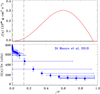 |
Fig. 1. Upper panel: radial profile of the angular momentum inside the best-fit model of KIC 4448777 according to the definition of Eq. (3). Lower panel: radial profile of the angular velocity as obtained by inversion of rotational splittings in Di Mauro et al. (2018). Dashed lines show the base of the convective zone rcz = 0.1448 R and the external edge of the He core rHe = 0.0074 R. |
This result is mostly determined by the radial distribution of the moment of inertia inside the star, as can be seen in Fig. 2, where the moment of inertia I(x) calculated for our best-fit model of KIC 4448777 and, for comparison, for model S of the Sun (Christensen-Dalsgaard et al. 1996) are shown. By simply considering that the total moment of inertia can be split into two integrals calculated over the two adjacent regions, the convective envelope and the radiative layer,
 (13)
(13)
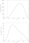 |
Fig. 2. Radial profile of the moment of inertia inside the best-fit model of KIC 4448777 (top panel) and – for comparison – inside model S of Christensen-Dalsgaard et al. (1996) for the Sun (low panel). The location of the base of the convective zone is shown by dashed lines. |
we can try to roughly understand which region is mostly contributing to the moment of inertia as a solar-type star evolves. The respective values of Icz and Irad given in Table 2 show that, at odds with the Sun, only the convective envelope is significantly contributing to the total moment of inertia of KIC 4448777: The core and the H-burning shell have a very high density, but they are strongly confined in a fraction of the stellar radius that is too small, while the upper layers in the red giants are far too tenuous to be able to supply substantial contributions. We show in the next sections that the direct asteroseismic method suggested by Pijpers (2003) provides a more powerful tool to determine accurate estimates of the total angular momentum also in stars other than the Sun, without the need to solve a priori the inner rotational profile.
Moment of inertia inside the convective envelope Icz and in the radiative region Irad calculated for our best-fit model of KIC 4448777 and for a solar model.
3.2. Testing the SOLA inversion procedure
In order to test the potential of the SOLA procedure for the case of red giants, we carried out a ‘hare-and-hounds’ exercise, in which the hare is represented by the total angular momentum calculated for the best-fit model of KIC 4448777 summarised in Table 1 and assuming a simple fictitious rotational profile given by:
This rotational profile, by solving Eq. (3), produces an angular momentum J(1) = 1.49 × 1048 g cm2 s−1.
Using a forward seismological approach, as described in Di Mauro et al. (2016), we computed a set of 20 artificial rotational splittings for l = 1 from the above step-like rotational law. To get a realistic estimate of the capabilities of the inversion, this synthetic set of data comprises the same modes observed for KIC 4448777 and for each rotational splitting we adopted the same error of 15 nHz, which is the average of the errors of the observed data (between 0.5 nHz ≤ ϵ ≤ 30 nHz).
The hounds are the values of angular momentum  obtained by the attempts at inversion of the set of artificial splittings by varying the trade-off parameter μ in order to determine the closest value to J(1). As explained in Sect. 2, because of the ill-conditioned nature of the inversion problem, we should apply a regularisation procedure by varying the trade-off parameter μ in order to choose a good compromise between the uncertainty of the solution and the mismatch between the averaging kernel K(x) and the target kernel 𝒯(x) given by:
![Mathematical equation: $$ \begin{aligned} \chi ^2=\int _0^1 \left[\sum \limits _{i} c_{i}{\mathcal{K} }_{i}(x) -{\mathcal{T} }(x)\right]^2\,\mathrm{d}x. \end{aligned} $$](/articles/aa/full_html/2021/12/aa40933-21/aa40933-21-eq21.gif) (14)
(14)
The choice of the value of μ, which strongly depends on the magnitude of the errors in the data and on the oscillation modes determines the trade-off necessary between the accuracy and precision of the solution. By lowering the trade-off parameter, it is possible to obtain averaging kernels closer to the target kernels, which in other words means a lower χ2 value, but this decreases the precision with which the solution is determined, since the weight of the errors increases. Thus, we should choose, among all the possible solutions, the one obtained for a value of μ which provides an optimal compromise between a low χ2 and a small error in the result.
By varying the trade-off parameter between 100 ≤ μ ≤ 3000, for μ = 140, we obtained the solution  characterised by χ2 = 12, which represents the best agreement with J(1). This is nicely shown in the trade-off diagram of Fig. 3 (left panel), where the variation of the total angular momentum
  is plotted against various values of μ, while the values of χ2 are shown on the ordinate axis on the right.
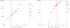 |
Fig. 3. Hare and hound attempts for a set of synthetic data including the same modes as those observed for KIC 4448777. Inversion solutions (red diamonds) are plotted as function of the trade-off parameter μ and the relative values of χ2. Left panel: results for a set of splittings with errors ϵi = 15 nHz. Right panel: results for the same synthetic set assuming real observed errors as in Di Mauro et al. (2018). The theoretical value J(1) = 1.49 × 1048 g cm2 s−1, which should be matched by the inversion procedure, is shown by the blue dotted line. |
In order to evaluate the weight of the errors affecting the observed splittings, in a second ‘hare-and-hounds’ exercise we inverted the same set of artificial splittings, but we adopted real errors as those affecting the observed data set of KIC 4448777 (Di Mauro et al. 2018). By varying the trade-off parameter between 100 ≤ μ ≤ 8000, for μ = 3800, we obtained the value of  , which for the inversion of this set represents the closest value and hence the best agreement with J(1), characterised by χ2 = 31. The regularisation procedure can be visualised in Fig. 3 (right panel), which shows the obtained inversion solutions
  and the relative χ2 as functions of different values of the trade-off parameter μ.
Figure 4 compares averaging and target kernels for these tests. In practice, as shown in Pijpers & Thompson (1994), it is impossible to reproduce perfectly the target kernel as a consequence of the fact that the problem is ill-posed: The set of data includes a finite number of observational constraints, the solution is not unique, and, in addition, it is highly sensitive to noise. Nevertheless, as already explained in Sect. 3.1, we should not be bothered by the difference below r = 0.2 R and above R = 0.9 R, because these regions do not substantially contribute to the measurement of the angular momentum in the star (see Sect. 2). It is interesting to point out that χ2 gets closer to 1 if we ignore the mismatch for r < 0.05 R. As it can be seen by comparing the two panels of Fig. 3 with the two panels of Fig. 4, the better precision of the data produces a better precision in the inversion result, but real and smaller errors in the data reflect a worse agreement between averaging and target kernels, that is, higher χ2.
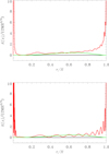 |
Fig. 4. Averaging resolving kernel (in red) plotted in comparison with the target kernel (in green) for the inversion of a set of 20 artificial splittings with l = 1 calculated for the best-fit model of the red giant KIC 4448777. Top panel: inversion of artificial data with errors equal to 15 nHz and a trade-off parameter μ = 140. Bottom panel: inversion of artificial data with real errors and μ = 3800. |
The overall good agreement found in these exercises shows that in the case of red giants, in which the dramatic structural changes due to evolution have determined the onset of mixed modes, the total angular momentum can be estimated fairly well by using sets of rotational splittings of only dipolar modes. The reason for that is the peculiar behaviour of mixed modes. Those of them characterised by low inertia mainly propagate in low-density layers (the acoustic cavity) of the star and behave mostly as p modes, while those characterised by a rather high inertia mainly propagate in high-density regions (the gravity-wave cavity) and behave as g modes.
However the radial distance between the acoustic and gravity cavities, well separated in main sequence solar-like oscillators, becomes progressively smaller as the star evolves, allowing g modes to couple with p modes at some stage. In red giants, several g modes can couple with a single p mode of a similar frequency and the same harmonic degree, leading to a plethora of mixed modes per acoustic radial order with gravity characteristics in the deep interior, acoustic behaviour in the outer layers, and amplitudes that are enhanced enough to be detectable at the surface. Coupling is most effective for dipole modes, while it is weaker for quadrupole and higher harmonic degree modes because of the larger evanescent zone between the two cavities. In addition, as a consequence of the smaller amplitudes at the stellar surface, modes with l > 1 are harder to detect.
A close look at the behaviour of the individual kernels of some dipolar modes, which are computed for our best-fit model of KIC 4448777 and plotted in Fig. 5, further clarify this point. Dipolar modes characterised by different frequencies and energies propagate in different way in the internal stellar structure, from the core to the surface. As a consequence, in order to adequately probe the interior of a red giant, it is sufficient to handle a set of modes with a different gravity-acoustic character and energy (see, e.g. Di Mauro et al. 2011).
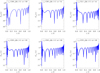 |
Fig. 5. Individual kernels as calculated for the best-fit model of KIC 4448777 for six dipolar modes detected in the star. In each panel, the corresponding frequency ν, the harmonic degree l, and the radial order n are indicated. |
3.3. Improving the angular momentum determination
The results obtained raise the natural question of whether the accuracy and the precision in the computation of the angular momentum should be further improved by increasing the number of rotational splittings in the inverted data set. To answer this question, we computed artificial splittings with harmonic degree l ≥ 2 and frequencies ranging in the observed interval of significant power for KIC 4448777, 160 μHz ≤ ν ≤ 280 μHz. An error of 15 nHz has been assumed for all the modes. The plots reported in Fig. 6, obtained for the individual kernels of modes with increasing l = 1 − 6, show that the acoustic cavity moves progressively towards the surface as the value of the harmonic degree increases, causing modes with a higher degree to probe layers closer and closer to the surface more efficiently. At the same time for l > 2, the mixed modes in the interval of detected frequencies appear to show a predominant gravity nature with kernels characterised by a large amplitude in the core as l increases, becoming less adequate to be used as seismic probes of the acoustic cavity.
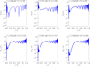 |
Fig. 6. Individual kernels as calculated for the best-fit model of KIC 4448777 for 6 modes with increasing value of the harmonic degree. In each panel the corresponding theoretical frequency ν, the harmonic degree l and the radial order n are indicated. |
The comparison of the results obtained by inverting several sets of data including mixed modes with harmonic degree l ≥ 2 provide us the answer to the original question: In red giants, the angular momentum can be estimated with an agreement between the averaging kernel and the target kernel that can only be subtly improved by considering an increasing number of splittings in the inverted data set, even using a large set of data. In parallel, the precision of the result gets worse. For example, the result of the hare and hounds exercise for a set of data which includes 448 modes with harmonic degree 1 ≤ l ≤ 6 produced  for μ = 435.5 and a χ2 = 6. This result, compared to the one obtained by inverting only 20 rotational splittings, clearly shows that no major improvement was gained by using such a large set of mixed modes; the uncertainty gets even worse, while the accuracy represented by a lower χ2 slightly improves. Figure 7 shows the comparison between the averaging and target kernels for the inversion of the large set of 448 artificial splittings.
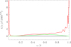 |
Fig. 7. Averaging resolving kernel (in red) and target kernel (in green) for the inversion of a set of 448 artificial splittings calculated on the best-fit model of KIC 4448777 with l = 1 − 6, errors ϵi = 15 nHz and a trade-off parameter μ = 435.5. |
It may appear counter-intuitive that adding more data, and therefore incorporating more kernels in the inversion, does not lead to improvements. The reason can be found in the information contained in the available kernels and can be understood by considering the vector and matrix notation of the inversion problem given in Eq. (11). The eigenfunctions of the oscillation modes, from which the kernels were constructed through Eq. (9), of course form an orthogonal complete base set. One might infer from this that each new measured rotational splitting included in the set should add new independent information. However, the eigenfunctions Wij of the (N + 1)×(N + 1) matrix W do not appear to be orthogonal, in fact some of them are associated to the same eigenvalue, leading to an effective reduction of the independent information which one can derive from the data set. Hence, one way of quantifying the information content in the available data set is to consider the eigenvalues spectrum vi of the cross correlation matrix of the rotational kernels of the set obtained after the inversion (Eq. (11)).
The eigenvalues indicate how many independent solutions the system of linear equations has and hence they give information about how ill-conditioned the problem is. The eigenvalues are scalars and are usually sorted in descending order, providing information on the reduction of the components of the new subspace for the matrix W:
 (15)
(15)
The left panel of Fig. 8, obtained for the adopted set of 448 artificial data, shows the resulting eigenvalues vi plotted in order of increasing index, simply as a function of the position in the matrix from 1 to 449. The sequence is characterised by several plateaus, levels of small decline, or no growth, indicating that the data generate the same eigenvalues. If two (or more) eigenvalues are identical, the system of linear equations is degenerate so that there are two (or more) different eigenvectors, or eigensolutions since each eigenvector corresponds to a function, which can be combined into any linear combination and also satisfy the eigensolution properties. If two eigenvalues are not perfectly identical, but very close in value, as is the case here, then the corresponding eigensolution functions are normally also very similar in oscillatory character, that is, with a very similar wavelength, but slightly different places for their maxima and minima. The right panel of Fig. 8 reports the degeneracy of the eigenvalues for the adopted set, showing that out of 448 modes, only about 18 are contributing and adding information to the inversion, while the others are adding only noise to the inversion result. This is not surprising and it was already pointed out for the case of the Sun by Pijpers & Thompson (1994), who, when applying the SOLA inversion technique to estimate the solar internal rotation, found that only 66 out of the 834 observed modes included in the data set were really useful for the inversion.
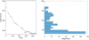 |
Fig. 8. Left panel: eigenvalues of the inversion matrix (Eq. (11)), plotted as a function of the increasing position index, as obtained for a set of 448 artificial splittings with l = 1 − 6. Different colours indicate similar solutions obtained for the system of linear equations inverted. Right panel: histogram of the degeneracy of the eigenvalues, i.e. the number of times a similar number appears in the vector of eigenvalues. |
It is well known that the degeneracy of the eigenvalues is always related to some spatial symmetry of the system. In the present case, this is due to the nature of the mixed modes and the way in which these modes probe the interior of red-giant stars, as discussed above. According to what we have learnt from the Sun, we would expect a different conclusion if the inverted data set could also include pure p or g modes, which unfortunately are not excited in red-giant stars. The implication is that each extra measured rotational splitting does not add completely independent information to the set.
Since any real measured or even artificial data set consists of a finite number of frequency splittings, the dimension of the functional space spanned by the corresponding eigenfunctions is also limited. Due to the degeneracy, the dimension of the function space spanned by the kernels is even smaller, and it barely increases as the number of available splittings increases. Especially when all the available modes are mixed modes, with a very short spatial wavelength in the core, adding further modes in the inversion algorithm produces an averaging kernel which crosses the target kernel very often, so that at those locations the inversion appears successful, but at the same time the averaging kernel has much larger deviations from its target at other values of r/R. For any given data set, this behaviour can only be suppressed by penalising large values for the linear coefficients, that is setting the regularisation parameter μ to very high values. In other words, the take-home lesson here is that diversity of the modes represented by the data is more important than merely having a large quantity of modes.
3.4. Angular momentum by applying the SOLA method
Since the properties of the inversion depend, for a given stellar model, on the errors in the rotational splittings and the modes included in the data set, the trade-off parameter μ = 3800 found with the hare and hounds test in Sect. 3.2 can be adopted for the inversion of the observed set of data. The result obtained by applying the SOLA method to the red-giant star KIC 4448777 indicates a value of the total angular momentum  , a value which is in good agreement with Jtot obtained in Sect. 3.1, but much better constrained. The percentage error ΔJstat/J⋆ = 0.5% only corresponds to the statistical uncertainty coming from the errors propagation in the inversion procedure and is only related to the observed frequency splitting uncertainties.
In order to get a more realistic estimate of the angular momentum, we need to consider the contribution to the global error coming from the accuracy with which the selected stellar model best fits the observations of the star. It is demonstrated by Deheuvels et al. (2014) that no significant difference is found in the inversion results for the internal rotation by using different stellar models, as long as these models are consistent with each other to first order, which means that they are able to match both seismic and non-seismic parameters within the errors. Di Mauro et al. (2016) show that two selected best-fit models, chosen on the basis of the χ2 criterion, produce similar rotational inversion results. The good agreement of the results has also been confirmed by applying different independent methods (i.e. the method proposed by Goupil et al. 2013 and a least-squares fit to the observed rotational splittings).
Reese (2015) explains that some discrepancy due to the use of different models arise from the fact that different models might have oscillation modes with different inertia because of possible different extents of the acoustic and gravity cavities. In the case of red giants, the regions above the core are mostly sounded by modes with a mixed g–p character, whose identification is more crucial than modes with a dominant p or g behaviour, respectively, and they are better trapped in the convective region and in the inner core (see, e.g. Mosser et al. 2011, 2012). Fortunately, mixed modes of different inertia have very different damping times and profiles in the observed oscillation spectrum (see, e.g. Mosser et al. 2018). Thus, the analysis of the observations (see, e.g. Corsaro & De Ridder 2014) can provide essential information on the gravity or acoustic nature of each detected oscillation mode and the best-fit stellar model is chosen by using the nature of each mode, not only the oscillation frequencies as additional constrains. Furthermore, Schunker et al. (2016) explored the sensitivity of the inversion procedure to different stellar models and they conclude that for Sun-like stars with moderate radial differential rotation gradients, the inversions are insensitive to uncertainties in the stellar models.
In order to quantify the dependence of the result on the assumed stellar structure model, we can simply consider that the angular momentum depends on the moment of inertia – roughly given by I ∝ MR2 – that is on the distribution of the mass inside the stellar models and also on the total mass and radius of the star. Considering that the accuracy level of asteroseismic estimates by using only the average seismic parameters for KIC 4448777 as calculated in Di Mauro et al. (2016) and shown in Table 1 is ΔM/M = 8% for the stellar mass and ΔR/R = 3% for the stellar radius, we determined that in order to take the uncertainty in model computations into account, it is necessary to consider an additional relative systematic error of about ΔJsyst/J⋆ = 14%, corresponding to an uncertainty of ΔJsyst = 0.55 × 1048 g cm2 s−1.
We can conclude that the total angular momentum of KIC 4448777 can be evaluated by applying the SOLA asteroseismic technique and it is:
 (16)
(16)
with a total relative uncertainty of ΔJ/J⋆ = 14.5%. This result is an enormous improvement with respect to the method of integrating Eq. (3), based on the known internal rotational profile, despite the relatively small set of rotational splittings, covering a limited range in l, available for the inversion.
Finally, we tested the above estimate of the total uncertainty by adopting a different evolutionary model fitting, within the errors, both seismic and non-seismic observations of KIC 4448777 well, but with a lower goodness of the chi-square test as described in Di Mauro et al. (2018). The second-best model is characterised by the following parameters: M = 1.02 M⊙, Teff = 4800 K, R = 3.94 R⊙, and log g = 3.26 dex. Once a different best trade-off parameter for this model was selected by performing a new hare and hounds test, for μ = 2160, we obtained a value of
 (17)
(17)
and χ2 = 29. The reported uncertainty includes the statistical error ΔJstat = 0.02 coming from the inversion procedure, which is merely related to the observed frequency splitting uncertainties, and the systematic error ΔJsyst = 0.41 arising from uncertainty in the stellar mass and radius of the adopted model. We can conclude that the results  and
and  obtained by using the two different best-fitting models are in agreement within the errors and hence we can confirm that the procedure is model-independent within the limits described above.
4. Discussion and conclusion
This paper has demonstrated that the total angular momentum of red-giant stars can be well and properly determined through the SOLA asteroseismic inversion technique. More interestingly, this holds even if a relatively limited set of data, including rotational splittings of only dipolar modes, is available.
The usual route is to first determine an average internal angular velocity or, ‘as best as possible’, a spatially resolved rotation rate and then reintegrate that after multiplying by the moment of inertia calculated for the adopted ‘best’ evolutionary model of the star. This route has unfortunate error propagation properties, with the result that the uncertainty in the angular momentum, due to the measurement errors of the data, becomes quite large.
Here we have analysed the inference of the total angular momentum of KIC 4448777, a red-giant star of stellar mass M = (1.12 ± 0.09) M⊙, in which observations performed by the space mission Kepler have allowed us to detect 20 rotational splittings of oscillation frequencies of harmonic degree l = 1. By using an appropriate target kernel within the SOLA formalism, described here, the angular momentum of this star has been determined from the inversion of splittings directly, taking the full 2D character of the internal rotational profile into account. We find that the SOLA inversion procedure is characterised by good error propagation properties. This allowed us to obtain a total angular momentum ![Mathematical equation: $ \overline{J_\star}\pm(\Delta J_{\mathrm{stat}} + \Delta J_{\mathrm{syst}}) = [3.90 \pm(0.02+0.55)] \times 10^{48}\,\mathrm{g\,cm^2\,s^{-1}} $](/articles/aa/full_html/2021/12/aa40933-21/aa40933-21-eq33.gif) for our star, where the total uncertainty includes the statistical error rising from the data and the systematic error due to the accuracy in the mass and radius of the star. For KIC 4448777, which is characterised by very precise observational data, it is just this last source of error which dominates the total uncertainty. This is generally an issue for any star other than the Sun.
for our star, where the total uncertainty includes the statistical error rising from the data and the systematic error due to the accuracy in the mass and radius of the star. For KIC 4448777, which is characterised by very precise observational data, it is just this last source of error which dominates the total uncertainty. This is generally an issue for any star other than the Sun.
Moreover, it should not be a surprise that, even if asteroseismic inversions (Di Mauro et al. 2016, 2018) have produced a radial profile of the angular velocity of KIC 4448777 characterised by low resolution in the convective envelope (see low panel of Fig. 1), the global angular momentum results are not affected by such large errors. In fact, the SOLA inversion method in the present work has not been applied to search for localised solutions along the stellar radius, but to determine a global parameter.
In addition, it has been demonstrated that in order to determine the total angular momentum of red-giant stars with a good precision and accuracy, it is sufficient to use data sets which include rotational splittings of only dipolar modes as those already obtained for several targets by the photometric space missions and a model which best fits the seismic and non-seismic observations of the star. The contribution to the analysis of splittings of high-harmonic degree modes does not seem to improve the precision of the inversion since we have demonstrated that the diversity of the oscillation trapping character, which translates into modes with different inertia, is more important than the employment of just a large number of modes. It is clear that a large data set would contribute to better constrain the best-fit model necessary for the inversion procedure and then improve the accuracy of the result.
In the present paper, we did not explore how changes to the input stellar models might affect the inversion results. Nevertheless, the precision of the actual asteroseismic data sets demands that the sources of systematic errors have to be addressed. Hence, it will be worthwhile in the future to carry out a systematic study devoted to investigate how the choice of the best-fit model might impact the inversion of angular momentum, as it was done previously for the determination of the angular velocity. This can be done by employing different evolutionary codes with different input physics regarding diffusion, core overshoot, and rotation, even though the largest source of error in all the asteroseismic studies unfortunately still arises from modelling the near-surface layers (Jørgensen et al. 2021, and references therein). This procedure will provide a smaller systematic error than we currently estimate.
In the near future, we plan to extend this technique to the large sample of solar-like stars for which rotational splittings of dipolar oscillation modes have been successfully detected by Kepler/K2. In particular it will be interesting to study the evolution of the stellar total angular momentum from the main sequence to later stages by selecting observed stars with similar stellar masses, but in different evolutionary phases. This will allow to understand the dependence of the angular momentum on the age of the star and possibly to estimate the amount of angular momentum transferred from the core to the envelope during the evolution in order to balance the rotational velocity.
Moreover, we will try to understand if main sequence solar-like stars with detectable rotational splittings (Benomar et al. 2015), and to some extent also subgiants, might represent better subjects in this context. In these stars, the target kernel and the achievable averaging kernel might show a better match due to the use of observed data sets, which mainly include acoustic modes with a low harmonic degree trapped in the regions relevant for the evaluation of their total angular momentum. Furthermore, we plan to apply this technique even to intermediate- or high-mass stars, in which tens of rotational splittings of g and p modes have already been detected (Aerts et al. 2019).
We believe that our tool based on a data-driven approach, in which very accurate space mission observations act as a test bench for theoretical simulations and models, will help to understand fundamental processes governing the variation of the internal rotation of stars with time, such as the core-envelope coupling or the angular momentum loss from the surface. The estimate of the total angular momentum of a star, incorporated as an essential ingredient or as a boundary condition into rotating stellar evolutionary codes, will produce the needed advancement of the theory of angular momentum transport in stellar interiors.
The application limit of this technique might be the difficulty in measuring rotational splittings of oscillation modes with an amplitude that is too low to be detected with a sufficient accuracy or hidden in a forest of multiple modes of oscillations in different kinds of stars. However, the space missions NASA/TESS (Ricker et al. 2014), launched in April 2018, and ESA/PLATO (Rauer et al. 2016), which is to be launched in the 2026, have the potential to enable us to detect rotational splittings and hence to infer the total angular momentum in a large sample of stars, including high-mass and metal-poor stars in binaries and clusters.
Acknowledgments
The authors thank very much the anonymous referee for his/her useful suggestions and comments, which gave the opportunity to greatly improve the manuscript.
References
- Aerts, C., Mathis, S., & Rogers, T. M. 2019, ARA&A, 57, 35 [Google Scholar]
- Alves, S., Do Nascimento, J. D., Jr., & de Medeiros, J. R. 2010, MNRAS, 408, 1770 [NASA ADS] [CrossRef] [Google Scholar]
- Backus, G., & Gilbert, F. 1970, Philos. Trans. R. Soc. London Ser. A, 266, 123 [NASA ADS] [CrossRef] [Google Scholar]
- Baglin, A., Auvergne, M., Boisnard, L., et al. 2006, 36th COSPAR Scientific Assembly, 36, 3749 [Google Scholar]
- Beck, P. G., Montalban, J., Kallinger, T., et al. 2012, Nature, 481, 55 [Google Scholar]
- Benomar, O., Takata, M., Shibahashi, H., Ceillier, T., & García, R. A. 2015, MNRAS, 452, 2654 [Google Scholar]
- Borucki, W. J., Koch, D., Basri, G., et al. 2010, Science, 327, 977 [Google Scholar]
- Cantiello, M., Mankovich, C., Bildsten, L., Christensen-Dalsgaard, J., & Paxton, B. 2014, ApJ, 788, 93 [Google Scholar]
- Charbonnel, C., & Talon, S. 2005, Science, 309, 2189 [Google Scholar]
- Christensen-Dalsgaard, J., Dappen, W., Ajukov, S. V., et al. 1996, Science, 272, 1286 [Google Scholar]
- Corsaro, E., & De Ridder, J. 2014, A&A, 571, A71 [NASA ADS] [CrossRef] [EDP Sciences] [Google Scholar]
- Cox, A. N. 2000, Allen’s Astrophysical Quantities (New York: Springer-Verlag) [Google Scholar]
- Deheuvels, S., García, R. A., Chaplin, W. J., et al. 2012, ApJ, 756, 19 [Google Scholar]
- Deheuvels, S., Doğan, G., Goupil, M. J., et al. 2014, A&A, 564, A27 [NASA ADS] [CrossRef] [EDP Sciences] [Google Scholar]
- Di Mauro, M. P., Dziembowski, W. A., & Paternó, L. 1998, in Structure and Dynamics of the Interior of the Sun and Sun-like Stars, ed. S. Korzennik, ESA Spec. Publ., 418, 759 [NASA ADS] [Google Scholar]
- Di Mauro, M. P., Cardini, D., Catanzaro, G., et al. 2011, MNRAS, 415, 3783 [NASA ADS] [CrossRef] [Google Scholar]
- Di Mauro, M. P., Ventura, R., Cardini, D., et al. 2016, ApJ, 817, 65 [NASA ADS] [CrossRef] [Google Scholar]
- Di Mauro, M. P., Ventura, R., Corsaro, E., & Lustosa De Moura, B. 2018, ApJ, 862, 9 [Google Scholar]
- Eggenberger, P., Lagarde, N., Miglio, A., et al. 2017, A&A, 599, A18 [NASA ADS] [CrossRef] [EDP Sciences] [Google Scholar]
- Gough, D. O., & McIntyre, M. E. 1998, Nature, 394, 755 [Google Scholar]
- Goupil, M. J., Mosser, B., Marques, J. P., et al. 2013, A&A, 549, A75 [NASA ADS] [CrossRef] [EDP Sciences] [Google Scholar]
- Gurumath, S. R., Hiremath, K. M., & Ramasubramanian, V. 2019, PASP, 131, 014401 [NASA ADS] [CrossRef] [Google Scholar]
- Irwin, S. A. 2015, PhD Thesis, Florida Institute of Technology, USA [Google Scholar]
- Jørgensen, A. C. S., Montalbán, J., Angelou, G. C., et al. 2021, MNRAS, 500, 4277 [Google Scholar]
- Maeder, A. 2009, Physics, Formation and Evolution of Rotating Stars (Berlin, Heidelberg: Springer-Verlag) [Google Scholar]
- Maeder, A., & Meynet, G. 2012, Rev. Mod. Phys., 84, 25 [Google Scholar]
- Marques, J. P., Goupil, M. J., Lebreton, Y., et al. 2013, A&A, 549, A74 [NASA ADS] [CrossRef] [EDP Sciences] [Google Scholar]
- Mathis, S. 2013, in Transport Processes in Stellar Interiors, eds. M. Goupil, K. Belkacem, C. Neiner, F. Lignières, & J. J. Green (Berlin, Heidelberg: Springer-Verlag), 865, 23 [Google Scholar]
- Mosser, B., Barban, C., Montalbán, J., et al. 2011, A&A, 532, A86 [NASA ADS] [CrossRef] [EDP Sciences] [Google Scholar]
- Mosser, B., Goupil, M. J., Belkacem, K., et al. 2012, A&A, 540, A143 [NASA ADS] [CrossRef] [EDP Sciences] [Google Scholar]
- Mosser, B., Gehan, C., Belkacem, K., et al. 2018, A&A, 618, A109 [NASA ADS] [CrossRef] [EDP Sciences] [Google Scholar]
- Ouazzani, R. M., Marques, J. P., Goupil, M. J., et al. 2019, A&A, 626, A121 [NASA ADS] [CrossRef] [EDP Sciences] [Google Scholar]
- Paz-Chinchón, F., Leão, I. C., Bravo, J. P., et al. 2015, ApJ, 803, 69 [CrossRef] [Google Scholar]
- Pijpers, F. P. 1997, A&A, 326, 1235 [NASA ADS] [Google Scholar]
- Pijpers, F. P. 1998, MNRAS, 297, L76 [NASA ADS] [CrossRef] [Google Scholar]
- Pijpers, F. P. 2003, A&A, 402, 683 [NASA ADS] [CrossRef] [EDP Sciences] [Google Scholar]
- Pijpers, F. P. 2006, Methods in Helio- and Asteroseismology (London: Imperial College Press) [CrossRef] [Google Scholar]
- Pijpers, F. P., & Thompson, M. J. 1992, A&A, 262, L33 [NASA ADS] [Google Scholar]
- Pijpers, F. P., & Thompson, M. J. 1994, A&A, 281, 231 [NASA ADS] [Google Scholar]
- Rauer, H., Aerts, C., Cabrera, J., & PLATO Team 2016, Astron. Nachr., 337, 961 [Google Scholar]
- Reese, D. R. 2015, A&A, 578, A37 [NASA ADS] [CrossRef] [EDP Sciences] [Google Scholar]
- Ricker, G. R., Winn, J. N., Vanderspek, R., et al. 2014, SPIE Conf. Ser., 9143, 914320 [Google Scholar]
- Saio, H., Kurtz, D. W., Takata, M., et al. 2015, MNRAS, 447, 3264 [Google Scholar]
- Schunker, H., Schou, J., & Ball, W. H. 2016, A&A, 586, A24 [NASA ADS] [CrossRef] [EDP Sciences] [Google Scholar]
- Spada, F., Lanzafame, A. C., & Lanza, A. F. 2010, MNRAS, 404, 641 [NASA ADS] [CrossRef] [Google Scholar]
- Spruit, H. C. 1999, A&A, 349, 189 [NASA ADS] [Google Scholar]
- Spruit, H. C. 2002, A&A, 381, 923 [CrossRef] [EDP Sciences] [Google Scholar]
- Zahn, J. P. 2013, in EAS Publications Series, eds. G. Alecian, Y. Lebreton, O. Richard, & G. Vauclair, 63, 245 [CrossRef] [EDP Sciences] [Google Scholar]
- Zinzi, A., & Turrini, D. 2017, A&A, 605, L4 [NASA ADS] [CrossRef] [EDP Sciences] [Google Scholar]
All Tables
Moment of inertia inside the convective envelope Icz and in the radiative region Irad calculated for our best-fit model of KIC 4448777 and for a solar model.
All Figures
|
Fig. 1. Upper panel: radial profile of the angular momentum inside the best-fit model of KIC 4448777 according to the definition of Eq. (3). Lower panel: radial profile of the angular velocity as obtained by inversion of rotational splittings in Di Mauro et al. (2018). Dashed lines show the base of the convective zone rcz = 0.1448 R and the external edge of the He core rHe = 0.0074 R. |
| In the text | |
|
Fig. 2. Radial profile of the moment of inertia inside the best-fit model of KIC 4448777 (top panel) and – for comparison – inside model S of Christensen-Dalsgaard et al. (1996) for the Sun (low panel). The location of the base of the convective zone is shown by dashed lines. |
| In the text | |
|
Fig. 3. Hare and hound attempts for a set of synthetic data including the same modes as those observed for KIC 4448777. Inversion solutions (red diamonds) are plotted as function of the trade-off parameter μ and the relative values of χ2. Left panel: results for a set of splittings with errors ϵi = 15 nHz. Right panel: results for the same synthetic set assuming real observed errors as in Di Mauro et al. (2018). The theoretical value J(1) = 1.49 × 1048 g cm2 s−1, which should be matched by the inversion procedure, is shown by the blue dotted line. |
| In the text | |
|
Fig. 4. Averaging resolving kernel (in red) plotted in comparison with the target kernel (in green) for the inversion of a set of 20 artificial splittings with l = 1 calculated for the best-fit model of the red giant KIC 4448777. Top panel: inversion of artificial data with errors equal to 15 nHz and a trade-off parameter μ = 140. Bottom panel: inversion of artificial data with real errors and μ = 3800. |
| In the text | |
|
Fig. 5. Individual kernels as calculated for the best-fit model of KIC 4448777 for six dipolar modes detected in the star. In each panel, the corresponding frequency ν, the harmonic degree l, and the radial order n are indicated. |
| In the text | |
|
Fig. 6. Individual kernels as calculated for the best-fit model of KIC 4448777 for 6 modes with increasing value of the harmonic degree. In each panel the corresponding theoretical frequency ν, the harmonic degree l and the radial order n are indicated. |
| In the text | |
|
Fig. 7. Averaging resolving kernel (in red) and target kernel (in green) for the inversion of a set of 448 artificial splittings calculated on the best-fit model of KIC 4448777 with l = 1 − 6, errors ϵi = 15 nHz and a trade-off parameter μ = 435.5. |
| In the text | |
|
Fig. 8. Left panel: eigenvalues of the inversion matrix (Eq. (11)), plotted as a function of the increasing position index, as obtained for a set of 448 artificial splittings with l = 1 − 6. Different colours indicate similar solutions obtained for the system of linear equations inverted. Right panel: histogram of the degeneracy of the eigenvalues, i.e. the number of times a similar number appears in the vector of eigenvalues. |
| In the text | |
Current usage metrics show cumulative count of Article Views (full-text article views including HTML views, PDF and ePub downloads, according to the available data) and Abstracts Views on Vision4Press platform.
Data correspond to usage on the plateform after 2015. The current usage metrics is available 48-96 hours after online publication and is updated daily on week days.
Initial download of the metrics may take a while.