| Issue |
A&A
Volume 655, November 2021
|
|
|---|---|---|
| Article Number | A69 | |
| Number of page(s) | 12 | |
| Section | Planets and planetary systems | |
| DOI | https://doi.org/10.1051/0004-6361/202141941 | |
| Published online | 19 November 2021 | |
Measuring titanium isotope ratios in exoplanet atmospheres
1
Leiden Observatory, Leiden University,
Postbus 9513,
2300 RA
Leiden,
The Netherlands
e-mail: This email address is being protected from spambots. You need JavaScript enabled to view it.
2
Max-Planck-Institut für Astronomie,
Königstuhl 17,
69117
Heidelberg,
Germany
Received:
3
August
2021
Accepted:
30
September
2021
Abstract
Context. Measurements of relative isotope abundances can provide unique insights into the formation and evolution histories of celestial bodies, tracing various radiative, chemical, nuclear, and physical processes. In this regard, the five stable isotopes of titanium are particularly interesting. They are used to study the early history of the Solar System, and their different nucleosynthetic origins help constrain Galactic chemical models. Additionally, titanium’s minor isotopes are relatively abundant compared to those of other elements, making them more accessible for challenging observations, such as those of exoplanet atmospheres.
Aims. We aim to assess the feasibility of performing titanium isotope measurements in exoplanet atmospheres. Specifically, we are interested in understanding whether processing techniques used for high-resolution spectroscopy, which remove continuum information about the planet spectrum, affect the derived isotope ratios. We also want to estimate the signal-to-noise requirements for future observations.
Methods. We used an archival high-dispersion CARMENES spectrum of the M-dwarf GJ 1002 as a proxy for an exoplanet observed at very high signal-to-noise. Both a narrow (7045–7090 Å) and wide (7045–7500 Å) wavelength region were defined for which spectral retrievals were performed using petitRADTRANS models, resulting in isotope ratios and uncertainties. These retrievals were repeated on the spectrum with its continuum removed to mimic typical high-dispersion exoplanet observations. The CARMENES spectrum was subsequently degraded by adding varying levels of Gaussian noise to estimate the signal-to-noise requirements for future exoplanet atmospheric observations.
Results. The relative abundances of all minor Ti isotopes are found to be slightly enhanced compared to terrestrial values. A loss of continuum information from broadband filtering of the stellar spectrum has little effect on the isotope ratios. For the wide wavelength range, a spectrum with a signal-to-noise of 5 is required to determine the isotope ratios with relative errors ≲10%. Super Jupiters at large angular separations from their host star are the most accessible exoplanets, requiring about an hour of observing time on 8-meter-class telescopes, and less than a minute of observing time with the future Extremely Large Telescope.
Key words: planets and satellites: gaseous planets / planets and satellites: atmospheres / planets and satellites: composition / stars: abundances / stars: individual: GJ 1002 / techniques: spectroscopic
© ESO 2021
1 Introduction
The relative abundances of isotopes in a given environment are determined by various radiative, chemical, nuclear, and physical processes that occurred throughout its history. Understanding the effects of these processes on the isotope ratios can therefore trace the formation and evolution of astronomical objects. For instance, preferential Jeans escape of protium (1H) and bombardment by deuterium-rich comets are invoked to explain the enhanced deuterium-to-hydrogen (D/H) ratio1 of Earth’s ocean water compared to the protosolar nebula (e.g., Genda & Ikoma 2008; Hartogh et al. 2011). Recently, work has begun to plan and perform isotope measurements in exoplanet atmospheres. For instance, Lincowski et al. (2019) and Morley et al. (2019) discuss the feasibility of determining hydrogen and oxygen isotope ratios in exoplanet atmospheres using the upcoming James Webb Space Telescope. Mollière & Snellen (2019) studied the efficacy of determining isotope ratios using ground-based high-resolution ( ) spectroscopy, and conclude that while D/H measurements will only be possible with the future Extremely Large Telescope, current 8-m-class telescopes should be capable of determining carbon isotope ratios in exoplanets. Indeed, Zhang et al. (2021) measured an isotope ratio in an exoplanet for the first time, finding a super-terrestrial 13C/12C value for the young super-Jupiter TYC 8998 b using medium-resolution (
 ) integral field spectroscopy. Since this planet orbits well beyond the CO snowline, they suggest its enhancement in 13C could be due to accretion of ices enriched in 13C by isotope fractionation processes. This may mark the beginning of using isotope ratios to probe formation histories of planets beyond our Solar System.
Titanium has five stable isotopes – 46Ti, 47Ti, 48Ti, 49Ti, and 50Ti – with telluricrelative abundances of 8.25%, 7.44%, 73.72%, 5.41%, and 5.18% (Meija et al. 2016). With about 25% of its atoms approximately equally partitioned among the minor (less abundant) isotopes, Ti compares favorably to hydrogen(Wood et al. 2004; Linsky et al. 2006; Altwegg et al. 2015, and the references therein), carbon (Milam et al. 2005; Asplund et al. 2009; Meija et al. 2016), and oxygen (Ayres et al. 2013, and the references therein; Romano et al. 2017, and the references therein), whose minor isotopes have relative abundances ≲2% in the Solar System and local interstellar medium. The isotopes of titanium have different nucleosynthetic origins, with oxygen and silicon burning in massive stars thought to be the main source of 46Ti and 47Ti, while 48Ti, 49Ti, and 50Ti are thought to be mostly produced in type Ia and/or type II supernovae (Hughes et al. 2008, and the references therein). It is therefore expected that stars that formed in different environments may exhibit variations in Ti isotope ratios of a factor ~2 or more (Hughes et al. 2008). Indeed, observational studies targeting TiO isotopologue2 features in K- and M-dwarfs have determined relative deviations of tens of percent in Ti isotope ratios compared to terrestrial values (Wyckoff & Wehinger 1972; Lambert & Luck 1977; Clegg et al. 1979; Chavez & Lambert 2009; Pavlenko et al. 2020). Such measurements have, in turn, been used to constrain Galactic chemical models (e.g., Hughes et al. 2008).
Interestingly, relative abundances of Ti isotopes are also used to study the early evolution of the Solar System. For instance, variations in isotope ratios across different populations of meteorites and other Solar System bodies are used to study (in)homogeneity and thermal processing in the solar protoplanetary disk (e.g., Leya et al. 2008; Trinquier et al. 2009). Conversely, the similarity in telluric and lunar Ti isotope ratios places constraints on Moon formation theories (Zhang et al. 2012). We note, however, that the relative variations reported in the Solar System are ≲0.1%, which is orders of magnitude smaller than those found in stellar populations.
Both close-orbiting and young gas giants can have sufficiently high temperatures (T ≳ 1500–2000 K) to allow gaseous TiO to persist in their atmospheres (e.g., Hubeny et al. 2003; Fortney et al. 2008; Spiegel et al. 2009; Gandhi & Madhusudhan 2019), possibly enabling similar Ti isotope analyses of these objects. Indeed, there is increasing evidence for TiO in hot Jupiters from transmission and dayside emission spectra (e.g., Nugroho et al. 2017; Serindag et al. 2021; Cont et al. 2021; Chen et al. 2021). The youngest super Jupiters, which are still hot from their formation, are also expected to show TiO features, similar to brown dwarfs and M-dwarf stars. In fact, TiO band heads are clearly visible in the medium-resolution MUSE optical spectrum of the young, wide-orbiting super-Jupiter GQ Lupi b (Stolker et al., in prep.).
In this paper, we use an archival high-dispersion CARMENES spectrum of the M-dwarf GJ 1002 as a proxy for a gas-giant exoplanet observed at extremely high signal-to-noise, and assess the feasibility of performing titanium isotope measurements in exoplanet atmospheres. We investigate how the derived isotope ratios are impacted by different wavelength coverage and a loss of continuum information, which is a common effect of the processing techniques for high-resolution spectroscopy of exoplanet atmospheres. We also estimate what spectral signal-to-noise ratios (S/Ns) are needed to perform such analyses for exoplanets, along with the corresponding exposure times for current 8-m-class telescopes and the future Extremely Large Telescope. In Sect. 2, we describe the high-resolution stellar spectrum we use in this work. We present the high-resolution TiO model spectra in Sect. 3 and outline our fitting methodology in Sect. 4. We present and discuss the results of our analyses in Sects. 5 and 6, before summarizing our work in Sect. 7.
2 High-resolution TiO spectral data
2.1 CARMENES spectrum of GJ 1002
We use a single high-resolution archival3 spectrum of the M5.5V (Walker 1983) star GJ 1002 taken on 18 November 2016 using the CARMENES spectrograph on the 3.5-m Calar Alto Telescope. CARMENES (Quirrenbach et al. 2014) consists of two echelle spectrographs in the visible and near-infrared wavelength regime. The archival observation is a 1238-s exposure in the visual channel, covering 5200–10 500 Å at a resolving power of  (≈3 km s−1). The automated CARACAL pipeline (Caballero et al. 2016; Zechmeister et al. 2018) performs the initial data processing including bias correction, order extraction, and wavelength calibration. The archival pipeline product contains the topocentric wavelengths, fluxes, and errors for the 61 orders of the visual channel.
We isolated wavelengths 7000–7600 Å from nine orders and removed all pixels (0.02%) with nonfinite flux values. To mitigate the influence of telluric contamination, we also removed all wavelength bins (9%) with a telluric transmission value ≤0.98, based on the ESO SkyCalc model (Noll et al. 2012; Jones et al. 2013) with a precipitable water vapor of 2.5 mm. We subsequently shifted the spectrum to the stellar rest frame and divided the flux and error values by the mean flux level in the spectral range 7045–7050 Å preceding the red-degraded γ-system (0,0) band head of TiO at 7054 Å. This wavelength range is similar to those used as continuum levels in previous studies fitting high-resolution stellar TiO features (Clegg et al. 1979; Valenti et al. 1998; Chavez & Lambert 2009). The top left panel of Fig. 1 shows the normalized spectrum (hereafter, unfiltered spectrum) over the wavelength range 7045–7500 Å.
To mimic the standard treatment of high-resolution spectra in exoplanet atmosphere analyses, we performed a high-pass filter which results in the loss of continuum information. For each wavelength bin, we subtracted the mean flux value in a boxcar with a full width of 0.60 Å (≈ 25 km s−1). Since the pixel spacing is nonuniform in both wavelength and velocity space, we only filtered a given pixel if its boxcar contains more than half of the expected number of pixels based on the average wavelength sampling. This results in 2% of the pixels being excluded. This broadband-filtered spectrum on 7045–7500 Å is shown in the bottom left panel of Fig. 1.
2.2 Choice of wavelength range for TiO fitting
Most of the previous studies that used TiO to determine stellar Ti isotope ratios used the wavelength range ~7050–7100 Å, which contains strong features of the TiO γ-system (0,0) bands. Lambert & Mallia (1972), Wyckoff & Wehinger (1972), Lambert & Luck (1977), and Chavez & Lambert (2009) all chose a range with a relatively low line density between the γ(0,0) band heads at 7054 Å and 7089 Å. Clegg et al. (1979) used a similar spectral range, but only for stars with a spectral type earlier than M4. For M4 stars and later, they instead analyzed the regions around the γ-system (0,1) band at 7589 Å and δ-system (0,0) band around 8900 Å, which are less saturated.
More recently, Pavlenko et al. (2020) compared the suitability of various spectral ranges in the optical and near-infrared for TiO isotopologue analysis, and they argue that the spectral region 7580–7594 Å, including the γ(0,1) band head at 7589 Å, is preferable to the commonly used spectral window encompassing the γ(0,0) band. Specifically, they note that while the γ(0,0) band head at 7054 Å is a blend of features from all five TiO isotopologues, the γ(0,1) band heads of 49TiO and 50TiO are blue-shifted out of the stronger, red-degraded 48TiO band head at 7589 Å. Further, they note that the stellar flux for late-type stars is higher at these redder wavelengths than at 7054 Å. This is also expected to be the case for exoplanets. However, a major drawback of using the region surrounding the γ(0,1) band at 7589 Å is the presence of the strong telluric O2 A band at 7590 Å. As Pavlenko et al. (2020) point out, the separation between the telluric and TiO band heads – and thus the level of telluric contamination of the TiO band – depends on the relative velocity between the target and telescope.
Since the primary objective of this work is to determine the feasibility of deriving accurate Ti isotope ratios from TiO features in the spectra of gas-giant exoplanets, we opt to entirely avoid analyzing spectral regions near the strong O2 A band. Instead, similar to the majority of previous studies, we performed spectral fitting using the range 7045–7090 Å (hereafter, narrow range), shown for the unfiltered and broadband-filtered cases in the top right and bottom right panels of Fig. 1. To investigate whether including more, albeit weaker, TiO features affects the spectral fitting results for GJ 1002 or enables more accurate results for noise-degraded cases, we also analyze the spectral range 7045–7500 Å (hereafter, wide range). The top left and bottom left panels of Fig. 1 show the unfiltered and broadband-filtered spectrum, respectively, over this wide wavelength range. For comparison, the narrow range is highlighted in blue.
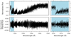 |
Fig. 1 Top left panel: unfiltered CARMENES spectrum of GJ 1002 over the wide wavelength range 7045–7500 Å. The narrow wavelength range 7045–7090 Å is indicated by the blue shading. Top right panel: same as top left panel, but plotting only the narrow wavelength range for clarity. Bottom left panel: broadband-filtered CARMENES spectrum of GJ 1002 over the wide wavelength range. Bottom right panel: same as bottom left panel, but for the narrow wavelength range. |
3 High-resolution TiO spectral models
We used the radiative transfer code petitRADTRANS (Mollière et al. 2019) to model the TiO spectrum of GJ 1002. While originally developed to study exoplanets, the high-resolution emission spectrum functionality of petitRADTRANS is also appropriate for modeling stellar spectra. We modeled the atmosphere of GJ 1002 in 70 layers from 105 to 10−6 bar assuming a constant, solar mean molecular weight of 2.33. We linearly interpolated the temperature–pressure (T–P) profiles of the MARCS plane-parallel standard-composition stellar model atmospheres grid (Gustafsson et al. 2008) to the parameters of GJ 1002. Specifically, we adopted a microturbulent velocity vturb = 2 km s−1 and fixed the remaining stellar parameters based on their literature values from Rajpurohit et al. (2018): Teff = 3100 K, log g = +5.5, and [M ∕H] = +0.20. Since the MARCS models do not span a pressure range comparable to our atmospheric model, we subsequently extrapolated the T–P profile based on linear fits in log T– logP space. To reflect the maximum temperature for which we calculated TiO opacities, we imposed a temperature upper limit of 4000 K.
We only included spectroscopic contributions from the five main isotopologues4 of TiO, as these dominate the M-dwarf optical spectrum. We utilized the recently released ExoMol TOTO line list to calculate TiO opacities. Compared to other commonly used TiO line lists, ExoMol TOTO reproduces the TiO features in high-resolution M-dwarf spectra better for both the main (48TiO) and minor isotopologues due to the inclusion of more accurate experimental energy levels in the line list calculations (McKemmish et al. 2019; Pavlenko et al. 2020). We used the method outlined in Appendix A of Mollière et al. (2015) to calculate TiO opacities up to 4000 K on a high-resolution wavelength grid (λ∕dλ = 106). For all TiO isotopologues, we assumed a constant volume mixing ratio (VMR) at each pressure layer in our model atmosphere.
To facilitate a better fit, we performed similar processing steps on the petitRADTRANS models as we used on the CARMENES data. We broadened the models to the CARMENES resolving power and subsequently interpolated them onto the wavelength sampling of the data. We then normalized the model spectra to their mean flux value in the range7045–7050 Å. If we were fitting the broadband-filtered CARMENES spectrum, we also performed a boxcar filtering identical to that described in Sect. 2.1. As an example, Fig. A.1 plots an unfiltered model (dashed black line) over a limited wavelength range, calculated using TiO isotopologue abundances retrieved for GJ 1002 (see Sects. 4 and 5). Also shown are the flux contributions of the individual TiO isotopologues (solid lines), demonstrating their influence on the composite model spectrum.
4 Fitting TiO isotopologue abundances
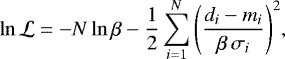
We used the EMCEE implementation (Foreman-Mackey et al. 2013) of the Goodman & Weare (2010) affine-invariant Markov chain Monte Carlo (MCMC) ensemble sampler to directly fit the processed CARMENES spectrum (Sect. 2.1) using the similarly processed petitRADTRANS models (Sect. 3). Following the methods presented by Brogi & Line (2019) and Gibson et al. (2020), we adopted a log-likelihood function of the form
 (1)
(1)
where N is the number of pixels, di and mi are the data and model flux values for the ith pixel, σi is the CARMENES error of the ith pixel, and β is a wavelength-invariant scaling factor for the uncertainties. The purpose of the latter term is to allow for the possibility that the CARMENES errors are underestimated and to attempt to account for systematic uncertainties in our models.
Our model consists of six fitted parameters: β and the  for each TiO isotopologue5. We adopted uniform priors: [1, 100] for β, [−10, − 6] for
  , and [−13, − 6] for each minor isotopologue’s
  . The choice of bounds for the TiO abundances allows for ratios relative to the main isotopologue 48TiO of [10−3, 1], which is essentially zero to unity. Whilewe did not fit for Teff, log g, [M ∕H], vturb, and the mean molecular weight (see Sect. 3), we did perform additional retrievals to estimate the impact that uncertainties in these parameters have on the TiO results (see Sect. 6.1).
For each fit, we performed two MCMC runs in sequence. For the first, we initialized 50 walkers uniformly within the bounds of the prior for each fitted parameter, and we ran the sampler for 500 steps, corresponding to 25 000 model evaluations. We then initialized 50 walkers in a Gaussian ball around the best-fitting set of parameters from the first run and evolved the sampler again for 1000 steps (50 000 model evaluations). We visually inspected and removed the section of the second run preceding convergence. The resulting clipped, converged chain is the set of posterior samples used in our analysis.
5 Results
5.1 Ti isotope ratios for the M-dwarf GJ 1002
Using the framework presented in Sect. 4, we performed multiple retrievals of the TiO isotopologue abundances in the M-dwarf GJ 1002 to assess the impact of different methodologies for wavelength range and filtering. As mentioned in Sect. 2.2, we fit both a narrow (7045–7090 Å) and wide (7045–7500 Å) spectral range to determine the influence of including more TiO lines on the retrieved TiO abundances and Ti isotope ratios. We also performed retrievals on both the unfiltered and broadband-filtered versions of the CARMENES data to assess whether the loss of continuum information inherent to high-resolution studies of exoplanet spectra affects the results. For each methodology – narrow and unfiltered spectrum, narrow and broadband-filtered spectrum, wide and unfiltered spectrum, wide and broadband-filtered spectrum – we performed three independent retrievals to demonstrate consistency, leading to a total of 12 MCMC retrievals. In all 12 cases, the second MCMC run provides a uni-modal solution with constrained posteriors for all six fitted parameters.
The first column of Fig. 2 plots the fitted TiO abundances for the various MCMC retrievals. Each panel corresponds to the  for a different TiO isotopologue, with the mean posterior value for a given fit shown by the red marker and the 1σ and 3σ errors indicated by the black and gray bars, respectively. For reference, the mean values and 1σ errors for all fitted parameters, including β, are given in Table A.1. We also derived sets of posteriors for the isotope ratios relative to Ti, 48Ti, and 46Ti. The corresponding mean and 1σ errors are also provided in Table A.1, and plotted in the second, third, and fourth columns of Fig. 2. We only provide the results of the first retrieval for each methodology in Fig. 2 and Table A.1 because the second and third retrievals give very similar values.
5.2 Ti isotope ratios from noise-degraded spectra
To assess the effectiveness of this technique for deriving Ti isotope ratios in the gas-giant exoplanet case, we degraded the CARMENES spectrum of GJ 1002 with varying levels of noise and reran the MCMC fitting. To achieve a given planet S/N on the wavelength range used for normalization (7045–7050 Å), we added white noise to the pipeline-reduced CARMENES spectrum by sampling a zero-mean normal distribution with a standard deviation equal to the average flux value on 7045–7050 Å divided by the desired S/N. We subsequently performed the same telluric-contaminated pixel removal, reference frame shift, normalization, and high-pass filtering described in Sect. 2.1. We then used the same MCMC retrieval procedure described in Sect. 4 to fit the TiO isotopologue features for both the narrow and wide wavelength ranges in each noise-degraded, broadband-filtered data set. As before, we ran each fitting three times to ensure consistency of the results.
Similar to Fig. 2, we present the fitted TiO isotopologue abundance values for each noise case in the first columns of Figs. 3 and 4 for the narrow and broadband-filtered spectrum, and the wide and broadband-filtered spectrum, respectively. The second, third, and fourth columns of these figures show the derived isotope ratios relative to Ti, 48Ti, and 46Ti, respectively. For the narrow and broadband-filtered case, we present the results for spectra degraded to a S/N of 20, 10, 5, and 2, while for the wide and broadband-filtered case we show the results for spectra degraded to a S/N of 10, 5, 2, and 1. Again, because the results of the three retrievals for each noise case are very similar, we only provide the values from the first retrieval in Figs. 3 and 4.
6 Discussion
6.1 Effects of wavelength range and broadband filtering
Small systematic effects (≲0.1 dex) seem to be present between isotopologue abundances retrieved using the narrow and wide wavelength ranges, with the latter resulting in lower  values for a given filtering treatment (see Fig. 2, first column). These effects likely arise from the additional sources of TiO opacity contained on the wider spectral range. For instance, in addition to the red-degraded γ(0,0) band starting at 7054 Å, the wide-spectrum retrievals also contain the two other strong red-degraded bands of the TiO γ(0,0) triplet with band heads at 7089 Å and 7126 Å, as well as additional weak lines further redward. Simultaneously probing more features of varying strengths arising from different locations in the atmosphere could well lead to different retrieved abundances.Similarly small variations in abundance are also seen between retrievals using the unfiltered and broadband-filtered spectra. For a given wavelength range, fitting the broadband-filtered data generally leads to higher
  values. These differences can be attributed to the loss of continuum information, but are only ~0.01 dex for the wide spectral range, except for the main isotopologue (~0.1 dex). Thus, the loss of continuum information hardly affects the retrieval of isotopologue abundances.
The remaining columns of Fig. 2, comparing the derived Ti isotope ratios relative to Ti, 48Ti, and 46Ti, show there is generally good agreement between different retrievals, particularly for those ratios relative to 46Ti. In Table A.2, we provide the formal deviation between parameters retrieved using the different methodologies, calculated based on the errors derived from the MCMC posteriors. We note that despite our inclusion of the β parameter in the log-likelihood function (see Sect. 4), these formal deviation values are likely conservative error estimates and do not fully account for various sources of systematic uncertainty, for instance, in the choice of the T–P profile, line list inaccuracies, or the spectral modeling technique. Across all four retrieval methods, the isotope ratios relative to 46Ti deviate by <3σ for the minor isotopes and <4σ for 48Ti. This greater deviation for 48Ti/46Ti may be due to saturation of the strongest 48TiO lines, as noted in previous studies (Clegg et al. 1979; Chavez & Lambert 2009; Pavlenko et al. 2020). The absolute spread in isotope ratios relative to Ti and 48Ti across the various retrieval setups is only ~1%. This small variation is immediately evident in Fig. 5, where we plotted the absolute and relative abundances derived using the different methodologies (denoted by different markers), and found rather close clustering of values for each Ti isotope (denoted by different colors). This demonstrates that, similar to the retrieved isotopologue abundances, the isotope ratios relative to Ti and 48Ti do not deviate much in absolute terms due to loss of continuum information or choice of wavelength range. This is particularly important considering that the S/N of exoplanet spectra will always be significantly lower than the stellar spectrum used here, resulting in much larger random errors (see Sect. 6.3).
We also verified that our assumptions for the mean molecular weight μ and stellar parameters of the T–P profile do not substantially impact the Ti isotope analysis. For both the narrow and broadband-filtered spectrum and the wide and broadband-filtered spectrum, we performed MCMC fittings with the following mono-substituted parameters: μ = {1.9, 2.1}, Teff = {3000, 3200} K, log g = +5.0, [M ∕H] = {+0.00, + 0.50}, and vturb = 1 km s−1. Varying μ has a negligible impact on the retrieved isotope ratios. Changing the stellar T–P parameters results in <3σ deviations for all isotope ratios relative to 46Ti and most isotope ratios relative to Ti and 48Ti.
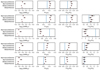 |
Fig. 2 Results of the MCMC retrievals of TiO features in the CARMENES spectrum of GJ 1002 using the narrow and wide spectral ranges and the unfiltered and broadband-filtered versions of the data. Each panel plots the results for a different parameter, which are grouped in columns. The first column contains panels for the fitted
|

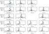 |
Fig. 3 Same as Fig. 2, but for the MCMC retrievals of TiO features in the narrow, broadband-filtered CARMENES spectrum of GJ 1002 with various levels of noise added. The results from the retrieval of the narrow, broadband-filtered spectrum without added noise are shown by the vertical blue lines. |
6.2 GJ 1002 Ti isotope ratios in context
The relative abundances of Ti isotopes in GJ 1002 derived using the four different retrieval setups are all significantly different from the terrestrial values. While 48Ti accounts forabout 74% of all titanium atoms on Earth, we found this value to be only 63–66% in GJ 1002. The minor isotopes were all measured to be about 1–4% more abundant. We compared these values to those measured by Chavez & Lambert (2009) for a sample of 11 K- and M-dwarfs. They found a spread of about 11% in the relative abundance of 48Ti, which is similar to the difference we found between GJ 1002 and Earth. With a literature metallicity of [M ∕H] = +0.20, the lower 48Ti/Ti value we measured for GJ 1002 is consistent with expectations from various Galactic chemical models (e.g., Hughes et al. 2008; Chavez & Lambert 2009), which predict a negative correlation between the relative abundance of 48Ti and metallicity. However, we note that in their stellar sample spanning metallicities − 1 < [Fe∕H] < 0, Chavez & Lambert (2009) found essentially no correlation between metallicity and isotope ratios relative to 48Ti, which are all similar to terrestrial.
As mentioned in Sect. 6.1, though, it is likely the strong 48TiO lines we fit are saturated, so we are cautious to draw firm conclusions from the isotope ratios relative to Ti and 48Ti. On the other hand, the abundances ratios of 47Ti, 49Ti, and 50Ti relative to 46Ti are not expected to be affected by saturation. The fourth column of Fig. 2 indicates 50Ti/46Ti in GJ 1002 to be consistent with the terrestrial value, and the values for 47Ti/46Ti and 49Ti/46Ti to be consistent or marginally higher than Earth. These results are generally consistent with those from Chavez & Lambert (2009), who found approximately terrestrial values across their M-dwarf sample.
6.3 Determining Ti isotope ratios for gas-giant exoplanets
In Sect. 6.1, we show that the loss of continuum information common to exoplanet studies at high resolution should not be prohibitive in deriving Ti isotope ratios for gas-giant exoplanets. The other major difference between TiO analyses of M-dwarfs and future studies of exoplanets is the much fainter signals in the latter case. Figures 3 and 4 demonstrate that even for relatively low S/N levels, it is possible to constrain the relative abundances of Ti isotopes from the narrow and broadband-filtered spectrum and the wide and broadband-filtered spectrum, respectively. For each of the S/N levels shown, the  value of each isotopologue is consistent to within 3σ of the non-degraded results, as are the Ti abundance ratios.
As expected, the fitting errors from the MCMC posteriors increase as the S/N decreases, and they are smaller for the wide, broadband-filtered spectrum compared to those for the narrow, broadband-filtered spectrum at a given S/N. To achieve ≲10% relative error for all Ti isotope ratios, the spectra in the range 7045–7050 Å must have S∕N ≥ 10 for the narrow, broadband-filtered case and S∕N ≥ 5 for the wide, broadband-filtered case.
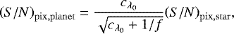
To estimate the integration time required to achieve these S/N for various planetary systems using future high-contrast and high-dispersion instruments such as RISTRETTO (Chazelas et al. 2020) on the Very Large Telescope (VLT) and HIRES (Marconi et al. 2020) on the Extremely Large Telescope (ELT), we used a method similar to that described in Mollière & Snellen (2019). Assuming Poisson noise and negligible sky contribution, the planet emission S/N in a pixel centered at wavelength λ0 is
 (2)
(2)
where  is the stellar S/N in the pixel,
  is the planet-to-star luminosity contrast at wavelength λ0, and f is the stellar-flux-reduction factor used to estimate the effect of suppressed stellar contribution in spatially resolved observations. Following Mollière & Snellen (2019), we adopted f values of 100 and 1000 for spatially resolved observations on the VLT and ELT, respectively, and f =1 for spatially unresolved observations. We approximated
  as the ratio of blackbody luminosities at λ0.
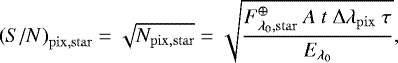
The stellar S/N is related to the integration time t by
 (3)
(3)
where Npix,star is the number of stellar photons collected by the pixel centered at λ0,  is the stellar flux at wavelength λ0 received at Earth, A is the telescope collecting area, Δλpix is the pixel width, τ is the telescope and instrument throughput, and
  is the photon energy at wavelength λ0. Similar to Mollière & Snellen (2019), we took A to be 52 m2 and 976 m2 for the VLT and ELT, respectively, and adopted a throughput of 0.15. We approximated
  using the blackbody luminosity at wavelength λ0. For a given resolving power and number of pixels per resolution element npix, we can write
  . Following Mollière & Snellen (2019), we adopted
  and npix = 3. By replacing forΔλpix, equating Eqs. (2) and (3), and rearranging, the required integration time for a given planet’s S/N is
![Mathematical equation: \begin{equation*}{t}{} = \left[{\left({S/N} \right)_{\mathrm{pix},\mathrm{planet}}}{}\right]^{2} \left(\frac{ {E_{\lambda_0}}{}\ \mathcal{R}\ {n_{\mathrm{pix}}}{} }{ {F_{\lambda_0,\mathrm{star}}^{\oplus}}{}\ {A}{}\ \tau{}\ \lambda_0 } \right) \left(\frac{{c_{\lambda_0}}{} + 1/f}{{c_{\lambda_0}}{}^2}\right). \end{equation*}](/articles/aa/full_html/2021/11/aa41941-21/aa41941-21-eq22.png) (4)
(4)
Based on Eq. (4), deriving Ti isotope ratios in unresolved (f = 1) observations of hot Jupiters is possible, but challenging. This is demonstrated by the case of the WASP-33 system, consisting of the transiting 1.7-RJ ultra-hot-Jupiter WASP-33b (Tday = 3100 K) orbiting its 1.5-R⊙ A5 host star(Teff = 7430 K) in a 1.2-d period (Collier Cameron et al. 2010; Kovács et al. 2013; Nugroho et al. 2021). WASP-33b is, thus far, the only hot Jupiter with evidence for TiO emission based on high-resolution spectral analyses (Nugroho et al. 2017; Serindag et al. 2021; Cont et al. 2021). At a distance of 117 pc (Kovács et al. 2013), to achieve S∕N = 5 at 7045 Å on the ELT requires about seven hours of integration time assuming the planet dayside is fully visible, but nearly 29 h of integration time assuming only half the planet dayside is visible.
Spatially resolved observations decrease the required integration time by reducing stellar contamination, though the planets suitable to such observations necessarily orbit much farther from their host stars than hot Jupiters. However, young wide-orbit planets are known to have Teff similar to ultra-hot Jupiters. For example, the directly imaged 3.4-RJ planet GQ Lupi b has an effective temperature of 2400 K, despite orbiting its 1.7-R⊙ T Tauri K7 host star (Teff = 4300 K) at ~100 AU (Herbig 1977; Lavigne et al. 2009; Donati et al. 2012; Wu et al. 2017). At 150 pc (Crawford 2000), it would take less than one minute of integration time on the ELT to achieve a planet S/N of 5 at 7045 Å. Excitingly, the same S/N would also be attainable on the VLT in about an hour. Thus, there are excellent prospects to determine Ti isotope ratios in young gas-giant exoplanets on wide orbits.
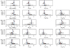 |
Fig. 4 Same as Fig. 3, but for the MCMC retrievals performed on the wide, broadband-filtered CARMENES spectrum of GJ 1002. |
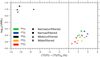 |
Fig. 5 Comparison of absolute and relative abundances derived from each retrieval methodology, demonstrating the small impact the wavelength range and broadband filtering have on the results. For each stable titanium isotope
iTi, the retrieved |

7 Conclusions
We used petitRADTRANS models to fit TiO features in a CARMENES high-resolution spectrum of the M-dwarf GJ 1002, retrieving the relative abundances of Ti isotopes for a narrow and wide wavelength range, and for the unfiltered and broadband-filtered spectrum. The latter mimics typical high-resolution spectra of exoplanets for which continuum information is lost. Differences in the retrieved isotope ratios using the different setups are small. Most affected is the main isotope 48Ti due to possible saturation of the strongest 48TiO lines. By degrading the S/N of the GJ 1002 spectrum and rerunning the retrievals, we determine a planetary S∕N ≥ 5 is necessary to retrieve abundance ratios with relative errors ≲10% when fitting the wide wavelength range 7045–7500 Å. Future spatially resolved high-dispersion observations of wide-orbiting young gas giants can easily achieve such S/N, requiring only an hour and less than a minute of integration time on VLT/RISTRETTO and ELT/HIRES, respectively.
Acknowledgements
D.B.S., I.A.G.S., and P.M. acknowledge support from the European Research Council under the European Union’s Horizon 2020 research and innovation program under grant agreement no. 694513. P.M. acknowledges support from the European Research Council under the European Union’s Horizon 2020 research and innovation program under grant agreement no. 832428.
Appendix A Supplementary materials
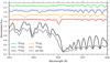 |
Fig. A.1 Flux contribution of each TiO isotopologue (solid lines) to the full TiO spectral model containingall isotopologues (dashed black line) around the strong band head at 7056 Å (7054 Å in air). Abundances were set at the retrieved values presented in Table A.1 for the narrow and unfiltered GJ 1002 spectrum. The flux contribution of a given minor isotopologue iTiO was calculated as the difference between the model of all TiO isotopologues and the model of all isotopologues except iTiO. Since 48TiO comprises 63% of TiO molecules in this setup, its flux contribution (solid black line) was calculated individually, without the presence of the minor isotopologues. Each contribution was normalized based on the full model’s flux to ensure consistent scaling. The minor isotopologue contributions were vertically shifted to aid readability, with the offsets indicated bythe dotted lines. |
Mean parameter values and 1σ errors from MCMC retrievals using different wavelength ranges and broadband filtering
Formal deviation between parameters retrieved using different wavelength ranges and broadband filtering
References
- Altwegg, K., Balsiger, H., Bar-Nun, A., et al. 2015, Science, 347, 1261952 [Google Scholar]
- Asplund, M., Grevesse, N., Sauval, A. J., & Scott, P. 2009, ARA&A, 47, 481 [NASA ADS] [CrossRef] [Google Scholar]
- Ayres, T. R., Lyons, J. R., Ludwig, H. G., Caffau, E., & Wedemeyer-Böhm, S. 2013, ApJ, 765, 46 [NASA ADS] [CrossRef] [Google Scholar]
- Brogi, M., & Line, M. R. 2019, AJ, 157, 114 [Google Scholar]
- Caballero, J. A., Guàrdia, J., del Fresno, M. L., et al. 2016, in Observatory Operations: Strategies, Processes, and Systems VI, 9910, eds. A. B. Peck, R. L. Seaman, & C. R. Benn, International Society for Optics and Photonics (SPIE), 110 [Google Scholar]
- Chavez, J., & Lambert, D. L. 2009, ApJ, 699, 1906 [NASA ADS] [CrossRef] [Google Scholar]
- Chazelas, B., Lovis, C., Blind, N., et al. 2020, in Adaptive Optics Systems VII, 11448, eds. L. Schreiber, D. Schmidt, & E. Vernet, International Society for Optics and Photonics (SPIE), 1393 [Google Scholar]
- Chen, G., Pallé, E., Parviainen, H., Murgas, F., & Yan, F. 2021, ApJ, 913, L16 [NASA ADS] [CrossRef] [Google Scholar]
- Clegg, R. E. S., Lambert, D. L., & Bell, R. A. 1979, ApJ, 234, 188 [NASA ADS] [CrossRef] [Google Scholar]
- Collier Cameron, A., Guenther, E., Smalley, B., et al. 2010, MNRAS, 407, 507 [NASA ADS] [CrossRef] [Google Scholar]
- Cont, D., Yan, F., Reiners, A., et al. 2021, A&A, 651, A33 [NASA ADS] [CrossRef] [EDP Sciences] [Google Scholar]
- Crawford, I. A. 2000, MNRAS, 317, 996 [NASA ADS] [CrossRef] [Google Scholar]
- Donati, J. F., Gregory, S. G., Alencar, S. H. P., et al. 2012, MNRAS, 425, 2948 [Google Scholar]
- Foreman-Mackey, D., Hogg, D. W., Lang, D., & Goodman, J. 2013, PASP, 125, 306 [Google Scholar]
- Fortney, J. J., Lodders, K., Marley, M. S., & Freedman, R. S. 2008, ApJ, 678, 1419 [CrossRef] [Google Scholar]
- Gandhi, S., & Madhusudhan, N. 2019, MNRAS, 485, 5817 [Google Scholar]
- Genda, H., & Ikoma, M. 2008, Icarus, 194, 42 [NASA ADS] [CrossRef] [Google Scholar]
- Gibson, N. P., Merritt, S., Nugroho, S. K., et al. 2020, MNRAS, 493, 2215 [Google Scholar]
- Goodman, J., & Weare, J. 2010, Commun. Appl. Math. Comput. Sci., 5, 65 [Google Scholar]
- Gustafsson, B., Edvardsson, B., Eriksson, K., et al. 2008, A&A, 486, 951 [NASA ADS] [CrossRef] [EDP Sciences] [Google Scholar]
- Hartogh, P., Lis, D. C., Bockelée-Morvan, D., et al. 2011, Nature, 478, 218 [Google Scholar]
- Herbig, G. H. 1977, ApJ, 214, 747 [Google Scholar]
- Hubeny, I., Burrows, A., & Sudarsky, D. 2003, ApJ, 594, 1011 [Google Scholar]
- Hughes, G. L., Gibson, B. K., Carigi, L., et al. 2008, MNRAS, 390, 1710 [NASA ADS] [Google Scholar]
- Jones, A., Noll, S., Kausch, W., Szyszka, C., & Kimeswenger, S. 2013, A&A, 560, A91 [NASA ADS] [CrossRef] [EDP Sciences] [Google Scholar]
- Kovács, G., Kovács, T., Hartman, J. D., et al. 2013, A&A, 553, A44 [Google Scholar]
- Lambert, D. L., & Luck, R. E. 1977, ApJ, 211, 443 [NASA ADS] [CrossRef] [Google Scholar]
- Lambert, D. L., & Mallia, E. A. 1972, MNRAS, 156, 337 [NASA ADS] [CrossRef] [Google Scholar]
- Lavigne, J.-F., Doyon, R., Lafrenière, D., Marois, C., & Barman, T. 2009, ApJ, 704, 1098 [Google Scholar]
- Leya, I., Schönbächler, M., Wiechert, U., Krähenbühl, U., & Halliday, A. N. 2008, Earth Planet. Sci. Lett., 266, 233 [CrossRef] [Google Scholar]
- Lincowski, A. P., Lustig-Yaeger, J., & Meadows, V. S. 2019, AJ, 158, 26 [NASA ADS] [CrossRef] [Google Scholar]
- Linsky, J. L., Draine, B. T., Moos, H. W., et al. 2006, ApJ, 647, 1106 [Google Scholar]
- Marconi, A., Abreu, M., Adibekyan, V., et al. 2020, in Ground-based and Airborne Instrumentation for Astronomy VIII, 11447, eds. C. J. Evans, J. J. Bryant, & K. Motohara, International Society for Optics and Photonics (SPIE), 461 [Google Scholar]
- McKemmish, L. K., Masseron, T., Hoeijmakers, H. J., et al. 2019, MNRAS, 488, 2836 [Google Scholar]
- Meija, J., Coplen, T. B., Berglund, M., et al. 2016, Pure Appl. Chem., 88, 293 [Google Scholar]
- Milam, S. N., Savage, C., Brewster, M. A., Ziurys, L. M., & Wyckoff, S. 2005, ApJ, 634, 1126 [Google Scholar]
- Mollière, P., & Snellen, I. A. G. 2019, A&A, 622, A139 [NASA ADS] [CrossRef] [EDP Sciences] [Google Scholar]
- Mollière, P., van Boekel, R., Dullemond, C., Henning, T., & Mordasini, C. 2015, ApJ, 813, 47 [Google Scholar]
- Mollière, P., Wardenier, J. P., van Boekel, R., et al. 2019, A&A, 627, A67 [Google Scholar]
- Morley, C. V., Skemer, A. J., Miles, B. E., et al. 2019, ApJ, 882, L29 [NASA ADS] [CrossRef] [Google Scholar]
- Noll, S., Kausch, W., Barden, M., et al. 2012, A&A, 543, A92 [NASA ADS] [CrossRef] [EDP Sciences] [Google Scholar]
- Nugroho, S. K., Kawahara, H., Masuda, K., et al. 2017, AJ, 154, 221 [Google Scholar]
- Nugroho, S. K., Kawahara, H., Gibson, N. P., et al. 2021, ApJ, 910, L9 [CrossRef] [Google Scholar]
- Pavlenko, Y. V., Yurchenko, S. N., McKemmish, L. K., & Tennyson, J. 2020, A&A, 642, A77 [NASA ADS] [CrossRef] [EDP Sciences] [Google Scholar]
- Quirrenbach, A., Amado, P. J., Caballero, J. A., et al. 2014, SPIE Conf. Ser., 9147, 91471F [Google Scholar]
- Rajpurohit, A. S., Allard, F., Rajpurohit, S., et al. 2018, A&A, 620, A180 [NASA ADS] [CrossRef] [EDP Sciences] [Google Scholar]
- Romano, D., Matteucci, F., Zhang, Z. Y., Papadopoulos, P. P., & Ivison, R. J. 2017, MNRAS, 470, 401 [NASA ADS] [CrossRef] [Google Scholar]
- Serindag, D. B., Nugroho, S. K., Mollière, P., et al. 2021, A&A, 645, A90 [EDP Sciences] [Google Scholar]
- Spiegel, D. S., Silverio, K., & Burrows, A. 2009, ApJ, 699, 1487 [Google Scholar]
- Trinquier, A., Elliott, T., Ulfbeck, D., et al. 2009, Science, 324, 374 [Google Scholar]
- Valenti, J. A., Piskunov, N., & Johns-Krull, C. M. 1998, ApJ, 498, 851 [Google Scholar]
- Walker, A. R. 1983, South Afr. Astron. Observ. Circ., 7, 106 [Google Scholar]
- Wood, B. E., Linsky, J. L., Hébrard, G., et al. 2004, ApJ, 609, 838 [NASA ADS] [CrossRef] [Google Scholar]
- Wu, Y.-L., Sheehan, P. D., Males, J. R., et al. 2017, ApJ, 836, 223 [CrossRef] [Google Scholar]
- Wyckoff, S., & Wehinger, P. 1972, ApJ, 178, 481 [NASA ADS] [CrossRef] [Google Scholar]
- Zechmeister, M., Reiners, A., Amado, P. J., et al. 2018, A&A, 609, A12 [NASA ADS] [CrossRef] [EDP Sciences] [Google Scholar]
- Zhang, J., Dauphas, N., Davis, A. M., Leya, I., & Fedkin, A. 2012, Nat. Geosci., 5, 251 [NASA ADS] [CrossRef] [Google Scholar]
- Zhang, Y., Snellen, I. A. G., Bohn, A. J., et al. 2021, Nature, 595, 370 [NASA ADS] [CrossRef] [Google Scholar]
Throughout this paper, we exclusively refer to number abundance ratios. For two species, A and B, we abbreviate this by writing A/B.
Molecules comprised of different atomic isotopes, for instance, 47Ti16O versus 48Ti16O.
Based on data from the CARMENES data archive at CAB (INTA-CSIC).
We only differentiate TiO isotopologues based on the stable Ti isotopes. The oxygen isotope fractionation is comparatively negligible.
For brevity, we denote the  for a given isotopologue iTiO as
  .
.
All Tables
Mean parameter values and 1σ errors from MCMC retrievals using different wavelength ranges and broadband filtering
Formal deviation between parameters retrieved using different wavelength ranges and broadband filtering
All Figures
|
Fig. 1 Top left panel: unfiltered CARMENES spectrum of GJ 1002 over the wide wavelength range 7045–7500 Å. The narrow wavelength range 7045–7090 Å is indicated by the blue shading. Top right panel: same as top left panel, but plotting only the narrow wavelength range for clarity. Bottom left panel: broadband-filtered CARMENES spectrum of GJ 1002 over the wide wavelength range. Bottom right panel: same as bottom left panel, but for the narrow wavelength range. |
| In the text | |
|
Fig. 2 Results of the MCMC retrievals of TiO features in the CARMENES spectrum of GJ 1002 using the narrow and wide spectral ranges and the unfiltered and broadband-filtered versions of the data. Each panel plots the results for a different parameter, which are grouped in columns. The first column contains panels for the fitted
|
| In the text | |
|
Fig. 3 Same as Fig. 2, but for the MCMC retrievals of TiO features in the narrow, broadband-filtered CARMENES spectrum of GJ 1002 with various levels of noise added. The results from the retrieval of the narrow, broadband-filtered spectrum without added noise are shown by the vertical blue lines. |
| In the text | |
|
Fig. 4 Same as Fig. 3, but for the MCMC retrievals performed on the wide, broadband-filtered CARMENES spectrum of GJ 1002. |
| In the text | |
|
Fig. 5 Comparison of absolute and relative abundances derived from each retrieval methodology, demonstrating the small impact the wavelength range and broadband filtering have on the results. For each stable titanium isotope
iTi, the retrieved |
| In the text | |
|
Fig. A.1 Flux contribution of each TiO isotopologue (solid lines) to the full TiO spectral model containingall isotopologues (dashed black line) around the strong band head at 7056 Å (7054 Å in air). Abundances were set at the retrieved values presented in Table A.1 for the narrow and unfiltered GJ 1002 spectrum. The flux contribution of a given minor isotopologue iTiO was calculated as the difference between the model of all TiO isotopologues and the model of all isotopologues except iTiO. Since 48TiO comprises 63% of TiO molecules in this setup, its flux contribution (solid black line) was calculated individually, without the presence of the minor isotopologues. Each contribution was normalized based on the full model’s flux to ensure consistent scaling. The minor isotopologue contributions were vertically shifted to aid readability, with the offsets indicated bythe dotted lines. |
| In the text | |
Current usage metrics show cumulative count of Article Views (full-text article views including HTML views, PDF and ePub downloads, according to the available data) and Abstracts Views on Vision4Press platform.
Data correspond to usage on the plateform after 2015. The current usage metrics is available 48-96 hours after online publication and is updated daily on week days.
Initial download of the metrics may take a while.