© P. Hennebelle 2021

1. Introduction

Gravitational collapse is a common and major process that takes place in our Universe. Indeed, all self-gravitating objects such as stars, white dwarfs, neutron stars, or black holes emerge after a phase during which the density of the matter they contain has increased by several orders of magnitude. Other objects such as galaxies, protostellar dense core, as well as proto-stellar cluster clumps and stellar clusters, although less extreme, are also several orders of magnitude denser than the background from which they were assembled by gravity. For many of these objects, turbulence is believed to play a role before or even during the collapse. As a matter of fact, turbulence deeply affects gas dynamics by various effects that depend on the situation. For instance, in the context of star formation, the density fluctuations induced by turbulence within a collapsing core have been proposed to induce fragmentation (e.g., Bate et al. 2003; Goodwin et al. 2004a,b; Lee & Hennebelle 2018a,b; Hennebelle et al. 2019), while in the context of supernova progenitors, density fluctuation generation has been noted as a source of shock distortion that can trigger the explosion (e.g., Foglizzo 2001; Couch & Ott 2013; Müller & Janka 2015). Turbulence within a collapsing prestellar core can also help to transport magnetic flux away (e.g., Santos-Lima et al. 2012; Seifried et al. 2012; Joos et al. 2013), but it may also help to generate magnetic field in primordial clouds through a turbulent dynamo (Schleicher et al. 2010; Federrath et al. 2011; Schober et al. 2012). Turbulence can also strongly influence the angular momentum evolution in a complex manner. Indeed, while generally speaking turbulence can help to transport angular momentum outwards (e.g., Pringle 1981; Balbus & Papaloizou 1999), it can also bring or even generate angular momentum by triggering breakage of axisymmetry (Misugi et al. 2019; Verliat et al. 2020).

Understanding how turbulence behaves during gravitational collapse is therefore of primary importance for a broad range of astrophysical problems. It is also worth mentioning that induced spherical contraction is also most relevant in the context of inertial fusion, for instance. Here, turbulence is again believed to play an important role (Davidovits & Fisch 2016; Viciconte et al. 2018).

To tackle the amplification of turbulence in a compressed medium, Robertson & Goldreich (2012) performed 3D numerical simulations in which the density enhancement is imposed by adding to the fluid equations analytical source terms that describe a homologous contraction (see also Mandal et al. 2020). They also propose an analytical model to describe the behaviour of the turbulent component, which entails a source term induced by the contraction itself and a classical dissipation. By comparing the simulation results and the model, they show that it is able to capture the fluid behaviour well. In the context of the formation of massive stars and the collapse of turbulent cores, Murray & Chang (2015) performed 1D simulations in which the turbulence was modelled using a generalised form of the equation proposed by Robertson & Goldreich (2012), namely

$$\begin{array}{c}\hfill {\partial }_t{V}_T+V_r{\partial }_r{V}_T+\frac{V_T{V}_r}{r}=-\nu \frac{V_T^2}{r}.\end{array}$$(1)

Performing an asymptotic analysis as well as 1D numerical simulations of a spherical collapse with a turbulence described by Eq. (1), they predict typical behaviour of a turbulent collapsing cloud, finding, for instance, density profiles close to but slightly shallower than the classical ρ ∝ r⁻² inferred in isothermal collapse (e.g., Shu 1977). Under the assumption that the turbulent velocity is proportional to the radial ones, Xu & Lazarian (2020) obtained self-similar solutions close to the solutions studied by (Shu 1977).

Recently, Guerrero-Gamboa & Vázquez-Semadeni (2020) performed 3D collapse calculations of an unstable pre-stellar dense core. They found that the turbulence, which develops during the collapse, tends to reach values that are in near virial equilibrium with gravity. They postulate that a local equilibrium between gravitational instability and turbulence is established. A similar conclusion was also reached by Mocz et al. (2017), in which a series of driven turbulence calculations with various magnetisations are presented. Their Fig. 5 unambiguously shows that within collapsing cores, the turbulent pressure is almost proportional to the gravitational energy. In the context of primordial mini halos, similar studies have also been conducted by Higashi et al. (2021), who also found that turbulence is amplified by gravitational contraction. An analytical model based on the growth of gravitational instability is also provided.

All these studies strongly suggest that turbulence is definitely amplified during gravitational collapse. However understanding the mechanism at play precisely remains a challenge because of the great non-linearity of the process. Moreover, so far only a few cases have been explored, while there is a great diversity of initial conditions. The purpose of this study is twofold. First, we inferred a set of 1D equations in spherical geometry that can be seen as a revised version of the equations used, for instance, by Murray & Chang (2015) and Xu & Lazarian (2020). They were inferred by performing a rigorous spherical averaging of the 3D fluid equations. Second, we performed a set of 3D simulations in which we extensively varied the initial conditions but also considered two polytropic equations of state, namely Γ = 1 and Γ = 1.25. Importantly, we performed detailed comparisons between the 1D and 3D simulations, which allowed us to identify the need to add the development of local Jeans instabilities as a source of turbulence when the collapsing cloud is highly unstable. Altogether, the two sets of simulations agree very well, showing that the 1D approach can be used to predict the level of turbulence in collapsing objects.

The plan of the paper is as follows. In the second part of the paper, we discuss how we obtained a set of two equations to describe the evolution of turbulence during gravitational collapse. These equations are close but not identical to the previously proposed equation of Robertson & Goldreich (2012). In the third part, we describe the 1D code that we developed to solve the 1D collapse in spherical geometry taking into account turbulence, and we also describe the 3D simulations that we performed. This includes their setup and how we proceeded to compare the 1D and 3D simulations. In the fourth part, we perform a comparison between the 3D and 1D simulations by comparing the time evolution of the central masses. This leads us to an estimate of the dissipation parameter. In the fifth part, a detailed comparison between 1D and 3D simulations is detailed, and we find that in the proposed equations to describe turbulence, a source term associated with the development of the local Jeans instability is indeed needed to reproduce the 3D simulations. The sixth part is dedicated to a discussion on the nature of the velocity fluctuations. The seventh part concludes the paper.

2. Formalism for turbulence in one-dimensional spherical geometry

We start with a derivation of the 1D equations appropriate to describe a spherical collapsing turbulent cloud.

2.1. Standard equations and spherical mean

While it is clear that in the presence of turbulence the various fields are not spherically symmetric, one can nevertheless consider their spherical mean:

$$\begin{array}{c}\hfill \overline{\rho }={\displaystyle \int \int \mathrm{d}\mathrm{\Omega }\rho ,}{\overline{V}}_r={\displaystyle \int \int \mathrm{d}\mathrm{\Omega }}\frac{\rho }{\overline{\rho }}{V}_r,\end{array}$$(2)

where dΩ = sinθdθdϕ. Similar procedures are employed when inferring sub-grid schemes, for instance (Schmidt et al. 2006).

We introduce the Reynolds decomposition:

$$\begin{array}{c}\hfill V_r={\overline{V}}_r+v_r,\end{array}$$(3)

implying that ${\overline{\mathit{v}}}_r=0$.

To describe turbulence, we also need to consider the orthoradial and azimuthal velocity components V_θ and V_ϕ. Below, we do not need to distinguish between V_θ and V_ϕ and simply consider ${\mathit{v}}_t=\sqrt{V_{\theta }^2+V_{\varphi }^2}$, the transverse velocity component. Our goal is to obtain equations for $\overline{{\mathit{v}}_r^2}$ and $\overline{{\mathit{v}}_t^2}$ separately as they behave differently during the collapse of a spherical cloud.

The continuity equation in spherical geometry is

$$\begin{array}{c}\hfill {\partial }_t\rho +\frac{1}{r^2}{\partial }_r(r^2\rho V_r)+\frac{1}{rsin\theta }{\partial }_{\theta }(sin\theta V_{\theta })+\frac{1}{rsin\theta }{\partial }_{\varphi }{V}_{\varphi }=0.\end{array}$$(4)

With this expression, it is easy to see that when performing the spherical mean as given by Eq. (2), all terms involving angular derivatives cancel out, and thus, for the sake of simplicity, we do not explicitly write the angular-dependent terms below. The other relevant fluid equations are then

$$\begin{array}{c}\hfill {\partial }_t{V}_r+V_r{\partial }_r{V}_r-\frac{v_t^2}{r}=-\frac{1}{\rho }{\partial }_r\left(c_s^2\rho \right)+g_r+\nu {\partial }_r{\sigma }_{\mathit{rr}},\end{array}$$(5)

where c_s is the sound speed, g_r the gravitational acceleration, and σ_rr one of the components of the stress tensor.

$$\begin{array}{c}\hfill {\partial }_t\frac{v_t^2}{2}+V_r{\partial }_r\frac{v_t^2}{2}+\frac{v_t^2{V}_r}{r}=\nu (V_{\theta }{\partial }_r{\sigma }_{r\theta }+V_{\varphi }{\partial }_r{\sigma }_{r\varphi })\end{array}$$(6)

is obtained simply by multiplying the standard orthoradial and azimuthal moment equations by V_θ and V_ϕ, respectively, and adding them.

Finally, the Poisson equation is

$$\begin{array}{c}\hfill \frac{1}{r^2}{\partial }_r\left(r^2{g}_r\right)=-4\pi G\rho .\end{array}$$(7)

2.2. Spherically averaged equations

As explained above, we want to obtain equations on the quantities $\overline{\rho }$, ${\overline{V}}_r$, and $\overline{{\mathit{v}}_T^2}$. Taking the spherical average of Eq. (4), we obtain

$$\begin{array}{c}\hfill {\partial }_t\overline{\rho }+\frac{1}{r^2}{\partial }_r(r^2\overline{\rho }{\overline{V}}_r)=0.\end{array}$$(8)

Next, to obtain a radial mean momentum equation, we first combine Eqs. (4) and (5) to find the conservative form of the following momentum equation:

$$\begin{array}{c}\hfill {\partial }_t(\rho V_r)+\frac{1}{r^2}{\partial }_r(r^2\rho V_r^2)-\frac{\rho v_t^2}{r}=-{\partial }_r\left(c_s^2\rho \right)+\rho g_r+\nu \rho {\partial }_r{\sigma }_{\mathit{rr}},\end{array}$$(9)

then, with the Reynolds decomposition $V_r={\overline{V}}_r+{\mathit{v}}_r$ and after performing the spherical average, we obtained

$$\begin{array}{cc}& {\partial }_t(\overline{\rho }{\overline{V}}_r)+\frac{1}{r^2}{\partial }_r(r^2\overline{\rho }{\overline{V}}_r^2)+\frac{1}{r^2}{\partial }_r(r^2\overline{\rho }\overline{v_r^2})-\frac{\overline{\rho }\overline{v_t^2}}{r}\hfill \\ \hfill & =-{\partial }_r\left(c_s^2\overline{\rho }\right)+\overline{\rho g_r}+\nu \overline{\rho {\partial }_r{\sigma }_{\mathit{rr}}},\hfill \end{array}$$(10)

which can also be written as

$$\begin{array}{cc}& {\partial }_t{\overline{V}}_r+{\overline{V}}_r{\partial }_r{\overline{V}}_r+\frac{2\overline{v_r^2}-\overline{v_t^2}}{r}\hfill \\ \hfill & =-\frac{1}{\overline{\rho }}{\partial }_r((c_s^2+\overline{v_r^2})\overline{\rho })+\frac{\overline{\rho g_r}}{\overline{\rho }}+\frac{\nu \overline{\rho {\partial }_r{\sigma }_{\mathit{rr}}}}{\overline{\rho }}.\hfill \end{array}$$(11)

Next, we sought an equation of $\overline{{\mathit{v}}_r^2}$. For this purpose, we added together the product of Eq. (9) by v_r and the product of Eq. (5) by $V_r={\overline{V}}_r+{\mathit{v}}_r,$ from which we subtracted the product of Eq. (11) by ${\overline{V}}_r$. Finally, we took the spherical mean as defined by Eq. (2), and we obtain the following equation:

$$\begin{array}{cc}& {\partial }_t\left(\frac{\overline{\rho }\overline{v_r^2}}{2}\right)+\frac{1}{r^2}{\partial }_r\left(r^2\frac{\overline{\rho }\overline{v_r^2}}{2}{\overline{V}}_r\right)+\overline{\rho }\overline{v_r^2}{\partial }_r{\overline{V}}_r+\frac{1}{r^2}{\partial }_r\left(r^2\frac{\overline{\rho }\overline{v_r^3}}{2}\right)\hfill \\ \hfill & -\frac{\overline{\rho }\overline{v_t^2{v}_r}}{r}=-\overline{v_r{\partial }_r(c_s^2\rho )}+\overline{v_r\rho g_r}+\nu \overline{v_r\rho {\sigma }_{\mathit{rr}}}.\hfill \end{array}$$(12)

To obtain an equation on $\overline{{\mathit{v}}_t^2}$, we combined Eq. (6) with Eq. (4) and took the spherical mean: this leads to

$$\begin{array}{cc}& {\partial }_t\left(\frac{\overline{\rho }\overline{v_t^2}}{2}\right)+\frac{1}{r^2}{\partial }_r\left(r^2\frac{\overline{\rho }\overline{v_t^2}}{2}{\overline{V}}_r\right)+\frac{\overline{\rho }\overline{v_t^2}{\overline{V}}_r}{r}\hfill \\ \hfill & +\frac{1}{r^2}{\partial }_r\left(r^2\frac{\overline{\rho }\overline{v_t^2{v}_r}}{2}\right)+\frac{\overline{\rho }\overline{v_t^2{v}_r}}{r}=\nu \overline{(v_{\theta }{\partial }_r{\sigma }_{r\theta }+v_{\varphi }{\partial }_r{\sigma }_{r\varphi })}.\hfill \end{array}$$(13)

2.3. Turbulent-kinetic-energy models

Equations (12) and (13) are very similar to the turbulent-kinetic-energy equations obtained in the context of incompressible flow as shown for instance in Eq. (5.132) of Pope (2000). Apart from the Lagrangian derivative, which in the compressible spherically symmetric case is replaced by the second term of the left-hand side, we have one source term that involves $\overline{{\mathit{v}}_r^2}$ and ${\overline{V}}_r$ (third term of the left-hand side) and one term that involves v_r³ or v_t²v_r. It is generally assumed (see Chapt. 10 of Pope 2000) that these terms, together with the pressure ones, lead to an effective turbulent diffusivity; that is, $\propto \mathrm{\nabla }.({\kappa }_T\mathrm{\nabla }\overline{\rho }\overline{{\mathit{v}}^2})$. On the other hand, the last terms on the right hand side represent dissipation that following Robertson & Goldreich (2012) is assumed to be ∝ρv_T²/τ_diss, where τ_diss is the dissipation time. We proceed here with the same assumptions, which lead to

$$\begin{array}{cc}& {\partial }_t\left(\frac{\overline{\rho }\overline{v_r^2}}{2}\right)+\frac{1}{r^2}{\partial }_r\left(r^2\frac{\overline{\rho }\overline{v_r^2}}{2}{\overline{V}}_r\right)+\overline{\rho }\overline{v_r^2}{\partial }_r{\overline{V}}_r\hfill \\ \hfill & +\frac{1}{r^2}{\partial }_r\left(r^3{\eta }_{\mathrm{diff}}{\overline{v_r^2}}^{1/2}{\partial }_r(\overline{\rho }\overline{v_r^2})\right)=-{\eta }_{\mathrm{diss}}\frac{\overline{\rho }\overline{v_r^2}}{{\tau }_{\mathrm{diss}}},\hfill \end{array}$$(14)

$$\begin{array}{cc}& {\partial }_t\left(\frac{\overline{\rho }\overline{v_t^2}}{2}\right)+\frac{1}{r^2}{\partial }_r\left(r^2\frac{\overline{\rho }\overline{v_t^2}}{2}{\overline{V}}_r\right)+\frac{\overline{\rho }\overline{v_t^2}{\overline{V}}_r}{r}\hfill \\ \hfill & +\frac{1}{r^2}{\partial }_r\left(r^3{\eta }_{\mathrm{diff}}{\overline{v_t^2}}^{1/2}{\partial }_r(\overline{\rho }\overline{v_t^2})\right)=-{\eta }_{\mathrm{diss}}\frac{\overline{\rho }\overline{v_t^2}}{{\tau }_{\mathrm{diss}}},\hfill \end{array}$$(15)

where we assumed that ${\kappa }_T={\eta }_{\mathrm{diff}}r{\overline{{\mathit{v}}_T^2}}^{1/2}$ and η_diff is a dimensionless number of the order of a few. We note that to write the dissipation and diffusion terms, it is necessary to estimate the typical dissipation time and diffusion coefficient, and it is generally assumed that the former is simply given by the local crossing time τ_diss = r/v_t, r, while the latter is given by rv_t, r. While these expressions are reasonable, estimating what the relevant spatial scale, that is to say the right r value that should be employed is not a simple task, and this is further discussed in Sect. 3.1.

Equations (14) and (15) are the ones used in this work (however, see the discussion on the generation of turbulence in Sect. 2.4). They are similar to the equation proposed by Robertson & Goldreich (2012) except for the source terms and the turbulent diffusion one. We note, however, that Eqs. (14) and (15) present source terms, namely ρv_r²∂_rV_r and ρv_t²V_r/r, that are not identical. While the second one solely depends on the sign of V_r, the first may be either positive or negative even if V_r remains negative. In particular, during the first phase of the collapse; i.e. before the formation of the central singularity, the amplitude of V_r increases with r (in the cloud inner part), leading to an amplification of v_r while in the second phase, the amplitude of V_r decreases with r. This suggests, as is confirmed later, that the two components behave differently.

Apart from the difference on the turbulent velocity equations, there is another important difference with the equations used, for instance, by Murray & Chang (2015) and Xu & Lazarian (2020), which employed the equation proposed by Robertson & Goldreich (2012) together with a momentum equation that assumed a turbulent pressure ρv_T², where v_T² = v_r² + v_t². From Eq. (11), it is seen that the support provided by turbulence is not identical to theirs if the turbulence is not anisotropic as in this case 2v_r² − v_t² ≠ 0. Even if turbulence is fully isotropic, we note that the turbulent pressure they use is ρv_T², while our analysis suggests that it should be ρv_r² = ρv_T²/3. Generally speaking, it is worth stressing that the support exerted by the transverse component is similar to a centrifugal support apart for the fact that unlike the centrifugal force, it is isotropic. The radial component of the turbulent velocity exerts a support that contains a pressure-like term and a geometric contribution 2v_r²/r.

Finally, we note that at this stage we have two unknowns: η_diss and η_diff. Anticipating our results below, we find that η_diss ≃ 0.25, while we find no evidence that significant turbulent diffusivity should be accounted for.

2.4. Turbulent amplification by local gravitational instability

Equations. (14) and (15) describe the amplification of turbulence, which results from the gravitational compression. It does not take into account the possibility of turbulence being generated by local gravitational instability, as discussed, for instance, in Guerrero-Gamboa & Vázquez-Semadeni (2020). As we see below, this indeed appears to be needed, and to take into account a new source of turbulence in Eqs. (14) and (15), which accounts for the development of local gravitational instabilities on top of the global collapse, we need to estimate the growth rate as a function of time and radius. Generally speaking, this is a complicated problem because the cloud is dynamically evolving. We therefore followed a phenomenological approach. First, we computed the Jeans (Jeans 1902) growth rate as a function of radius:

$$\begin{array}{c}\hfill \omega (r)=\sqrt{4\pi G\rho (r)-c_s^2{(2\pi /2r)}^2}.\end{array}$$(16)

Second, we found the maximum ω_max that occurs at a radius r_max. We assume that as a mode grows, it amplifies the velocity within all points of radius, r <  r_max. Thus,

$$\begin{array}{c}\hfill {\tau }_{\mathrm{jeans}}=1/{\omega }_{max}\mathrm{if}r<r_{max},\\ \hfill {\tau }_{\mathrm{jeans}}=1/\omega (r)\mathrm{if}r>r_{max}.\end{array}$$(17)

This led us to rewrite Eqs. (14) and (15) as

$$\begin{array}{cc}& {\partial }_t\left(\frac{\overline{\rho }\overline{v_r^2}}{2}\right)+\frac{1}{r^2}{\partial }_r\left(r^2\frac{\overline{\rho }\overline{v_r^2}}{2}{\overline{V}}_r\right)+\overline{\rho }\overline{v_r^2}{\partial }_r{\overline{V}}_r\hfill \\ \hfill & =-{\eta }_{\mathrm{diss}}\frac{\overline{\rho }{\overline{v_r^2}}^{3/2}}{r}+\frac{\overline{\rho }\overline{v_r^2}}{2}\frac{1}{{\tau }_{\mathrm{jeans}}}\hfill \end{array}$$(18)

and

$$\begin{array}{cc}& {\partial }_t\left(\frac{\overline{\rho }\overline{v_t^2}}{2}\right)+\frac{1}{r^2}{\partial }_r\left(r^2\frac{\overline{\rho }\overline{v_t^2}}{2}{\overline{V}}_r\right)+\frac{\overline{\rho }\overline{v_t^2}{\overline{V}}_r}{r}\hfill \\ \hfill & =-{\eta }_{\mathrm{diss}}\frac{\overline{\rho }{\overline{v_t^2}}^{3/2}}{r}+\frac{\overline{\rho }\overline{v_t^2}}{2}\frac{1}{{\tau }_{\mathrm{jeans}}}.\hfill \end{array}$$(19)

2.5. A Lagrangian perspective

Equation (19) can be recasted in a different form. By multiplying it by r² and defining J_T = rv_t, we obtain

$$\begin{array}{c}\hfill {\partial }_t\left(\overline{\rho }\overline{J_T^2}\right)+\frac{1}{r^2}{\partial }_r\left(r^2\overline{\rho }\overline{J_T^2}{\overline{V}}_r\right)=-2{\eta }_{\mathrm{diss}}\frac{\overline{\rho }{\overline{J_T^2}}^{3/2}}{r^2}+\frac{\overline{\rho }\overline{J_T^2}}{{\tau }_{\mathrm{jeans}}}.\end{array}$$(20)

If we consider a shell of radius r and thickness dr that we follow in a Lagrangian way, we find that dm = 4πρr²dr is conserved, and therefore

$$\begin{array}{c}\hfill d_t\left(\overline{J_T^2}\right)=-2{\eta }_{\mathrm{diss}}\frac{{\overline{J_T^2}}^{3/2}}{r^2}+\sqrt{4\pi G\rho }\overline{J_T^2},\end{array}$$(21)

where we assumed for the sake of simplicity that ${\tau }_{\mathrm{jeans}}=1/\sqrt{4\pi G\rho }$.

Two possible asymptotic regimes are worth discussing. Assuming stationarity, we thus obtain

$$\begin{array}{c}\hfill \sqrt{\overline{J_T^2}}=\frac{\sqrt{\pi G\rho }{r}^2}{{\eta }_{\mathrm{diss}}},\end{array}$$(22)

while in a situation where gravitational instability does not develop, we obtain

$$\begin{array}{c}\hfill \sqrt{{\overline{J}}_T^2}={(J_{T,0}^{-1}+{\eta }_{\mathrm{diss}}{\displaystyle \int \mathrm{d}t}{r}^{-2})}^{-1};\end{array}$$(23)

that is to say, J_T is continuously decaying.

2.6. Isotropic turbulent equation

If for the sake of simplicity we assume that on average 2v_r is equal to v_t (although we see from Eqs. (12) and (13) that in principle the spherical geometry introduced an isotropy), one can sum up Eqs. (12) and (13) by replacing the third order terms by a turbulent diffusion term and the viscous ones by ηρV_T³/r. We thus obtain

$$\begin{array}{cc}& {\partial }_t\left(\frac{\overline{\rho }\overline{v_T^2}}{2}\right)+\frac{1}{r^2}{\partial }_r\left(r^2\frac{\overline{\rho }\overline{v_T^2}}{2}{\overline{V}}_r\right)+\frac{\overline{\rho }\frac{2}{3}\overline{v_T^2}{\overline{V}}_r}{r}\hfill \\ \hfill & +\overline{\rho }\frac{1}{3}\overline{v_T^2}{\partial }_r{\overline{V}}_r+\frac{1}{r^2}{\partial }_r\left(r^3{\eta }_{\mathrm{diff}}{\overline{v_T^2}}^{1/2}{\partial }_r(\overline{\rho }\overline{v_T^2})\right)\hfill \\ \hfill & =-{\eta }_{\mathrm{diss}}\frac{\overline{\rho }{\overline{v_T^2}}^{3/2}}{r}.\hfill \end{array}$$(24)

3. Codes and setup

Since our goal is to understand the behaviour of turbulence during the gravitational collapse, we performed a set of 1D and 3D simulations, which we closely compare in Sect. 5.

3.1. 1D simulations

We developed a 1D spherical code that solves the set of equations obtained in Sect. 2, namely Eqs. (8), (10), (18), and (19), together with the Poisson equation. The code uses a logarithmic spatial grid and employs vanishing gradient boundary conditions both at the inner and outer boundaries. With a finite volume, the Godunov method is employed with a second-order Muscl-Hancock scheme. The fluxes at the cell interfaces are computed using an Harten-Lax-van Lerr (HLL) solver, which in Cartesian geometry leads to exact conservation of mass, energy, and momentum. We note that Eqs. (10), (18), and (19) entail source terms that cannot be expressed in conservative form.

The code was widely tested using exact homologous collapse solutions that are easy to infer. As the comparisons performed below with the 3D simulations constitute another set of extensive tests, we do not detail them further here.

In Eqs. (14) and (15), the dissipation term is proportional to 1/r. While such a dependence is meaningful once the collapse is fully developed, it is not appropriate before this is the case. In particular, if initially we consider a uniform density, there is no reason why the energy dissipation should be faster in the cloud inner part. To estimate the cloud local dynamical scale, we simply use the density field and write $L_{\mathrm{diss}}=\sqrt{{\rho }_0/\rho }$, where ρ₀ is the initial cloud density.

The spherical mesh extends from 3 10⁻³ × r_c to 5 × r_c, where r_c is the cloud radius. The initial conditions consist of a uniform density medium inside r_c and one hundredth of this value outside the cloud. The radial velocity is initially zero, while the turbulent ones, v_t and v_r are proportional to r^1/3, as expected for a turbulent flow. Their mean values are adjusted in such a way that the mean Mach number inside the cloud is equal to the desired value. We also imposed v_t² = 2v_r² initially.

3.2. 3D simulations

The 3D simulations were performed using the adaptive mesh refinement code Ramses (Teyssier 2002; Fromang et al. 2006). Initially, the computational box, which has a total size equal to 8 × r_c, is described by a grid base of 64³ points (corresponding to level 6 in Ramses). Since we used at least 40 cells per Jeans length, the cloud initially has a resolution that corresponds to level 8, leading to about 64 cells to describe the cloud diameter. As time proceeds, more amr levels are added until level 14 is reached. Finally, once the density reaches a value of 10¹¹ cm⁻³ a Lagrangian sink particle is added (Bleuler & Teyssier 2014).

The initial density distribution is strictly identical to the one of the 1D simulation; i.e. a spherical uniform density cloud 100 times denser than the surrounding medium. One fundamental difference is, however, with the initial turbulence. The velocity field is initialised using a stochastic field that employed random phases and presents a power spectrum with a slope equal to −5/3. This allows us to mimic the expected statistical properties of a turbulent velocity field.

3.3. Runs performed

To understand the behaviour of turbulence within a collapsing cloud, we performed a series of runs and varied three parameters: the mean Mach number, ℳ, the initial ratio of thermal over gravitational energy, α, and the effective adiabatic index. Table 1 summarises the various runs performed. Since all runs are either isothermal or employed an effective polytropic exponent of 1.25, they do not present any characteristic spatial scale and can be freely re-scaled once the value of α is determined. To fix ideas, we choose a mass, M_c, equal to 10  M_⊙ and a radius as specified in Table 1. This is typical of dense prestellar cores (e.g., Ward-Thompson et al. 2007), but we stress that theses results are not restricted to these specific choices and could certainly be applied to objects as different as a collapsing star or a massive star forming clump. For the isothermal runs, the gas temperature was kept fixed to 10 K, while for the run with an effective barotropic equation of state, we simply have T = 10 K (n/n₀)^0.25, where n₀ is the initial cloud density.

As we show below, the thermal-over-gravitational-energy ratio, α, is a key parameter to interpreting the results. Runs A0.5gam1.25M0.1 and A0.5M0.1 initially have α = 0.5 and are therefore near thermal equilibrium, which is generally found for values slightly larger than this. This helps to keep the 3D runs reasonably spherical, which is essential when performing comparisons with the 1D simulations. For the same reason, both runs have a low Mach number equal to 0.1, which makes turbulence of marginal dynamical significance during most of the collapse. The major difference between the two runs is obviously that as the collapse proceeds, the thermal support rapidly drops for run A0.5M0.1. It is well known that

$$\begin{array}{c}\hfill \alpha =\frac{\frac{3}{2}{k}_{\mathrm{B}}T\frac{M_c}{m_p}}{\frac{3G{M}_c^2}{5r_c}}\propto r_c^{4-3\mathrm{\Gamma }}.\end{array}$$(25)

For Γ = 1.25, we have α ∝ r_c^0.25, while for Γ = 1, we have α ∝ r_c. We note that run A0.5gam1.25M0.1 would broadly correspond to a collapsing star on the verge to form a neutron star or a black hole (e.g., Janka et al. 2007) , while run A0.5M0.1 is typical of a low-mass quiescent prestellar dense core (Ward-Thompson et al. 2007).

Runs A0.3M0.1, A0.1M0.1, and A0.02M0.1 also have a Mach numbers of 0.1 initially, but then their initial thermal-over-gravitational energies α are, respectively, 0.3, 0.1, and 0.02. Together with run A0.5M0.1, this allows us to explore an entirely different physical regime.

Finally, runs A0.1M1, A0.1M3, and A0.02M10 have α = 0.1 and α = 0.02 but present Mach numbers that are, respectively, equal to 1, 3, and 10. These initial conditions are more representative of high-mass cores (e.g., Ward-Thompson et al. 2007) or high-mass star forming clumps (e.g., Elia et al. 2017). This is complemented by run A05M1, which presents high thermal and turbulent support and is more representative of lower mass cores. For these three runs, the turbulence is truly dynamically significant. The drawback for the present study is that this induced major departure from the spherical symmetry and this makes the comparison with the 1D simulations less quantitative.

3.4. Choice of time steps and displayed quantities

By performing close comparisons between the two sets of simulations, we expect to accurately test the validity of Eqs. (14) and (15). However, performing such detailed comparisons is not completely straightforward because the collapse time decreases as $1/\sqrt{\rho ,}$ and therefore small differences, due to the intrinsic differences between a 1D configuration and a 3D one, which is not fully spherical, lead to significant shift in time once the collapse is more advanced. For this reason and in order to perform comparisons, we chose to select time steps that have nearly identical central densities before the central sink forms and nearly identical sink masses after it forms. Practically speaking, many time steps of the 1D calculations are stored, and the closest time steps from the 3D ones are chosen. We usually display three time steps before the pivotal stage; i.e. the instant where a singularity forms, which is signed by the appearance of the sink particle, and two time steps after, selecting a sink mass of 0.1–0.2 and ≃1–2  M_⊙, respectively.

For the 1D simulations, the displayed quantities are the directly computed ones; i.e. the density, the radial velocity, the transverse velocity, and the root mean square radial velocity fluctuations. For the 3D simulations, all quantities are computed in concentric shells as the mass weighted mean value. For instance, we have

$$\begin{array}{cc}& v_t^2=\frac{\int \rho {(\mathbf{V}\times \frac{\mathbf{r}}{r})}^2\mathrm{d}\mathrm{\Omega }{r}^2\mathrm{d}r}{\int \rho \mathrm{d}\mathrm{\Omega }{r}^2\mathrm{d}r},\hfill \end{array}$$(26)

$$\begin{array}{cc}& v_r^2=\frac{\int \rho {(\mathbf{V}.\frac{\mathbf{r}}{r}-V_r)}^2\mathrm{d}\mathrm{\Omega }{r}^2\mathrm{d}r}{\int \rho \mathrm{d}\mathrm{\Omega }{r}^2\mathrm{d}r}.\hfill \end{array}$$(27)

The shell centre is chosen to be the most massive sink particle.

4. Estimating turbulent dissipation through a global comparison between 1D and 3D simulations

As mentioned above, we first need to estimate the parameter η_diss, which remains undetermined.

4.1. Previous estimates

Performing non-self-gravitating-driven turbulence simulations, Mac Low (1999) inferred values of the turbulent dissipation. Writing

$$\begin{array}{c}\hfill {\dot{E}}_{\mathrm{turb}}=-\frac{2\pi }{L_d}\eta M{\sigma }^3,\end{array}$$(28)

he inferred η = 0.067, where L_d is the turbulent driving scale.

More recently, Guerrero-Gamboa & Vázquez-Semadeni (2020) discussed turbulent dissipation in a collapsing cloud. By assuming a local energy balance, namely d/dt(E_g/E_turb)=0, and further assuming that the radial and infall speeds are comparable, as confirmed from their simulations, they infer that L_d/R ≃ 8.6η. Thus, the value of η depends on the driving scale. Assuming that L_d = R, they obtained a value of η ≃ 0.12.

Estimating the value of η_diss in a collapsing cloud is not an easy task. In particular, we note that from Eqs. (18) and (19) there are several contributions to the turbulence variations, which is advected, amplified in two different ways in radial and orthoradial directions. These are possibly locally generated if the core is locally gravitationally unstable. As we show later, there are cases where turbulence is amplified but not generated.

We note that from Eqs. (28), (18) and (19), we have 2πη/L_d ≃ η_diss/r. Thus, when assuming that L_d ≃ 2r, i.e., that the driving scale is a local diameter, we obtain η_diss ≃ πη = 0.21.

4.2. Estimating the dissipation parameter

To estimate the value of η_diss, we performed a series of 1D simulations that we compare with the 3D ones. More precisely, for each 3D simulation listed in Table 1, we ran seven 1D simulations for η_diss = 0.1, 0.15, 0.2, 0.25, 0.5, 0.75 and 1. These values were chosen because they fall into the relevant expected range of values from previous studies and because they allow to explore the effects of large changes in turbulent dissipation. A good and important indicator for collapsing clouds is certainly the amount of mass, which has been accreted as a function of time. Indeed, the accreted mass depends on the complete collapse history. Figure 1 portrays the results. The rows and lines respectively correspond to constant initial Mach numbers and constant α values. There is one exception, however: run A01M3 is placed in the bottom and right panels for space reasons.

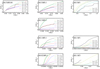Fig. 1. Accreted mass as a function of time for the various 3D simulations performed and labelled in the panel (solid lines) and a series of 1D simulations having the same initial conditions that the 3D ones performed with several values of ηdiss. The dotted lines represent the log of the number of sink particles that form in the 3D simulations.

Obviously, the difficulty in estimating η_diss is that in 3D, the collapse may not remain spherically symmetric, particularly when the turbulent energy is initially high, and this is why several Mach numbers are explored. We start by discussing run A0.5M0.1 (which we remind the reader has α = 0.5 and ℳ = 0.1). The black solid line represents the accreted mass of the 3D simulation, the dotted one is the log of the number of formed sink particles. The dashed and coloured lines represent 1D models with a value of η_diss, as indicated in the legend. As can be seen, the turbulent dissipation parameter, η_diss, appears to play an important role once the collapse has started; i.e. after time t = 0.65 Myr. A remarkable agreement is obtained between the 3D run and the 1D ones, with η_diss = 0.2−0.25 at least up to time t ≃ 0.8 Myr, where M ≃ 2  M_⊙. Interestingly, the behaviour for smaller and larger values of η_diss is quite different. For η_diss <  0.15, the accretion rate is significantly reduced, while for η_diss >  0.25, it is substantially higher. This is clearly a consequence of the turbulence that is, respectively, too strongly dissipated or amplified. While the collapse behaviour strongly depends on η_diss when the value of this parameter is low, the collapse is completely unchanged when η_diss is further increased from 0.5 to 1. This is because the turbulence is so efficiently dissipated that it does not contribute significantly to the collapse.

This conclusion is supported by run A0.5M0.044, which has an initial turbulent energy roughly four times lower than run A0.5M0.1. The collapse with high η_diss is nearly indistinguishable from runs A0.5M0.1 with high η_diss. The dependence on η_diss is also generally similar, although good agreements between 1D and 3D runs are obtained for η_diss ≃ 0.15−0.2, suggesting slightly lower values than for runs A0.5M0.1.

The behaviour of run A0.3M0.1, which has α = 0.3 and ℳ = 0.1, is very similar to run A0.5M0.1. The agreement between the 3D simulation and the 1D one with η_diss = 0.25 appears to be very good.

For run A0.1M0.1, the agreement is also good up to M ≃ 1.5  M_⊙, after which point the 3D simulation accretes much faster. The best value is also clearly η_diss = 0.25. We note that in this run, because of the low thermal energy (α = 0.1), several sink particles have formed, which probably helps to accrete gas more rapidly in the 3D simulation compared to the 1D ones.

Run A0.02M0.1 presents a slightly different behaviour. Generally speaking, the trends are similar, but the effective value of η_diss for which the agreement initially appears to be the best is between 0.1 and 0.15. However, we see that for η_diss = 0.15 the shape of the curve is quite different from the 3D simulation, which appears more compatible with η_diss = 0.2−0.25.

The runs with relatively high Mach numbers, namely A0.5M1, A0.1M1, and A0.1M3, present a significantly different behaviour. They all have the fact that they require much higher values of η_diss >  0.5−1 for the 3D and 1D simulations to match reasonably well in common. Moreover, for small values of η_diss, no central mass forms in the 1D runs. The gas would simply bounce back after some contraction. Clearly, a large dissipation is required to avoid unrealistic turbulent support. The physical interpretation is, however, not straightforward, and as discussed in the next section, it is likely that, at least in part, the high value of η_diss that is needed is a consequence of several sink particles being formed in the 3D runs.

4.3. Turbulent support

It is interesting to compare the timescale for the various runs with same thermal energy but different levels of turbulence, such as A0.5M0.1 with A0.5M1, or A0.1M0.1 and A0.1M1 with A0.1M3. Turbulence typically delays the collapse and slows down accretion, but this delay remains modest. While run A0.1M3 has a turbulent support that is about 30 times larger than that of run A0.1M0.1, the total accreted mass reaches 2  M_⊙, with a delay of only about 10% . As can be seen from Fig. 1, much longer delays are obtained for 1D simulations with smaller η_diss, while for large η_diss the behaviour and the timescale are reasonably well reproduced.

A possible major difference between 1D and 3D simulations is the number of sink particles that the latter are generating. This certainly leads to faster accretion. More generally, this also illustrates the dual role that turbulence is playing by generating density fluctuations that favour local collapses. It is likely that these effects promote the early formation of sink particles and therefore limit the large delay that turbulence would have introduced otherwise.

Similarly, the high value of η_diss seemingly suggested by the comparisons between 1D and 3D A0.1M3 simulations is likely, at least in part, a consequence of the turbulently induced collapse. In principle, a more advanced model could take into account these effects, for instance by computing the probability of finding self-gravitating density fluctuations (e.g., Hennebelle & Chabrier 2008). Moreover, once material has been accreted into a star or sink particles, thermal and turbulent support are retrieved from the gas phase and do not contribute to supporting the gas against gravity.

5. Detailed comparison between 1D and 3D numerical simulations

In this section, we present the detailed results of some of the runs performed. We start with run A0.5M0.1, which is the more thermally supported isothermal run and thus more prone to maintain the spherical symmetry. Then, we present results for A0.1gam1.25M0.1, which has the same initial thermal support as run A0.5M0.1, but since it has Γ = 1.25 the thermal energy during the collapse stays larger. We then study run A0.1M0.1, where thermal support is weak, in more detail. Finally, we end with a discussion on runs with initially high Mach numbers, namely A0.1M1, A0.1M3, and A0.02M10.

5.1. Weak turbulence and high thermal support

5.1.1. Isothermal case

Figure 2 presents the results for run A0.5M0.1 (which has α = 0.5, ℳ = 0.1). Before investigating the agreement between 1D and 3D values, it is worth discussing the results from the 3D calculations (solid lines). The general behaviour displayed by the density, n, and radial velocity, V_r, is typical of collapsing motions. The first three time steps (dark blue and dark red) reveal that in the inner part of the cloud the density is uniform, while the radial velocity remains homologous. Both increase with time. In the outer part of the cloud, both fields connect to the outer values. As already explained, the two last time steps (green and yellow) arise after the pivotal stage (Shu 1977). At these two time steps, the sink particle, which typically represents the central object (say the star or the compact object), has a mass of about 0.2 and 1  M_⊙. Regarding the turbulent components, v_t and v_r, we see that both components are indeed amplified during the collapse, and in the very inner part they reach values comparable to V_r. Also, the two components do not present the same behaviour as anticipated from the different nature of the source terms in Eqs. (14) and (15).

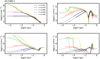Fig. 2. Run A0.5M0.1 (α = 0.5, ℳ = 0.1) at five time steps (3 before and 2 after the sink formation). Full lines: 3D simulations. Dashed lines: 1D simulations. The time steps were adjusted using the value of the central density or the mass of the sink particle. The agreement is generally quite good for the density and radial velocity (except in the cloud’s inner part after sink formation). Before the sink formation, the agreement with the transverse velocity component is also good, though less tight than it is for n and Vr. After the sink formation, we observe major deviations for vt and vr. For the radial velocity fluctuation, vr, the agreement remains comparable to vt except at late time in the cloud inner part and generally outside the cloud (r >  0.1 pc.)

In Fig. 2, the dashed lines represent the 1D calculations that were performed with η_diss = 0.25 (this value is used for all simulations except those from Sect. 5.3). The densities, n, and radial velocities, V_r, of the 1D and 3D calculations agree remarkably well at all time steps. The comparison between the 1D and 3D values of v_t is also remarkably good, though the 3D field presents more fluctuations due to the stochastic nature of turbulence. This is particularly the case before sink formation (black, blue, and red lines). Indeed, after sink formation and at small radii, v_t is higher in the 3D simulations than in the 1D ones. For instance, at time t = 0.709 Myr (yellow line), v_t is up to three times larger in 3D than in 1D simulations. We also see that there is a relatively well defined transition between the outer region, where both values are close, and the inner region, where the 3D values are much larger. This transition propagates from the inside out. Apart from the two last time steps, for which again the values at r <  0.01 pc present major deviations, the agreement is usually better than a few tens of percent, while overall v_t varies by more than one order of magnitude. This demonstrates that Eq. (19) accurately captures the evolution of v_t. We note that for this run, there is actually no difference between Eqs. (15) and (19), because due to the high value of α = 0.5, the source term due to the development of gravitational instability in Eq. (19) is vanishing for all k and all radii r.

The situation for v_r is a little more complex. We see that within the cloud, i.e for r <  0.1 pc, the agreement is still good for the first three time steps (except in a few places), though less accurate than for v_t. Major differences are seen in the outer part of the cloud and almost everywhere at the last time steps. In particular, strong disagreements seem to appear when the radial velocity gradient ∂_rV_r reverses. This suggests that there may be a missing source term that should be added to v_r, perhaps the growth of an instability or the production of sound waves. Indeed, in the context of collapsing stars, it is now well established that acoustic waves can be generated (Abdikamalov & Foglizzo 2020) as a consequence of vorticity conservation.

5.1.2. Γ=1.25

Figure 3 presents the results for run A0.5gam1.25M0.1 (which has α = 0.5, Γ = 1.25, ℳ = 0.1) both for the 3D simulation (solid lines) and the 1D one (dashed one). First of all, a major difference with run A0.5M0.1 needs to be stressed. This regards the duration of the 3D and 1D runs, as the latter is about 40% longer than the former. This seems to be due to the fact that run A0.5gam1.25M0.1 is marginally unstable as it has an exponent close to 4/3 and a high thermal-over-gravitational-energy ratio. Small contrasts, for instance on the gas outside the cloud, have been found to make substantial differences. However, by using the synchronisation procedure based on density, we find, as for run A0.5M0.1, that the overall agreement between 1D and 3D calculations is very good for n and V_r except in the inner part (r <  0.03 pc) well after the sink formation (yellow line). This again is likely because small differences in the inner boundaries (the choice made regarding the sink particle and accretion) are important since the cloud is marginally unstable.

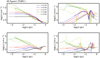Fig. 3. Run A0.5gam1.25M0.1 (α = 0.5, Γ = 1.25, ℳ = 0.1) at five time steps (3 before and 2 after the sink formation). Full lines: 3D simulations. Dashed lines: 1D simulations. The time steps were adjusted using the value of the central density or the mass of the sink particle. As can be seen, the agreement is generally quite good for the density and radial velocity (except in the inner part of the cloud after sink formation). The agreement with the transverse velocity component is also good, though less tight than it is for n and Vr. For the radial velocity fluctuation, vr, the agreement remains comparable to that for vt, except at late time in the inner part of the cloud and generally outside the cloud (r >  0.1 pc.)

The agreement for v_t and v_r is also quite good (except at time t = 0.92 in the cloud inner part for v_t and nearly everywhere for v_r). An important difference with regard to run A0.5M0.1 is that in the 3D simulations, v_t and v_r reach smaller values (up to a factor of 3 below r = 0.01). By contrast, the 1D runs tend to predict similar values for A0.5M0.1 and A0.5gam1.25M0.1.

This clearly indicates that thermal support is making an important difference at the advanced stage of the collapse with regard to turbulent generation. To understand the origin of these differences, Fig. 4 portrays the density cuts as well as the projected velocity field in three snapshots (2 before and 1 after the pivotal stage). As can be seen for the first two snapshots, the clouds remain fairly spherical. However, for the third snapshot the situation is quite different. While for run A0.5gam1.25M0.1 the density field remains spherical, it is not the case in run A0.5M0.1. There, prominent spiral patterns develop. Their origin is very likely due to angular momentum as they are reminiscent of what has been found in many simulations (e.g., Matsumoto & Hanawa 2003; Brucy & Hennebelle 2021). In particular, Verliat et al. (2020) show that the formation of centrifugally supported discs is favoured by symmetry breaking, as in such circumstances the collapse centre is not the centre of mass, and therefore angular momentum is not conserved with respect to the collapse centre. For run A0.5gam1.25M0.1, the thermal support maintains spherical symmetry, preventing prominent axisymmetry breaking.

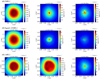Fig. 4. Density and velocity cut at three time steps for runs A0.5M01, A0.5gam1.25M01, and A0.1M01. When thermal energy is high (runs A0.5M01 and A0.5gam1.25M01), the collapse remains symmetric, except after the pivotal stage (top right panel). When thermal energy is low (runs A0.1M01), the collapsing cloud is extremely unstable and non-axisymmetric motions develop even before the pivotal stage.

5.2. Weak turbulence and low thermal support: Turbulent generation

5.2.1. Evidence for another source of turbulence

We started by performing 1D runs with Eqs. (14) and (15), which we remind the reader do not include the generation of turbulence through gravitational instability. Figure 5 presents results for run A0.1M0.1 (which has α = 0.1, Γ = 1, ℳ = 0.1), restricting to the turbulent variables v_r and v_t. Clearly, the 3D values are significantly larger than the 1D ones, even well before reaching the pivotal stage; for instance, this is the case at time t = 0.049 Myr. The disagreement typically increases with time, and unlike what is observed for A0.5M0.1, the amplification does not proceed from the inside out but appears to be global.

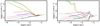Fig. 5. Turbulent components vr and vt for run A0.1M0.1 (α = 0.1, ℳ = 0.1). The 1D simulations were performed with Eqs. (14) and (15); that is to say, without the contribution of the Jeans instability (Eqs. (18) and (19)). The transverse component vt is significantly larger in the 3D calculations than in the 1D ones, implying that another source of turbulence must be accounted for in the 1D simulations.

These results clearly suggest that Eqs. (14) and (15) are missing a source of turbulence. To gain clarity as to what may be happening, Fig. 4 portrays density cuts of run A0.1M0.1. As can be seen, strong non-axisymmetric perturbations develop, therefore generating further turbulence. We note that in run A0.1M0.1 and at 0.045 and 0.049 Myr, the densest density fluctuations, are clearly located in a shell of radius ≃0.01 pc, which is reminiscent of the shell instability known to develop in collapsing clouds with low thermal support (e.g., Ntormousi & Hennebelle 2015).

5.2.2. Evidence for turbulent generation by local gravitational instability

Figure 6 portrays the results of 1D calculations performed with Eqs. (18) and (19) and a value of η_diss = 0.25. Unlike for the 1D simulations displayed in Fig. 5, the contribution of local Jeans instabilities in the development of turbulence is taken into account. The agreement is overall very good. In most locations, and except towards the cloud centre, the 3D and 1D results barely differ by more than a few tens of percent. This clearly shows that turbulence is not only amplified by the contraction, it is also generated by the local development of gravitational instabilities.

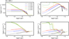Fig. 6. Same as Fig. 2, but for run A0.1M0.1 (α = 0.1, ℳ = 0.1). Unlike in Fig. 5, Eqs. (18) and (19) were used to perform the 1D simulations. The agreement between the 1D (dashed lines) and 3D (solid lines) simulation results is overall very good and much better than when the local Jeans instability is not accounted for, as in Fig. 5.

We note that v_t is possibly a little too high at t = 0.045 and 0.049 Myr and around r ≃ 0.01 pc. This may indicate that the gravitational instability growth rate used in Eqs. (18) and (19) is a little too high there and that a more accurate spatial dependent analysis should be considered (e.g., Nagai et al. 1998; Fiege & Pudritz 2000; Ntormousi & Hennebelle 2015).

5.3. High initial turbulence

In many astrophysical situations of interest, the turbulence is not initially small when the collapse starts, and it is worth investigating to what extent the 1D approach is nevertheless relevant. The obvious difficulty is that when turbulence is strong, it induces major geometrical deviations from spherical geometry, as can be seen from Fig. 7, which displays the column density for runs A.01M1, A0.1M3, and A0.02M10 at three time steps.

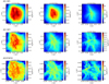Fig. 7. Column density at three time steps of runs A0.1M1, A0.1M3, and A0.02M10. As these runs initially have a high turbulence, the collapsing clouds are extremely non-axisymmetric.

Figure 8 shows the detailed profiles for run A0.1M1 (which has α = 0.1, Γ = 1, ℳ = 1). In this run, the turbulent energy is initially one hundred times larger than in run A0.1M0.1 and initially represents 10% of the gravitational energy. In this section, we use η_diss = 1 as this value is suggested by Fig. 1. In spite of a relatively large initial turbulence, which induces significant departures from spherical geometry (see Fig. 7), the agreement between the 3D and 1D simulations is still remarkably good. In particular, the level of turbulence is close in 3D and 1D runs with a global amplification of the order of a factor of 10 at a few r = 0.001 pc. There is possible discrepancy, on the order of a factor of ≃2 in the inner part and at t = 0.05 Myr, where the 3D turbulence appears to be slightly larger than in the 1D ones. Interestingly, the two components v_r and v_t appear to present profiles much more similar than in runs with lower Mach numbers, where prominent differences between v_r and v_t appear. Notably, we see that the turbulent velocities have amplitudes comparable to the mean radial one, V_r.

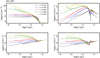Fig. 8. Same as Fig. 2, but for run A0.1M1 (α = 0.1, ℳ = 1). Also, turbulent energy is initially much larger than in run A0.1M0.11.

Figure 9 portrays results for run A0.1M3 (which has α = 0.1, Γ = 1, ℳ = 3). For this run, the turbulent energy is nine times larger than the thermal ones and is therefore comparable to the gravitational energy. As expected, we see from Fig. 7 that the collapse proceeds in a highly non-symmetric way. In spite of this major departure from spherical symmetry, the agreement between 1D and 3D fields is still reasonably good in spite of the high level of fluctuations present in the 3D run.

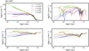Fig. 9. Same as Fig. 2, but for run A0.1M3 (α = 0.1, ℳ = 3). Since the turbulence is strong initially, the collapse proceeds in a non-symmetric way, and therefore the agreement cannot be quantitative. Qualitatively, the 1D and 3D solutions remain similar.

Figure 10 portrays results for run A0.02M10 (which has α = 0.02, Γ = 1, ℳ = 10). This run has a thermal energy that is initially only one percent of the turbulent one, while the latter is comparable to the gravitational energy. As for Fig. 9, we see that the agreement between 1D and 3D runs remains entirely reasonable.

Fig. 10. Same as Fig. 2, but for run A0.02M10 (α = 0.02, ℳ = 10).

6. Discussion

We present quantitative evidence that the velocity fluctuations are greatly amplified within a collapsing cloud. However, the exact nature of these velocity fluctuations requires a better description. In particular, while given our general understanding of fluid behaviour it sounds likely that turbulence is developing, the exact way that the cascade may proceed and what the driving scale is constitute interesting avenues for future investigations. While these questions are beyond the scope of the present paper and clearly require detailed investigations, several aspects can already be discussed.

First of all, the modelling of the turbulent dissipation used in this work appears to play a decisive role. In the absence of dissipation for instance (η_diss = 0), we observe that the collapse is quickly halted and the 1D models do not resemble the 3D ones. On the other hand, when a sufficiently high value of η_diss is used, the agreement between 1D and 3D models become really good. Since the 3D simulations do not have explicit viscosity, numerical dissipation that occurs at the mesh scale is the only dissipation channel. This is a strong indication that a turbulent cascade is taking place. Moreover, at least for low Mach values, the value of η_diss for which the best agreement between 1D and 3D simulations is obtained, appears to be close to the value inferred from 3D compressible turbulence simulations.

Secondly, we can refer to the study of Higashi et al. (2021), where power spectra of kinetic energy have been measured. For instance, from their Figure 9 they inferred that both the compressible and solenoidal modes are amplified and present power spectra close to k^−2, which has been inferred in compressible simulations (e.g., Kritsuk et al. 2007). Things are clearly more complex, however. For instance, starting from velocity fluctuations that present an energy power spectra proportional to k⁻³ instead of k⁻², Higashi et al. (2021) found that it remains proportional to k⁻³ at a low density, but it becomes flatter at a higher density, where it is closer to k⁻².

As a matter of fact, there are likely several regimes of turbulence taking place in collapsing clouds. When turbulence is initially weak, there is a transition between the outer and inner parts of the cloud. This is because, in the latter one, turbulence likely is amplified up to values comparable to gravitational energy. When turbulence is weak, as we saw above, it is likely highly anisotropic, the radial and transverse components having different source terms. Even when turbulence is initially strong and likely more homogeneous and less spatially dependent (see for instance Figs. 9 and 10), turbulence likely remains anisotropic because the mean radial velocity never vanishes and is of comparable amplitude to the other velocity components.

7. Conclusion

We inferred a new set of 1D equations that describe the evolution of the spherically averaged variables during the collapse of a turbulent cloud. These equations, while similar, present significant differences compared to the ones used in the literature. We developed a 1D code that solves these equations, and we performed a series of 1D and 3D simulations. To carry out the latter, the Ramses code was used. The simulation sample covers a wide range of Mach numbers and thermal support expressed by the parameter α and the ratio between thermal and gravitational energy. For each set of initial conditions, we performed several 1D runs with different values of η_diss, which controls the turbulent dissipation. By comparing the central mass as a function of time in 1D and 3D simulations, we can determine that the value of η_diss needed to obtain a good agreement between the 1D and 3D runs is about 0.2–0.25 for low initial Mach numbers. This value is in good agreement with previous estimates inferred for turbulent non-self-gravitating gas. For larger initial Mach numbers, we find that values of η_diss up to five times larger are required to obtain a good match between 1D and 3D simulations. For several sets of initial conditions, we then performed detailed comparisons between the 1D and 3D simulations using the previously inferred values of η_diss. Generally speaking, we obtain remarkable agreement between the 1D and 3D runs. From these detailed comparisons, we show that when the thermal support is significant, initial turbulence is amplified by the collapsing motions. However, when thermal support is low, it is shown that amplification is not sufficient to reproduce the 3D simulations. When turbulent generation through the development of local gravitational instabilities is accounted for, very good agreement between the 1D and 3D runs is obtained. Finally, we show that even when turbulence is initially strong, the spherically averaged equations still predict behaviours that remain quantitatively similar to the 3D simulations. The spherically averaged 1D equations can be used in various contexts to predict the amplification and generation of turbulence within collapse.

Acknowledgments

I thank the referee for their useful report as well as Thierry Foglizzo for enlightening discussions. This work was granted access to HPC resources of CINES and CCRT under the allocation x2014047023 made by GENCI (Grand Equipement National de Calcul Intensif). This research has received funding from the European Research Council synergy grant ECOGAL (Grant : 855130).

References

All Tables

All Figures

	Fig. 1. Accreted mass as a function of time for the various 3D simulations performed and labelled in the panel (solid lines) and a series of 1D simulations having the same initial conditions that the 3D ones performed with several values of ηdiss. The dotted lines represent the log of the number of sink particles that form in the 3D simulations.
In the text

Fig. 2. Run A0.5M0.1 (α = 0.5, ℳ = 0.1) at five time steps (3 before and 2 after the sink formation). Full lines: 3D simulations. Dashed lines: 1D simulations. The time steps were adjusted using the value of the central density or the mass of the sink particle. The agreement is generally quite good for the density and radial velocity (except in the cloud’s inner part after sink formation). Before the sink formation, the agreement with the transverse velocity component is also good, though less tight than it is for n and Vr. After the sink formation, we observe major deviations for vt and vr. For the radial velocity fluctuation, vr, the agreement remains comparable to vt except at late time in the cloud inner part and generally outside the cloud (r >  0.1 pc.)

In the text

Fig. 3. Run A0.5gam1.25M0.1 (α = 0.5, Γ = 1.25, ℳ = 0.1) at five time steps (3 before and 2 after the sink formation). Full lines: 3D simulations. Dashed lines: 1D simulations. The time steps were adjusted using the value of the central density or the mass of the sink particle. As can be seen, the agreement is generally quite good for the density and radial velocity (except in the inner part of the cloud after sink formation). The agreement with the transverse velocity component is also good, though less tight than it is for n and Vr. For the radial velocity fluctuation, vr, the agreement remains comparable to that for vt, except at late time in the inner part of the cloud and generally outside the cloud (r >  0.1 pc.)

In the text

	Fig. 4. Density and velocity cut at three time steps for runs A0.5M01, A0.5gam1.25M01, and A0.1M01. When thermal energy is high (runs A0.5M01 and A0.5gam1.25M01), the collapse remains symmetric, except after the pivotal stage (top right panel). When thermal energy is low (runs A0.1M01), the collapsing cloud is extremely unstable and non-axisymmetric motions develop even before the pivotal stage.
In the text

Fig. 5. Turbulent components vr and vt for run A0.1M0.1 (α = 0.1, ℳ = 0.1). The 1D simulations were performed with Eqs. (14) and (15); that is to say, without the contribution of the Jeans instability (Eqs. (18) and (19)). The transverse component vt is significantly larger in the 3D calculations than in the 1D ones, implying that another source of turbulence must be accounted for in the 1D simulations.

In the text

	Fig. 6. Same as Fig. 2, but for run A0.1M0.1 (α = 0.1, ℳ = 0.1). Unlike in Fig. 5, Eqs. (18) and (19) were used to perform the 1D simulations. The agreement between the 1D (dashed lines) and 3D (solid lines) simulation results is overall very good and much better than when the local Jeans instability is not accounted for, as in Fig. 5.
In the text

	Fig. 7. Column density at three time steps of runs A0.1M1, A0.1M3, and A0.02M10. As these runs initially have a high turbulence, the collapsing clouds are extremely non-axisymmetric.
In the text

	Fig. 8. Same as Fig. 2, but for run A0.1M1 (α = 0.1, ℳ = 1). Also, turbulent energy is initially much larger than in run A0.1M0.11.
In the text

	Fig. 9. Same as Fig. 2, but for run A0.1M3 (α = 0.1, ℳ = 3). Since the turbulence is strong initially, the collapse proceeds in a non-symmetric way, and therefore the agreement cannot be quantitative. Qualitatively, the 1D and 3D solutions remain similar.
In the text

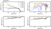	Fig. 10. Same as Fig. 2, but for run A0.02M10 (α = 0.02, ℳ = 10).
In the text

References

- Abdikamalov, E., & Foglizzo, T. 2020, MNRAS, 493, 3496 [NASA ADS] [CrossRef] [Google Scholar]
- Balbus, S. A., & Papaloizou, J. C. B. 1999, ApJ, 521, 650 [Google Scholar]
- Bate, M. R., Bonnell, I. A., & Bromm, V. 2003, MNRAS, 339, 577 [NASA ADS] [CrossRef] [Google Scholar]
- Bleuler, A., & Teyssier, R. 2014, MNRAS, 445, 4015 [Google Scholar]
- Brucy, N., & Hennebelle, P. 2021, MNRAS, 503, 4192 [NASA ADS] [CrossRef] [Google Scholar]
- Couch, S. M., & Ott, C. D. 2013, ApJ, 778, L7 [NASA ADS] [CrossRef] [Google Scholar]
- Davidovits, S., & Fisch, N. J. 2016, Phys. Rev. Lett., 116, 105004 [CrossRef] [Google Scholar]
- Elia, D., Molinari, S., Schisano, E., et al. 2017, MNRAS, 471, 100 [NASA ADS] [CrossRef] [Google Scholar]
- Federrath, C., Chabrier, G., Schober, J., et al. 2011, Phys. Rev. Lett., 107, 114504 [NASA ADS] [CrossRef] [Google Scholar]
- Fiege, J. D., & Pudritz, R. E. 2000, MNRAS, 311, 105 [NASA ADS] [CrossRef] [Google Scholar]
- Foglizzo, T. 2001, A&A, 368, 311 [NASA ADS] [CrossRef] [EDP Sciences] [Google Scholar]
- Fromang, S., Hennebelle, P., & Teyssier, R. 2006, A&A, 457, 371 [NASA ADS] [CrossRef] [EDP Sciences] [Google Scholar]
- Goodwin, S. P., Whitworth, A. P., & Ward-Thompson, D. 2004a, A&A, 414, 633 [NASA ADS] [CrossRef] [EDP Sciences] [Google Scholar]
- Goodwin, S. P., Whitworth, A. P., & Ward-Thompson, D. 2004b, A&A, 423, 169 [NASA ADS] [CrossRef] [EDP Sciences] [Google Scholar]
- Guerrero-Gamboa, R., & Vázquez-Semadeni, E. 2020, ApJ, 903, 136 [NASA ADS] [CrossRef] [Google Scholar]
- Hennebelle, P., & Chabrier, G. 2008, ApJ, 684, 395 [Google Scholar]
- Hennebelle, P., Lee, Y.-N., & Chabrier, G. 2019, ApJ, 883, 140 [Google Scholar]
- Higashi, S., Susa, H., & Chiaki, G. 2021, ApJ, 915, 107 [NASA ADS] [CrossRef] [Google Scholar]
- Janka, H. T., Langanke, K., Marek, A., Martínez-Pinedo, G., & Müller, B. 2007, Phys. Rep., 442, 38 [NASA ADS] [CrossRef] [Google Scholar]
- Jeans, J. H. 1902, Phil. Trans. R. Soc. London Series A, 199, 1 [CrossRef] [Google Scholar]
- Joos, M., Hennebelle, P., Ciardi, A., & Fromang, S. 2013, A&A, 554, A17 [NASA ADS] [CrossRef] [EDP Sciences] [Google Scholar]
- Kritsuk, A. G., Norman, M. L., Padoan, P., & Wagner, R. 2007, ApJ, 665, 416 [NASA ADS] [CrossRef] [Google Scholar]
- Lee, Y.-N., & Hennebelle, P. 2018a, A&A, 611, A88 [NASA ADS] [CrossRef] [EDP Sciences] [Google Scholar]
- Lee, Y.-N., & Hennebelle, P. 2018b, A&A, 611, A89 [NASA ADS] [CrossRef] [EDP Sciences] [Google Scholar]
- Mac Low, M.-M. 1999, ApJ, 524, 169 [Google Scholar]
- Mandal, A., Federrath, C., & Körtgen, B. 2020, MNRAS, 493, 3098 [Google Scholar]
- Matsumoto, T., & Hanawa, T. 2003, ApJ, 595, 913 [Google Scholar]
- Misugi, Y., Inutsuka, S.-I., & Arzoumanian, D. 2019, ApJ, 881, 11 [NASA ADS] [CrossRef] [Google Scholar]
- Mocz, P., Burkhart, B., Hernquist, L., McKee, C. F., & Springel, V. 2017, ApJ, 838, 40 [Google Scholar]
- Müller, B., & Janka, H. T. 2015, MNRAS, 448, 2141 [CrossRef] [Google Scholar]
- Murray, N., & Chang, P. 2015, ApJ, 804, 44 [NASA ADS] [CrossRef] [Google Scholar]
- Nagai, T., Inutsuka, S.-I., & Miyama, S. M. 1998, ApJ, 506, 306 [NASA ADS] [CrossRef] [Google Scholar]
- Ntormousi, E., & Hennebelle, P. 2015, A&A, 574, A130 [NASA ADS] [CrossRef] [EDP Sciences] [Google Scholar]
- Pope, S. B. 2000, Turbulent Flows () [Google Scholar]
- Pringle, J. E. 1981, ARA&A, 19, 137 [NASA ADS] [CrossRef] [Google Scholar]
- Robertson, B., & Goldreich, P. 2012, ApJ, 750, L31 [Google Scholar]
- Santos-Lima, R., de Gouveia Dal Pino, E. M., & Lazarian, A. 2012, ApJ, 747, 21 [NASA ADS] [CrossRef] [Google Scholar]
- Schleicher, D. R. G., Banerjee, R., Sur, S., et al. 2010, A&A, 522, A115 [NASA ADS] [CrossRef] [EDP Sciences] [Google Scholar]
- Schmidt, W., Niemeyer, J. C., & Hillebrandt, W. 2006, A&A, 450, 265 [NASA ADS] [CrossRef] [EDP Sciences] [Google Scholar]
- Schober, J., Schleicher, D., Federrath, C., et al. 2012, ApJ, 754, 99 [NASA ADS] [CrossRef] [Google Scholar]
- Seifried, D., Banerjee, R., Pudritz, R. E., & Klessen, R. S. 2012, MNRAS, 423, L40 [NASA ADS] [CrossRef] [Google Scholar]
- Shu, F. H. 1977, ApJ, 214, 488 [Google Scholar]
- Teyssier, R. 2002, A&A, 385, 337 [NASA ADS] [CrossRef] [EDP Sciences] [Google Scholar]
- Verliat, A., Hennebelle, P., Maury, A. J., & Gaudel, M. 2020, A&A, 635, A130 [EDP Sciences] [Google Scholar]
- Viciconte, G., Gréa, B.-J., & Godeferd, F. S. 2018, Phys. Rev. E, 97, 023201 [NASA ADS] [CrossRef] [Google Scholar]
- Ward-Thompson, D., André, P., Crutcher, R., et al. 2007, Protostars and Planets V, 33 [Google Scholar]
- Xu, S., & Lazarian, A. 2020, ApJ, 890, 157 [Google Scholar]