| Issue |
A&A
Volume 655, November 2021
|
|
|---|---|---|
| Article Number | A70 | |
| Number of page(s) | 9 | |
| Section | Cosmology (including clusters of galaxies) | |
| DOI | https://doi.org/10.1051/0004-6361/202141251 | |
| Published online | 19 November 2021 | |
Hint of a truncated primordial spectrum from the CMB large-scale anomalies
1
Department of Physics, The Applied Math Program, and Department of Astronomy, The University of Arizona, Tucson, AZ 85721, USA
e-mail: This email address is being protected from spambots. You need JavaScript enabled to view it.
2
Guizhou Provincial Key Laboratory of Radio Astronomy and Data Processing, and School of Physics and Electronic Science, Guizhou Normal University, Guiyang 550001, PR China
3
Purple Mountain Observatory, Chinese Academy of Sciences, Nanjing 210023, PR China
4
Guangxi Key Laboratory for Relativistic Astrophysics, Guangxi University, Nanning 530004, PR China
5
University of Chinese Academy of Sciences, Beijing 100049, PR China
Received:
4
May
2021
Accepted:
12
September
2021
Abstract
Context. Several satellite missions have uncovered a series of potential anomalies in the fluctuation spectrum of the cosmic microwave background temperature, including: (1) an unexpectedly low level of correlation at large angles, manifested via the angular correlation function, C(θ); and (2) missing power in the low multipole moments of the angular power spectrum, Cℓ.
Aims. Their origin is still debated, however, due to a persistent lack of clarity concerning the seeding of quantum fluctuations in the early Universe. A likely explanation for the first of these appears to be a cutoff, kmin = (3.14 ± 0.36)×10−4 Mpc−1, in the primordial power spectrum, 𝒫(k). Our goal in this paper is twofold: (1) we examine whether the same kmin can also self-consistently explain the missing power at large angles, and (2) we confirm that the introduction of this cutoff in 𝒫(k) does not adversely affect the remarkable consistency between the prediction of Planck-ΛCDM and the Planck measurements at ℓ > 30.
Methods. We have used the publicly available code CAMB to calculate the angular power spectrum, based on a line-of-sight approach. The code was modified slightly to include the additional parameter (i.e., kmin) characterizing the primordial power spectrum. In addition to this cutoff, the code optimized all of the usual standard-model parameters.
Results. In fitting the angular power spectrum, we found an optimized cutoff, kmin = (2.04−0.79+1.4) × 10−4 Mpc−1, when using the whole range of ℓ’s, and kmin = (3.3−1.3+1.7) × 10−4 Mpc−1, when fitting only the range ℓ ≤ 30, where the Sachs-Wolfe effect is dominant.
Conclusions. These are fully consistent with the value inferred from C(θ), suggesting that both of these large-angle anomalies may be due to the same truncation in 𝒫(k).
Key words: cosmic background radiation / cosmological parameters / cosmology: theory / cosmology: observations / large-scale structure of Universe
John Woodruff Simpson Fellow.
© ESO 2021
1. Introduction
All three major satellite missions designed to study the cosmic microwave background (CMB) – COBE (Hinshaw et al. 1996), WMAP (Bennett et al. 2003), and Planck (Planck Collaboration VII 2020) – have uncovered several unexpected features in its temperature fluctuations. These include missing correlations at large angles and an unexpectedly low power in multipoles 2 ≲ ℓ ≲ 30, especially ℓ = 2 and 3. In spite of these apparent deficiencies, however, the agreement between the angular power spectrum predicted by ΛCDM and the observations is quite remarkable for ℓ > 30, forming the basis for the optimization of many cosmological parameters.
The large-scale anomalies stand in sharp contrast to the general level of success interpreting the CMB anisotropies, sustaining a simmering debate concerning their origin, or possible misidentification due to unknown systematic effects (see Bennett et al. 2011; Copi et al. 2010 for reviews). If these two unexpected features are real, it is not even clear if they are due to the same physical process, in spite of the fact that they both characterize variations in temperature over very large angular scales.
A thorough analysis of these anomalies was carried out with the final release of the Planck data by the Planck Collaboration VII (2020). They studied the statistical isotropy and Gaussianity of the CMB using both the Planck 2018 temperature and polarization data. Previous work had focused solely on the temperature fluctuations, due to only a limited ability to also probe the CMB polarization. The large-angular-scale polarization measurements permit a largely independent examination of the peculiar features seen in the temperature which can, in principle, reduce or eliminate any subjectivity or ambiguity in interpreting their statistical significance.
The possibility that the lack of large-angle correlations in the temperature may be largely due to a statistical “fluke”, as unlikely as that may appear to be, was raised by the fact that the Planck Collaboration VII study found only weaker evidence of an analogous lack of large-scale angular correlations in the polarization data.
Nevertheless, in spite of the fact that no unambiguous detections of cosmological non-Gaussianity, or of anomalies analogous to those seen in temperature, could be claimed, efforts at reducing the systematic effects that contaminated the earlier polarization maps on large angular scales could not completely exclude the presence of residual systematics that limit some tests of non-Gaussianity and isotropy.
A comparison of both the temperature and polarization analyses thus tends to mitigate our ability to conclude one way or the other whether the large-angle anomalies are real. From a theoretical standpoint, the polarization fluctuations also originated in the primordial gravitational potential, but are largely sourced by different modes than the temperature anisotropies. Thus, a measurement of large-scale anomalies in both the temperature and polarization has the potential of providing a greater statistical significance. It is important to see whether any anomalies seen in the polarization maps are related to known features in the temperature. On the other hand, if no such anomalies are seen in the polarization it might be the case that the temperature anomalies, if not pure flukes, could be due to secondary influences, such as the integrated Sachs-Wolfe effect (Planck Collaboration XXI 2016), or more exotic scenarios in which they may be due to physical processes that do not correlate with the polarization.
The situation with regard to the large-angle anomalies is thus far from clear, and it is essential to continue broadening the study of possible causes of such features in either the temperature, polarization or both. In earlier work (Melia & López-Corredoira 2018), we showed that a likely theoretical explanation for the missing large-angle correlations in temperature is the presence of a cutoff, kmin, in the primordial power spectrum, 𝒫(k). Indeed, our analysis of the Planck data revealed that a zero cutoff is ruled out by these measurements at a confidence level ≳8σ. Instead, we found that the observed angular correlation function, C(θ), could be reproduced satisfactorily at all angles with a cutoff kmin = (4.34 ± 0.50)/rdec, where rdec is the comoving distance between us and the last scattering surface at decoupling (zdec = 1080). A truncation such as this is not necessarily consistent with the aims of slow-roll inflation to simultaneously fix the horizon problem and seed a quantum fluctuation spectrum consistent with large-scale structure (Liu & Melia 2020; Melia 2020), because kmin represents the time at which inflation could have started, severely constraining the number of e-folds available for the Universe to expand at an accelerated rate. It is therefore imperative to pursue this line of inquiry further and see if additional evidence may be found in favor of a non-zero kmin.
The goal of this paper is to complete that analysis in two significant ways: (1) to examine whether the same cutoff may be responsible for both large-angle anomalies, and (2) to confirm that the introduction of kmin in 𝒫(k) does not adversely impact the remarkable agreement between theory and observations at ℓ > 30. In Sect. 2 we introduce the basic theoretical background underlying this work, and then proceed to study the effects of a truncated 𝒫(k) on the angular power spectrum in Sect. 3. We discuss the results in Sect. 4, and present our conclusion in Sect. 5.
2. Theoretical background
The inflationary paradigm posits that an early accelerated expansion persisted long enough to create a homogeneous and isotropic Universe within our current Hubble volume. As such, the CMB temperature, T, measured in some direction  , is expected to be a Gaussian random field on the sky, expandable as a series of spherical harmonics,
  , with independent Gaussian random coefficients aℓm of zero mean:
 (1)
(1)
for all ℓ > 0 and m = −ℓ, − ℓ + 1, ..., +ℓ. If the Universe is indeed statistically isotropic, this spherical harmonic decomposition, and the two-point angular power spectrum derived from it, contain all of the physical information needed to interpret the CMB anisotropies.
The less used (but equally important) angular correlation function C(θ) relates the temperature measured in two independent directions,  and
and  , and depends solely on the dot product
  . One may thus expand it in terms of Legendre polynomials:
 (2)
(2)
in which the variance Cℓ is known as the angular power of multipole ℓ. Statistical independence implies that the expectation of a product of aℓm’s with different ℓ’s and m’s vanishes, while isotropy requires the constant of proportionality for this product to be solely a function of ℓ, not m:
 (3)
(3)
As one can see from Fig. 1 (discussed below), the standard model has been strikingly successful in accounting for the angular power spectrum (i.e., Cℓ versus ℓ), at least on small angular scales (≲1°), corresponding to ℓ ≳ 100. The rather precise determination of the various cosmological parameters (Planck Collaboration VI 2020) is based on this excellent agreement between theory and observation.
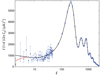 |
Fig. 1. Angular power spectrum (blue dots) estimated with the NLIC method, with 1σ Fisher errors. These error bars include cosmic variance, approximated as Gaussian (see Fig. 1 in Planck Collaboration VI 2020). The ΛCDM best fit model ( |


In principle, the angular correlation function C(θ) contains the same information as the angular power spectrum (see Eq. (2)), but there are good reasons for analyzing the CMB anisotropies separately using these two approaches. First, whereas the angular power spectrum highlights the relative contributions of different spherical harmonics, the angular correlation function describes the variations of T in real space. Some features may emerge more prominently in one description than the other. Second, C(θ) highlights properties of the anisotropies at relatively large angles (i.e., small ℓ’s), while the power spectrum provides ample detail in the opposite regime, namely ℓ ≫ 10. One can easily see the reason for this with a quick inspection of Fig. 1. When using the full angular power spectrum, the model fit is dominated by over 1000 values of ℓ at ℓ > 30, and while the optimized fit is striking in this regime, as we discuss elsewhere in this paper, the error bars and variance at ℓ < 30 are much larger and the fit is significantly less compelling. On the other hand, the angular correlation function displays the temperature anisotropies with equal weighting over all angles 0 ≤ θ ≤ 180°. When fitting a model to these data, the dominant influence is therefore at θ > 10°, the opposite of what happens with the power spectrum. Third, C(θ) is a direct pixel-based measure, not requiring any reconstruction of the observed sky. Some of the systematics may therefore have less impact in one approach relative to the other.
In spite of these differences, one may nonetheless reasonably expect that, of the various large-angle anomalies seen in the CMB (Planck Collaboration VII 2020), the one associated with C(θ) could have the same physical origin as a second emerging from the angular power spectrum. Many authors (see, e.g., Copi et al. 2010) have pointed out that the most striking feature of the angular correlation function (as seen, say, in Fig. 2 of Melia & López-Corredoira 2018) is not just that it disagrees with ΛCDM at a very high level of confidence (≳3σ; Copi et al. 2015), but that it is nearly zero at large angles (≳60°)–in significant tension with inflation, which should have produced correlations throughout the visible Universe.
Most of the statistical weight in the Planck analysis of the angular power spectrum is provided by the high-ℓ multipoles, and one may see in Fig. 1 that the best-fitting portion of the curve traces the data at ℓ ≳ 60 much better than those at low-ℓ’s. Indeed, a general lack of angular power appears within the range 2 ≲ ℓ ≲ 30–especially with the quadrupole ℓ = 2–at a confidence level exceeding 99% (Bennett et al. 2011; Planck Collaboration VI 2020). Quite remarkably, none of the attempted fixes invoking physically motivated inputs, such as neutrino properties, the number of relativistic degrees of freedom, or a running of the spectral index in the fluctuation distribution, have provided any significant improvement to the fit (see, e.g., Planck Collaboration XXIV 2014; Planck Collaboration VI 2020). To be sure, the C(θ) anomaly is much more obvious than the low harmonic-space quadrupole and octopole power (see also O’Dwyer et al. 2004) but, given that they both reference CMB anisotropic structure at very large angles (≳60°), it is tempting to consider the possibility that these two anomalies may have a common physical origin (see discussion in Planck Collaboration VII 2020).
This is still not generally accepted, however. The low power at large angles may simply be due to cosmic variance (Efstathiou 2003b), in which our Universe may represent a random extrapolation away from its most likely configuration. Another possible explanation for the vanishing of C(θ) at large angles is that a range of low multipoles are “conspiring” to cause the cancellation (Copi et al. 2009). In this interpretation, the combined contribution of C2 − C5 is canceled by the contributions of Cℓ with ℓ > 5, an apparent conspiracy that seems to violate the independence of different multipole powers expected in statistical isotropy. But all such attempts at reconciling the missing angular correlations with low power at ℓ ≲ 30 have thus far been inconclusive. Sentiment has therefore shifted to the idea that finding a theoretical explanation for the missing power at low ℓ’s may be best served by first explaining the vanishing C(θ) at large angles.
3. Best-fit truncated spectrum
3.1. The angular correlation function
We recently addressed this issue (Melia & López-Corredoira 2018) by attempting to show that the absence of large-angle correlations in the Planck data is best explained by the introduction of a non-zero minimum wavenumber kmin in the primordial fluctuation power spectrum,
 (4)
(4)
where ns is the spectral index, measured to have the value 0.965 ± 0.004 by Planck (Planck Collaboration VI 2020);  is the spectral amplitude; and k0 = 0.05 Mpc−1 is the scalar pivot scale. Such a cutoff challenges inflation’s ability to simultaneously fix the horizon problem and produce a near scale-free distribution of quantum fluctuations matching the observed CMB anisotropies (Liu & Melia 2020; Melia 2020), because the presence of a non-zero kmin implies a specific time at which the accelerated expansion could have started, thus restricting the number of e-folds available to expand the Universe beyond the Hubble horizon. In contrast, standard inflationary ΛCDM has no cutoff – and hence no limit (in principle) – to the degree of inflated expansion. This is the reason, of course, why inflation predicts an angular correlation at all scales which, however, has not been observed by any of the CMB satellite missions (Wright et al. 1996; Bennett et al. 2003; Planck Collaboration VI 2020).
Our earlier analysis of the angular correlation function, based on the notion that quantum fluctuations were generated in the early Universe with this power spectrum and kmin ≠ 0, demonstrated that the Planck data rule out a zero cutoff at a confidence level exceeding 8σ. An optimized fit to C(θ) showed that the correlations measured over the entire sky could be reproduced remarkably well with a cutoff
 (5)
(5)
where rdec is the comoving distance between us and redshift zdec = 1080, at which decoupling is thought to have occurred in standard ΛCDM. Using the latest Planck parameters (Planck Collaboration VI 2020), one finds rdec ≈ 13, 804 Mpc, and therefore a corresponding minimum wavenumber
 (6)
(6)
roughly 160 times smaller than the pivot scale k0.
This previous study, however, did not complete the analysis by investigating how such a cutoff would impact the angular power spectrum–both at low and high ℓ’s. Given how well inflationary ΛCDM reproduces the observed Cℓ’s at ℓ ≳ 60 (see Fig. 1), the question in not merely whether a non-zero kmin could also reduce the power of the low multipoles, but whether it could do so while simultaneously preserving the excellent agreement seen between theory and observation elsewhere in this plot. Answering this question is the principal goal of this paper.
3.2. The angular power spectrum
The idea of reducing power at large angles by modifying the potential of inflation is not new (for a comprehensive review, see Martin et al. 2013). Other approaches have included: (1) altering inflation’s initial conditions (Berera et al. 1998; Contaldi et al. 2003; Boyanovsky et al. 2006; Powell & Kinney 2007; Wang & Ng 2008; Cicoli et al. 2014; Das et al. 2015; Broy et al. 2015; Liu & Melia 2020; Melia 2020); (2) a reconsideration of the Integrated Sachs-Wolfe effect (Das & Souradeep 2014); (3) the introduction of spatial curvature (Efstathiou 2003a); (4) the use of a non-trivial topology (Luminet et al. 2003); (5) geometric effects (Campanelli et al. 2006, 2007); (6) a violation of statistical anisotropies (Hajian & Souradeep 2003); the creation of primordial micro black-hole remnants (Scardigli et al. 2011); and loop quantum cosmology (Barrau et al. 2014), among several others. Two particular approaches stand out in terms of their overlap with our treatment in this paper, notably those of Iqbal et al. (2015) and Santos da Costa et al. (2018), to which we shall return in Sect. 4 below, when we discuss our results in a broader context.
The analysis we have carried out here is novel for two principal reasons: (i) it is complementary to – and required for the completion of – our previous study of the angular correlation function (Melia & López-Corredoira 2018), and (ii) it is very focused on the specific modification to the primordial fluctuation spectrum exhibited in Eq. (4), which is itself highly motivated by its success in resolving the missing correlations at large angles. Can a truncated spectrum 𝒫(k) with the same kmin resolve both the C(θ) and low-ℓ anomalies?
We used the publicly available code CAMB1 (Lewis et al. 2000) to calculate the angular power spectrum, based on a line-of-sight approach described in Seljak & Zaldarriaga (1996). The code was modified slightly to include the additional parameter (i.e., kmin) characterizing the primordial power spectrum (Eq. (4)). In addition to this cutoff, the code optimized all of the usual standard-model parameters but, as we shall see from an inspection of Figs. 1–3 and Table 1, most of them remain unchanged from their Planck-ΛCDM values. We therefore highlight here a comparison only of the six basic parameters between the two cases in which kmin = 0 and kmin ≠ 0: baryon density, Ωb, cold dark matter density, Ωc, the Thomson scattering optical depth, τ, due to reionization, the angular size of the acoustic horizon, θs, the spectral index, ns, and the scalar amplitude, As. Each of the quantities Ωi represents the ratio of the energy density ρi of species “i” to the critical density,  , in terms of the Hubble constant H0. Our optimization procedure is even less sensitive to the other parameters in Planck-ΛCDM.
Optimized parameters in ΛCDM with and without kmin ≠ 0.
In optimizing the fit, we used the publicly available code cosmomc (Lewis & Bridle 2002) with an initial cutoff range 0 ≤ kmin ≤ 10−3 Mpc−1, and a combined data set that includes: the low-ℓ TT and EE and high-ℓ TT, TE and EE likelihoods from Planck 2018 (Planck Collaboration VI 2020), the Dark Energy Survey (DES) Year 1 results (Abbott et al. 2018; Troxel et al. 2018), the Baryon Acoustic Oscillation (BAO) compilation from Alam et al. (2017), and the Pantheon Type Ia SN catalog (Scolnic et al. 2018). Note that the error bars shown in Figs. 1 and 2 include cosmic variance, approximated as Gaussian (see Fig. 1 in Planck Collaboration VI 2020), and so do the likelihoods also taken from Planck Collaboration VI (2020) used with our cosmomc calculations.
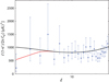 |
Fig. 2. Same as Fig. 1, except magnifying the view at ℓ ≲ 30, where the dominant contribution to |

The calculated angular power Cℓ for Planck-ΛCDM, with kmin = 0, is indicated by the black curve in Figs. 1 and 2, in comparison with the Planck data (blue dots). Our corresponding optimized fit using kmin as a free parameter is represented by the red solid curve. Based on this fit, we find an optimized value
 (7)
(7)
corresponding to a maximum fluctuation size θmax ≈ 127° in the plane of the sky. For a redshift zdec = 1080 at decoupling, this cutoff represents a maximum fluctuation size λmax ∼ 31 Mpc at that redshift. The six basic parameters for this fit, and their confidence regions, are shown in Fig. 3 and listed in Table 1. Note that, in spite of the fact that a kmin compatible with zero appears to be possible within 1σ in the τ − kmin panel of Fig. 3, this is not the case because the 1σ and 2σ regions are different in 1D and 2D. The distinction arises because the 1σ and 2σ levels in the 2D histograms are not the 68% and 95% values used for the 1D distributions. The relevant 1σ and 2σ levels for a 2D histogram of samples are 1 − exp(−0.5)→39.3% and 1 − exp(−2)→86.5%2. Using 39.3% and 86.5% of the region, the contour plots then do exclude a kmin compatible with zero at the 1σ (1D) level.
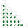 |
Fig. 3. The six basic parameters in ΛCDM. These values are optimized based on the combined data sets SN+DES+BAO+Planck, together with the new parameter (kmin) introduced to represent a cutoff in the primordial power spectrum, 𝒫(k). |
The fact that a non-zero cutoff kmin has minimal, if any, impact on the optimized fit at ℓ ≳ 30, is consistent with the prevailing view that the physical origin of the fluctuations is due to different physical effects above and below ∼1°. It may therefore be useful to compare this optimized value of kmin based on the whole range of ℓ’s with that found when ℓ is restricted to the range (≲30) thought to be dominated by the Sachs-Wolfe effect (Sachs & Wolfe 1967). The optimized parameter values for this case, using the low-ℓ TT data from Planck 2018, combined with the DES, BAO, and Type Ia SNe data sets, are shown in Fig. 4. The corresponding best-fit cutoff kmin for this restricted range is  Mpc−1, consistent with the full-ℓ range value, but even closer to the cutoff found using the angular correlation function. In either case, the cutoff “fixing” the low-power anomaly at ℓ ≲ 4 is fully consistent with the value that completely accounts for the missing correlations at angles ≳60°, suggesting that both of these large-angle anomalies in the standard model are due to the same truncation in 𝒫(k).
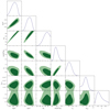 |
Fig. 4. Same as Fig. 3, except now using an optimization of the fit for ℓ ≤ 30, and the low-ℓ TT data from Planck 2018 (Planck Collaboration VI 2020), combined with the DES, BAO, and Type Ia SNe data sets. |
4. Discussion
A side-by-side comparison of the best-fit parameters in ΛCDM with and without a cutoff kmin (Table 1) reveals only negligible differences between them, but the angular power spectrum for ℓ ≲ 4 is improved significantly compared with the data. Thus, the excellent agreement between standard ΛCDM and the CMB data for ℓ ≳ 60 is completely unaffected by our introduction of a cutoff to the primordial power spectrum. Yet, based on the optimized kmin value using the whole ℓ range (and even more so using the restricted range ℓ ≲ 30), we conclude that a zero cutoff is ruled out at a confidence level of ∼2.6σ. On its own, this is already interesting enough for us to study its impact on slow-roll inflation (Liu & Melia 2020; Melia 2020), but when combined with our earlier measurement of kmin based on the angular correlation function (Melia & López-Corredoira 2018), which showed that kmin = 0 was ruled out at a confidence level exceeding 8σ for those data, these two complementary indicators argue compellingly that the primordial power spectrum 𝒫(k) must have been truncated at kmin ∼ 3 × 10⁻⁴ Mpc−1.
These results are completely consistent with the prevailing view that the CMB anisotropies are primarily due to two distinct physical influences: the Sachs-Wolfe effect (Sachs & Wolfe 1967) at small ℓ’s and acoustic oscillations for ℓ ≳ 30. The excellent fit to the data for large ℓ’s (see Fig. 1) reinforces the perception that we understand fairly well the physical process associated with small-angle anisotropies, in spite of the fact that the angular correlation function has been problematic since the beginning (Hinshaw et al. 1996; Bennett et al. 2003; Planck Collaboration VI 2020).
The emerging evidence for a non-zero kmin, on the other hand, speaks directly to the cosmological expansion itself. At ℓ ≲ 30, we see the effects due to the metric perturbations associated with the cosmological dynamics, and therefore the direct influence of the cosmological model itself. In this range, we are probing ever closer to the onset of the hypothesized inflationary expansion, culminating with the cutoff kmin, that signals the very first mode crossing the horizon at the beginning of the quasi-de Sitter phase produced by the inflaton field (Liu & Melia 2020; Melia 2020).
The idea that at least one of the large-angle anomalies may be due to features in the primordial power spectrum, 𝒫(k), has been with us for several decades (see discussion in Planck Collaboration VII 2020). For example, Shafieloo & Souradeep (2004) assumed an exponential cutoff at low k’s, and found an optimized fit of the attenuation generally consistent with the cutoff we have measured in this paper. Their ansatz for 𝒫(k) did not include an actual truncation, however, which would be required for self-consistency with our previous treatment of kmin in Melia & López-Corredoira (2018). The impact on inflation is different in these two cases, since a sharp termination signals a precise time at which inflation would have started. An exponential cutoff is not fully consistent with the notion of horizon-crossing for the freezing of modes. In addition, this early treatment was based on the use of WMAP data (Bennett et al. 2003), whereas our analysis incorporates the higher precision Planck observations (Planck Collaboration VI 2020). In Fig. 4, we have used only the Planck TT data at ℓ ≤ 30, plus other low-redshift data sets, as described in the caption. For Fig. 3, however, we used all of the Planck data, including TT, TE, EE and also both the high-ℓ and other low-redshift data sets. A comparison of these results shows that the optimized value of kmin is very similar in these two cases, suggesting that the other low-redshift data sets, such as DES, BAO and Type Ia SNe, do not significantly affect the limits on the cutoff.
In related work, Nicholson & Contaldi (2009) and Hazra et al. (2014) modeled a “dip” in 𝒫(k) on a scale k ∼ 0.002 Mpc−1 for the WMAP data. Their results confirmed those of an alternative approach (Ichiki et al. 2010), in which an oscillatory modulation was identified around k ∼ 0.009 Mpc−1. These are not a truncation, however, nor are they consistent with our analysis (Melia & López-Corredoira 2018) of a cutoff kmin in the angular correlation function based on the Planck measurements.
Tocchini-Valentini et al. (2005) modeled both a dip at k ∼ 0.035 Mpc−1 and a “bump” at k ∼ 0.05 Mpc−1, also using WMAP data. As with the others, however, these features are not the same as an actual truncation kmin, and our analysis utilizes the latest Planck data, rather than the less precise WMAP measurements. Subsequent work by these authors, notably Tocchini-Valentini et al. (2006), improved on this analysis considerably, though they were still fully reliant on WMAP. These authors found evidence for three features in 𝒫(k), one of which is analogous to our kmin, including a cutoff at ∼0.0001 − 0.001 Mpc−1, with a confidence level of about 2σ. Our analysis based on the improved Planck data produces a tighter constraint on this cutoff, more in line with the kmin found from the angular correlation function. For example, their possible cutoff range exceeds the actual value we have measured for kmin in this paper.
More recently, Hunt & Sarkar (2014, 2015) found evidence in the WMAP data of a cutoff k < 5 × 10⁻⁴ Mpc−1 to 𝒫(k), but concluded that more accurate data, such as those provided by Planck, would need to be used to confirm these results more robustly. The work most closely aligned with our analysis in this paper is that of Iqbal et al. (2015) and Santos da Costa et al. (2018). These two groups arrived at opposite conclusions to each other, however. Though each carried out a thorough analysis of the possible cause for the low CMB power at small ℓ’s, and actually agreed on approximately what value a cutoff (which they called kc, analogous to our kmin) would be needed to address this anomaly, they adopted different model-selection criteria and produced opposing outcomes.
This state of uncertainty has been with us for many years. The approach of Iqbal et al. (2015) and Santos da Costa et al. (2018) was to focus solely on the low-ℓ anomaly and to compare 7 or 8 different models, using a range of model-selection tools. Our approach in this paper has been diametrically opposite to this. We have only one goal in mind, motivated by the physics of inflation. Most importantly, our previous analysis demonstrated that a zero value for kmin is ruled out at over 8σ. Notice, e.g., how different this outcome is compared to that of Santos da Costa et al. (2018), who concluded that standard inflationary cosmology, without any adjustment to 𝒫(k), is preferred by the CMB data and their choice of model selection criteria.
The work we have carried out in this paper is based on the conclusion of our previous work suggesting that only a simple cutoff kmin in 𝒫(k) is well motivated by the CMB angular correlation function. We have not compared different models, nor have we based our analysis on a subjective choice of model selection criteria, which seem to produce the divergent outcomes seen, e.g., in Iqbal et al. (2015) and Santos da Costa et al. (2018).
We showed in Liu & Melia (2020) that the cutoff kmin measured via the CMB angular correlation function apparently rules out all inflationary models based on slow-roll potentials, including those that may have been preceded by radiation-dominated and/or kinetic-dominated phases (see also Handley et al. 2014). With such a cutoff, inflation could not simultaneously have solved the horizon problem and accounted for the observed CMB fluctuation spectrum. This is the reason why a confirmation of kmin based on the angular power spectrum is so essential. The two large-angle anomalies are not necessarily related (see also Planck Collaboration VII 2020), so our previous result with kmin does not by itself ensure that it is also consistent with the much better studied angular power spectrum, nor that it can also mitigate the missing power at low-ℓ’s. This paper has therefore been highly focused on these two issues alone. Nevertheless, the fact that our measured value of kmin is consistent with that found by Iqbal et al. (2015) and Santos da Costa et al. (2018) is crucial because it demonstrates a consistent outcome by three different groups.
We mention in passing that an extension of the work reported by Iqbal et al. (2015) and Santos da Costa et al. (2018) to include the angular correlation function would be very beneficial. Our previous assessment was that only a simple cutoff in 𝒫(k) could completely account for the missing correlations at large angles. It would be interesting to see if an independent examination of these data, using a range of other models with various model selection tools, such as those explored by these two groups, could alter this conclusion.
In this paper, we have met our primary goal of showing that the introduction of a non-zero cutoff in 𝒫(k) does not at all affect the excellent agreement between the predictions of ΛCDM and the CMB angular power spectrum at ℓ ≳ 30. This is critical because it is widely believed that the origin of the CMB anisotropies in this domain is well understood, given that it relies on well-established astrophysical principles.
We have also demonstrated that the origin of the missing power in the low-ℓ multipoles, particularly at ℓ = 2 − 5, is very likely due to the same physical influence impacting the missing correlations at large angles. The two optimized values of kmin, i.e., (3.14 ± 0.36)×10−4 Mpc−1 for the latter, and  Mpc−1 for the former, are fully consistent with each other. These complementary results reinforce the view that we are beginning to see direct evidence of the initiation of inflation, if this process actually did occur. Nevertheless, the disparity between the primordial fluctuation spectrum expected under these conditions and what is actually required to produce the CMB anisotropies, increases the tension between the concordance model and the observations.
5. Conclusion
The existence of large-angle anomalies in the temperature is uncontested though, given the modest significance with which they disagree with the standard model, and the fact that they were detected a posteriori, makes it unclear how much evidence they actually provide for a true, physical origin (Planck Collaboration VII 2020). They may simply be statistical fluctuations, even though such an outcome appears to be highly unlikely. Nevertheless, if any of them do indeed correspond to a real physical effect, it would be extremely important for us to confirm this, justifying the continued attention paid to these unusual features.
As noted earlier, however, we must still temper our conclusions regarding the reality of these large-angle anomalies, given that the Planck Collaboration VII (2020) study found only weaker evidence for them in the polarization data. This is why upcoming missions designed specifically to measure the CMB polarization will be so critical to the continuation of this work. For example, LiteBIRD has been selected for development and launch in 2028 by the Japan Aerospace Exploration Agency, with the goal of mapping the CMB polarization over the whole sky with unprecedented precision (Hazumi et al. 2019). Its required angular coverage will correspond to 2 ≤ ℓ ≤ 200, perfectly attuned to the requirements for the analysis in this paper.
Perhaps even more impressively, the Probe of Inflation and Cosmic Origins (PICO) mission (Hanany et al. 2019) is still in the study phase, but is projected to be an imaging polarimeter scanning the sky for 5 years in 21 frequency bands spread between 21 and 799 GHz. If selected, PICO will produce a full-sky survey of the intensity and polarization of the CMB with a final combined-map noise level equivalent to an amazing 3300 Planck missions.
And as a prominent third example, the Cosmic Origins Explorer (CORE) mission (Delabrouille et al. 2018) proposed to the European Space Agency is projected to have 19 frequency channels spanning the 60 − 600 GHz range, and an angular resolution from 2′ to 18′. It will observe the entire sky repeatedly over four years of continuous scanning. Its design will be optimized for complementarity with ground-based observations, performing observations–such as that required by the analysis carried out in this paper–essential to CMB polarization science not achievable without a dedicated space mission.
Proposed, or in-progress, experiments to map the CMB polarization from the ground include the Simons Observatory (Ade 2019), located in the high Atacama Desert in Northern Chile inside the Chajnator Science Preserve, at an altitude of 5200 meters. Though its goals are currently not as lofty as those of the space-based missions, its principal aim is to produce a polarization map of the sky with an order of magnitude better sensitivity than Planck.
The principal aim of all these future missions is, of course, to detect the B-mode polarization in the tell-tale signature of gravity waves generated during inflation. Nevertheless, a more precise measurement of the E-mode polarization anisotropies at a much higher sensitivity than that available to Planck should answer the question of whether or not the large-angle anomalies seen in the temperature are also confirmed in the polarization maps. This would then provide compelling evidence that they are not merely due to secondary, background or instrumental effects, further motivating a study of the impact on inflationary theory of a cutoff, kmin, in the primordial power spectrum, 𝒫(k).
For example, as shown by Liu & Melia (2020), a kmin like that measured earlier in our analysis of the angular correlation function (Melia & López-Corredoira 2018), and reinforced by the work reported in this paper, which is based exclusively on the angular power spectrum, rules out the majority – if not all – of the slow-roll inflaton potentials proposed thus far. If one insists on inflation simultaneously fixing the horizon problem and accounting for the observed primordial power spectrum, 𝒫(k), then the accelerated expansion resulting from these hypothesized fields misses the required comoving distance by a factor ∼10. Moreover, neither a radiation-dominated, nor a kinetic-dominated, phase preceding inflation can alleviate this disparity (Liu & Melia 2020; see also Handley et al. 2014).
Our results reinforce the growing view that, at a minimum, inflation probably needs to be modified or, at worst, needs to be replaced, in order to conform with these observations.
Acknowledgments
We are grateful to the anonymous referee for their helpful and thoughtful review of this manuscript. FM is also grateful to Amherst College for its support through a John Woodruff Simpson Lectureship. This work is partially supported by the National Natural Science Foundation of China (grant No. U1831122), the Youth Innovation Promotion Association (2017366), and the Key Research Program of Frontier Sciences (grant No. ZDBS-LY-7014) of Chinese Academy of Sciences, at Purple Mountain Observatory, and by the Innovation and Entrepreneurial Project of Guizhou Province for High-level Overseas Talents (grant No. 2019-02), the National Natural Science Foundation of China (grant No. 11903010), and the Science and Technology Fund of Guizhou Province (grant No. 2020-1Y020), at Guizhou Normal University.
References
- Abbott, T. M. C., Abdalla, F. B., Alarcon, A., et al. 2018, Phys. Rev. D, 98, 056 [CrossRef] [Google Scholar]
- Ade, P., Aguirre, J., Ahmed, Z., et al. 2019, JCAP, 02, 056 [CrossRef] [Google Scholar]
- Alam, S., Ata, M., Bailey, S., et al. 2017, MNRAS, 470, 2617 [Google Scholar]
- Barrau, A., Cailleteau, T., Grain, J., & Mielczarek, J. 2014, Class. Quant. Grav., 31, 053001 [CrossRef] [Google Scholar]
- Bennett, C. L., Hill, R. S., Hinshaw, G., et al. 2003, ApJS, 148, 97 [Google Scholar]
- Bennett, C. L., Hill, R. S., Hinshaw, G., et al. 2011, ApJS, 192, 17 [NASA ADS] [CrossRef] [Google Scholar]
- Berera, A., Fang, L. Z., & Hinshaw, G. 1998, Phys. Rev. D, 57, 2207 [NASA ADS] [CrossRef] [Google Scholar]
- Boyanovsky, D., de Vega, H. J., & Sanchez, N. G. 2006, Phys. Rev. D, 74, 123007 [NASA ADS] [CrossRef] [Google Scholar]
- Broy, B. J., Roest, D., & Westphal, A. 2015, Phys. Rev. D, 91, 023514 [NASA ADS] [CrossRef] [Google Scholar]
- Campanelli, L., Cea, P., & Tedesco, L. 2006, Phys. Rev. Lett., 97, 131302 [NASA ADS] [CrossRef] [Google Scholar]
- Campanelli, L., Cea, P., & Tedesco, L. 2007, Phys. Rev. D, 76, 063007 [NASA ADS] [CrossRef] [Google Scholar]
- Cicoli, M., Downes, S., Dutta, B., Pedro, F. G., & Westphal, A. 2014, JCAP, 2014, 030 [Google Scholar]
- Contaldi, C. R., Peloso, M., Kofman, L., & Linde, A. 2003, JCAP, 2003, 002 [Google Scholar]
- Copi, C. J., Huterer, D., Schwarz, D. J., & Starkman, G. D. 2009, MNRAS, 399, 295 [NASA ADS] [CrossRef] [Google Scholar]
- Copi, C. J., Huterer, D., Schwarz, D. J., & Starkman, G. D. 2010, Adv. Astron., 2010, 847541 [CrossRef] [Google Scholar]
- Copi, C. J., Huterer, D., Schwarz, D. J., & Starkman, G. D. 2015, MNRAS, 451, 2978 [CrossRef] [Google Scholar]
- Das, S., & Souradeep, T. 2014, JCAP, 02, 002 [Google Scholar]
- Das, S., Goswami, G., Prasad, J., & Rangarajan, R. 2015, JCAP, 06, 001 [NASA ADS] [Google Scholar]
- Delabrouille, J., de Bernardis, P., Bouchet, F. R., et al. 2018, JCAP, 04, 014 [CrossRef] [Google Scholar]
- Efstathiou, G. 2003a, MNRAS, 343, L95 [Google Scholar]
- Efstathiou, G. 2003b, MNRAS, 346, L26 [NASA ADS] [CrossRef] [Google Scholar]
- Hajian, A., & Souradeep, T. 2003, ApJ, 597, L5 [NASA ADS] [CrossRef] [Google Scholar]
- Hanany, S., Alvarez, M., Artis, E., et al. 2019, ArXiv e-prints [arXiv:1902.10541] [Google Scholar]
- Handley, W. J., Brechet, S. D., Lasenby, A. N., & Hobson, M. P. 2014, Phys. Rev. D, 89, 063505 [NASA ADS] [CrossRef] [Google Scholar]
- Hazra, D. K., Shafieloo, A., & Souradeep, T. 2014, JCAP, 11, 011 [Google Scholar]
- Hazumi, M., Ade, P. A., Akiba, Y., et al. 2019, J. Low Temp. Phys., 194, 443 [NASA ADS] [CrossRef] [Google Scholar]
- Hinshaw, G., Branday, A. J., Bennett, C. L., et al. 1996, ApJ, 464, L25 [Google Scholar]
- Hunt, P., & Sarkar, S. 2014, JCAP, 01, 025 [Google Scholar]
- Hunt, P., & Sarkar, S. 2015, JCAP, 01, 052 [CrossRef] [Google Scholar]
- Ichiki, K., Nagata, R., & Yokoyama, J. 2010, Phys. Rev. D, 81, 083010 [NASA ADS] [CrossRef] [Google Scholar]
- Iqbal, A., Prasad, J., Souradeep, T., & Malik, M. A. 2015, JCAP, 06, 014 [Google Scholar]
- Lewis, A., & Bridle, S. 2002, Phys. Rev. D, 66, 103511 [Google Scholar]
- Lewis, A., Challinor, A., & Lasenby, A. 2000, ApJ, 538, 473 [Google Scholar]
- Liu, J., & Melia, F. 2020, Proc. R. Soc. A, 476, 20200364 [NASA ADS] [CrossRef] [Google Scholar]
- Luminet, J. P., Weeks, J. R., Riazuelo, A., Lehoucq, R., & Uzan, J. P. 2003, Nature, 425, 593 [NASA ADS] [CrossRef] [Google Scholar]
- Martin, J., Ringeval, C., & Vennin, V. 2013, JCAP, 06, 021 [CrossRef] [Google Scholar]
- Melia, F. 2018, EPJC, 78, 739 [NASA ADS] [CrossRef] [EDP Sciences] [Google Scholar]
- Melia, F. 2020, The Cosmic Spacetime (Taylor& Francis: Oxford) [CrossRef] [Google Scholar]
- Melia, F., & López-Corredoira, M. 2018, A&A, 610, A87 [NASA ADS] [CrossRef] [EDP Sciences] [Google Scholar]
- Nicholson, G., & Contaldi, C. R. 2009, JCAP, 07, 011 [Google Scholar]
- O’Dwyer, I. J., Eriksen, H. K., Wandelt, B. D., et al. 2004, ApJ, 617, L99 [CrossRef] [Google Scholar]
- Planck Collaboration VI. 2020, A&A, 641, A6 [NASA ADS] [CrossRef] [EDP Sciences] [Google Scholar]
- Planck Collaboration VII. 2020, A&A, 641, A7 [NASA ADS] [CrossRef] [EDP Sciences] [Google Scholar]
- Planck Collaboration XXI. 2016, A&A, 594, A21 [NASA ADS] [CrossRef] [EDP Sciences] [Google Scholar]
- Planck Collaboration XXIV. 2014, A&A, 571, A24 [NASA ADS] [CrossRef] [EDP Sciences] [Google Scholar]
- Powell, B. A., & Kinney, W. H. 2007, Phys. Rev. D, 76, 063512 [NASA ADS] [CrossRef] [Google Scholar]
- Sachs, R. K., & Wolfe, A. M. 1967, ApJ, 147, 73 [NASA ADS] [CrossRef] [Google Scholar]
- Santos da Costa, S., Benetti, M., & Alcaniz, J. 2018, JCAP, 03, 004 [Google Scholar]
- Scardigli, F., Gruber, C., & Chen, P. 2011, Phys. Rev. D, 83, 063507 [NASA ADS] [CrossRef] [Google Scholar]
- Scolnic, D. M., Jones, D. O., Rest, A., et al. 2018, ApJ, 859, 101 [NASA ADS] [CrossRef] [Google Scholar]
- Seljak, U., & Zaldarriaga, M. 1996, ApJ, 469, 437 [NASA ADS] [CrossRef] [Google Scholar]
- Shafieloo, A., & Souradeep, T. 2004, Phys. Rev. D, 70, 043523 [NASA ADS] [CrossRef] [Google Scholar]
- Tocchini-Valentini, D., Douspis, M., & Silk, J. 2005, MNRAS, 359, 31 [NASA ADS] [CrossRef] [Google Scholar]
- Tocchini-Valentini, D., Hoffman, Y., & Silk, J. 2006, MNRAS, 367, 1095 [NASA ADS] [CrossRef] [Google Scholar]
- Troxel, M. A., MacCrann, N., Zuntz, J., et al. 2018, Phys. Rev. D, 98, 043528 [Google Scholar]
- Wang, I. C., & Ng, K. W. 2008, Phys. Rev. D, 77, 083501 [NASA ADS] [CrossRef] [Google Scholar]
- Wright, E. L., Bennett, C. L., Gorski, K., Hinshaw, G., & Smoot, G. F. 1996, ApJ, 464, L21 [Google Scholar]
All Tables
All Figures
|
Fig. 1. Angular power spectrum (blue dots) estimated with the NLIC method, with 1σ Fisher errors. These error bars include cosmic variance, approximated as Gaussian (see Fig. 1 in Planck Collaboration VI 2020). The ΛCDM best fit model ( |
| In the text | |
|
Fig. 2. Same as Fig. 1, except magnifying the view at ℓ ≲ 30, where the dominant contribution to |
| In the text | |
|
Fig. 3. The six basic parameters in ΛCDM. These values are optimized based on the combined data sets SN+DES+BAO+Planck, together with the new parameter (kmin) introduced to represent a cutoff in the primordial power spectrum, 𝒫(k). |
| In the text | |
|
Fig. 4. Same as Fig. 3, except now using an optimization of the fit for ℓ ≤ 30, and the low-ℓ TT data from Planck 2018 (Planck Collaboration VI 2020), combined with the DES, BAO, and Type Ia SNe data sets. |
| In the text | |
Current usage metrics show cumulative count of Article Views (full-text article views including HTML views, PDF and ePub downloads, according to the available data) and Abstracts Views on Vision4Press platform.
Data correspond to usage on the plateform after 2015. The current usage metrics is available 48-96 hours after online publication and is updated daily on week days.
Initial download of the metrics may take a while.