| Issue |
A&A
Volume 655, November 2021
|
|
|---|---|---|
| Article Number | A14 | |
| Number of page(s) | 9 | |
| Section | Planets and planetary systems | |
| DOI | https://doi.org/10.1051/0004-6361/202140365 | |
| Published online | 28 October 2021 | |
Asteroid pairs: method validation and new candidates
Institute of Astronomy, V. N. Karazin Kharkiv National University,
35 Sumska Str.,
Kharkiv
61022,
Ukraine
e-mail: This email address is being protected from spambots. You need JavaScript enabled to view it.
Received:
15
January
2021
Accepted:
17
July
2021
Abstract
Context. An asteroid pair can be described as two asteroids with very similar heliocentric orbits that are genetically related but not gravitationally bound. They can be produced by asteroid collisions or rotational fission. Although over 200 asteroid pairs are known, many more remain to be identified, especially among the newly discovered asteroids.
Aims. The purpose of our work is to find new asteroid pairs in the inner part of the main belt with a new pipeline for asteroid pair search, and to validate the pipeline on a sample of known asteroid pairs.
Methods. Initially, we selected pair candidates in the five-dimensional space of osculating orbital elements. Then the candidates were confirmed using numerical modeling with the backtrack integration of their orbits, including the perturbations from the largest main-belt asteroids and the influence of the non-gravitational Yarkovsky effect.
Results. We performed a survey of the inner part of the main belt and found ten new probable asteroid pairs. Their estimated formation ages lie between 30 and 400 kyr. In addition, our pipeline was tested on a sample of 17 known pairs, and our age estimates agree with those indicated in the literature in most of the cases.
Key words: minor planets, asteroids: general / celestial mechanics
© ESO 2021
1 Introduction
In the past few decades many asteroid pairs, two asteroids with similar heliocentric orbits that are genetically related but not gravitationally bound, have been found among the main-belt asteroids, whose members have very similar orbits and share a common origin.
There are two major ways of how a pair is created. First, a collision of two asteroids can shatter them into fragments (Michel et al. 2015). Second, a rapidly rotating asteroid can undergo rotational fission (Scheeres 2007; Vokrouhlický et al. 2015) due to centrifugal forces. The rapid rotation can be caused by the YORP effect (Yarkovsky–O’Keefe–Radzievskii–Paddack effect), which is the radiation pressure torque acting on an asteroid of an asymmetric shape. One possible outcome of such rotational fission is the decay of an asteroid into several gravitationally unbound fragments (Jacobson & Scheeres 2011). Both collisional disruption and rotational fission can create clusters with multiple members of different sizes (Pravec et al. 2018). In this article we do not look for such clusters, but merely for pairs. This leaves open the possibility that some of the pairs we find could in fact be some of the largest members of certain clusters.
The two members of a newly formed asteroid pair initially have a small relative distance and velocity. Over time their orbits drift apart due to perturbations from planets, and to a lesser extent due to the non-gravitational Yarkovsky effect. Even if the components of the pair are no longer bound gravitationally, their relation can be discovered via various methods. Thus, the task is to identify such a pair and to uncover its dynamic history.
One of the first successful attempts to discover asteroid pairs was made in Vokrouhlický & Nesvorný (2008), where pair candidates were pre-selected based on their proximity in the five-dimensional space of osculating orbital elements, and then confirmed by the orbital integration. After that, a number of dynamical studies were published (Pravec & Vokrouhlický 2009; Pravec et al. 2019) that massively expanded the list of identified pairs. Other studies have shown the necessity of taking into account the most massive perturbers of the main belt (Ceres, Vesta, Pallas) in numerical calculations of the formation age of pairs (Galád 2012). At the same time, the findings by Vokrouhlický & Nesvorný (2008) and Žižka et al. (2016) opened the road to the identification of very young asteroid pairs. Recent advancements in numerical propagation software (Rein & Liu 2012), the main instrument in asteroid pairs identification, made it easier to contribute to the search for asteroid pairs.
We began our work in asteroid pair search with the development of a comprehensive software pipeline, both for the identification and verification of pair candidates. We chose the inner part of the main belt (2.0–2.5 au) as the area of our search. The density of discovered asteroids is the highest in this region, which increases the chances of finding an asteroid pair. Moreover, the high collision rates and short YORP timescales guarantee a high pair production rate.
We present the first results of our survey in this paper. Section 2 describes the methods of asteroid pair search and verification that were used in this article. Section 3 covers the results, specifically ten newly identified probable asteroid pairs, whereas Sect. 4 describes the outcome of this work in general, along with our further plans.
2 Research methodology
2.1 Initial pair search in five-dimensional space
To identify asteroids as a potential pair, we use a modified five-dimensional version (Vokrouhlický & Nesvorný 2008) of the three-dimensional metric by Zappalà (1990), who applied it to asteroid families via the hierarchical clustering method (HCM). In contrast to the search for asteroid families, where HCM is used with proper orbital elements of the asteroids, we use osculating orbital elements for our search. The point is that typical asteroid families are old enough to have erased any initial grouping in the phase space of the osculating elements, whereas the pairs we are searching for are sufficiently young to still retain the close resemblance even in the osculating elements. The main advantage of using the osculating orbital elements is that the longitude of the ascending node and the argument of perihelion preserve additional information about the orbit similarity. This reduces the number of false pair candidates, which would inevitably appear while using only the proper elements of the asteroids. As was shown in Nesvorný & Vokrouhlický (2006), this approach allows us to reliably recover pairs with formation times that are ≲1 million years. The method consists of calculating the distance d between asteroids in the five-dimensional space of the Keplerian orbital elements using the following formula:
 (1)
(1)
Here the semi-major axis a, the eccentricity e, the inclination i, the longitude of the ascending node Ω, and the longitude of perihelion ϖ are the Keplerian elements, (δa, δe, δ sin i, δϖ, δΩ) is the separation vector of neighboring bodies in the phase space, n is the mean motion of the asteroid. Following Nesvorný & Vokrouhlický (2006), we adopted the next values of the coefficients for our computations: ka = 5∕4, ke = ki = 2, and  .
.
The smaller the phase distance between given asteroids, the more similar their orbits, and it is more likely that such a combination of asteroids may turn out to be evolutionarily related and gravitationally bound in the past. In our search we limited the cutoff distance in the phase space to d = 100 m s−1. On the one hand, for larger phase distances young asteroid pairs are less probable, on the other hand, it is larger than the value that is commonly used (Pravec et al. 2019), which gives us the opportunity to find new pair candidates in well-studied regions.
For our calculations we used the osculating orbital elements provided by the JPL Horizons system1. The values of orbital elements are given for the same epoch. The phase distances for potential pairs were also calculated for several MPC databases2 covering the years 2004–2019, and then the median value of the phase distance was calculated. This potentially makes our calculation less susceptible to errors of individual databases and short-term perturbations. In total, 15 MPC databases were used, which are mostly equidistant in time. As a result, ~ 500 potential pairs were found with a median distance of up to 100 m s−1 in the phasespace.
Since the pair candidates we found also contain confirmed pairs, we cross-matched the obtained pair candidates with the known pairsin order not to waste the resources on their simulation. To do this, we used the Johnston database of known pairs (Johnston 2020) as well as small catalogs from Pravec et al. (2019). Out of over 500 pair candidates found, 67 were identified as the known ones, which represent more than 90 percent (67/72) of the known pairs listed in the Johnston database. Since the list of known pairs is constantly being updated, each studied pair is checked by NASA ADS3 for related articles. Pair candidates that were not mentioned in any source were selected for further processing.
2.2 Numerical modeling
For further verification of the obtained potential pairs, we use numerical modeling. The principle of verification is to use backtrack integration for the components of the pair to find their close approaches, which are characterized by the small relative velocities and distances. For numerical modeling, we use the REBOUND package, which is available for the Python and C programming languages (Rein & Liu 2012). The REBOUND package provides a variety of N-body integrators, of which we used WHFast, SABA, and IAS15. The WHFast and SABA integrators (Rein & Tamayo 2015) were applied primarily for the pairs with unambiguous and unique encounters, whereas IAS15 (Rein & Spiegel 2015) was used for pairs with more complex dynamical behavior. Although IAS15 is distinctly slower, its high-order nature with the adaptive integration time step gives optimal results down to machine precision for errors associated with numerical integration. The length of the time step used in integrations is 1–3.65 days for WHFast and SABA integrators, whereas the IAS15 minimal time step was limited to 0.5 days. The time step was chosen for each pair individually, depending on the radius of the Hill sphere of the largest component of the pair and the mutual velocity of the clones during the encounters.
As a frame for computations we built a model that consists of all the planets in the Solar System. The most massive bodies of the main belt, which are Ceres, Vesta, and Pallas, were also taken into account. These bodies, in addition to the planets, are the principal main-belt perturbers, and can significantly influence the behavior of asteroids, thus modifying the determined age of the pair (Galád 2012). Planets with moons are represented by their barycenters.
Since the orbital elements of asteroids are known with some uncertainty, which is associated with the accuracy of observations, it is necessary to take into account these errors when adding asteroids to the simulation. To implement this we generate an array of asteroid clones with the values of orbital elements within the given accuracy. The orbital elements, and their uncertainties, were taken from the JPL Horizons system. To consider the possible correlation between orbital parameters, we incorporated the mechanism for the creation of asteroid clones that was proposed in Vokrouhlický et al. (2017). The initial orbital elements of the clones E are determined as
 (2)
(2)
where z is the six-dimensional vector whose components are random deviates of the normal distribution, and E* is the best-fit solution. The covariance matrix T is obtained using the Cholesky decomposition method and satisfies TTT = Σ, where Σ is the normal matrix. JPL Horizons is not always able to provide covariance matrices and osculating orbital elements for the same epoch. To overcome this, clones of the asteroids are added to the simulation at their corresponding epochs as the integration into the past progresses.
For an accurate calculation of the pair’s evolution, especially in close approaches, it is important to take into account the mutual gravitational interaction of the two components. While simulating clones with masses makes it impossible to simulate more than two clones for a pair in one integration, it could give more robust results where multiple encounters occur. To do so it is necessary to take into account the mass of asteroids. Since the mass for many asteroids is poorly constrained, in the first approximation the mass can be derived from the asteroid radius R and bulk density ρ using the formula
 (3)
(3)
where the bulk density is assumed to be 2 × 10³ kg m−3 if not provided by the HORIZONS system. For asteroids whose radius is unknown, the radius is calculated using the asteroid’s absolute magnitude H and geometric albedo pv using the following formula (Harris & Harris 1997):
![Mathematical equation: \begin{equation*}R_{\textrm{ast}} = \frac{1329}{2\sqrt{p_v}}10^{-0.2H} [\mathrm{km}].\end{equation*}](/articles/aa/full_html/2021/11/aa40365-21/aa40365-21-eq5.png) (4)
(4)
Mass is also required to calculate the Hill sphere radius and the escape velocity; both of these parameters are used in the criteria for close approaches.
The Hill sphere radius, the distance to which the body dominates in the gravitational attraction, can be calculated using the equation
![Mathematical equation: \begin{equation*}R_{\textrm{Hill}} = a\sqrt[3]{\frac{{m}}{3M}},\end{equation*}](/articles/aa/full_html/2021/11/aa40365-21/aa40365-21-eq6.png) (5)
(5)
where a and m are the semi-major axis and the mass of the primary component of the pair, and M is the mass of the Sun.
The escape velocity is the minimum speed needed to escape from the gravitational influence of a given body. Given the mass m of the primary component and the distance r between the center of mass of the primary and the secondary, the escape velocity is calculated as
 (6)
(6)
We are mainly interested in those simulations in which close encounters between the components of a pair occur. We define such encounters by the limits of 5 RHill and 2ve for the component with the largest mass (Pravec et al. 2019). For pair candidates with worse convergence, these conditions are extended up to 10–20 RHill and 4–8 ve (Pravec et al. 2019).
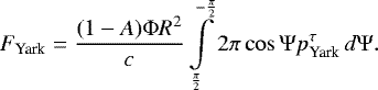
The simulation also needs to take into account the Yarkovsky effect, which is a non-gravitational force arising due to non-isotropic thermal radiation from a rotating asteroid heated by the Sun. The result of the Yarkovsky effect can lead to the drift of the semi-major axis of the asteroid, either towards its increase for prograde rotators, or decrease in the case of retrograde rotators. This effect can strongly modify the behavior of an asteroid pair and make changes to its determined age. Since the physical and orbital parameters of an asteroid are often not very precise, the simplified formula for the Yarkovsky effect is sufficient. Using Eq. (41) from Golubov et al. (2016) and integrating the pressure over the surface of an approximately spherical asteroid, we get the following expression for the Yarkovsky force (see Appendix A for derivation):
 (7)
(7)
Here R is the radius of the asteroid, c is the speed of light,  is the solar constant at the asteroid’s orbit, Φ0 is the solar constant at a0 = 1 AU, and a is the semi-major axis of the asteroid’s orbit.
To determine the direction of this force, it is also necessary to know the direction of rotation of the asteroid around its axis, which is also mostly unknown. For this reason, for each clone we generate a random value of the Yarkovsky force which amounts to Eq. (7) multiplied by constant with uniform distribution in the range [−1, 1]. The YORP effect is not taken into account in this work, since we are looking for pairs of age ≤1 Myr, which is much less than the typical YORP timescales (Golubov & Scheeres 2019).
Although our aim is to find asteroid pairs with ages up to 1 million years, many of the pairs under consideration are much younger. Thus, to save computation time the reasonable choice is to limit the integration time to the latest possible encounter individually for every pair. In order to do this we checked the relative distances and velocities for a sample of one thousand clones to determine time limits that would cover all the possible encounter times within 1 Myr interval. Then, having found these moments, we integrated 10–30 thousand clones in the obtained time intervals, including more clones for pairs with a worse convergence to compensate for larger dispersion.
To check the efficacy and accuracy of our pipeline we compared its output with the results published in the literature. We took a sample of pairs with known formation ages, which were re-discovered in our survey, and recalculated their formation times. The comparison of our results and the results of other authors are shown in Fig. 1 and Table 1. The quite good agreement of our result with the previous studies corroborates that our pipeline canbe used to reliably discover pairs and to obtain their ages. The results are mostly within the known limits, although the errors can deviate from the values cited in the literature for pairs with ambiguous multiple encounters.
3 Results
Taking into consideration that the pipeline works correctly, we continued our search and found a number of pairs that satisfy the condition of close encounters during numerous backtrack integrations.
Following Pravec & Vokrouhlický (2009), we checked the background around the obtained pairs for uniformity of its distribution and calculated the statistical significance of the pairs. We adopted thethreshold values for the probability of a number of orbits surrounding the specific pair P1∕2, to be 0.01 for pairs with d < 10 m s−1, and 0.05 for pairs with greater d. Pairs with greater P1∕2 pass the test on the uniform distribution.The ratio P2∕Np gives the probability of orbital coincidence of two genetically unrelated asteroids; a pair is considered to be statistically significant if P2 ∕Np ≪ 1 Some contamination by coincidental pairs is expected with P2∕Np = 0.1 and larger. Orbital elements for the selected pairs are presented in Table 2, and results on estimated age formation together with significance estimates are in Table 3.
Using the new database of SDSS colors for moving objects (Sergeyev & Carry 2021), we were able to obtain the color indices for eight asteroids, with four of them being members of two pairs, allowing us to estimate the feasibility ofpairs not only with the orbital, but also with the optical properties. This can be done using color indices a* and i − z (Ivezić et al. 2001), or a* and albedo (Slyusarev 2020), with a* defined as
 (8)
(8)
Here g, r, and i are the magnitudes in the corresponding SDSS filters. The more similar the parameters a* and (i − z) for the components of the pair, the more likely they are to be of the same spectral type.
While no information was found on spectral classes or color indices for the remaining pair candidates, we can baseour calculations on the assumption that the components of the pair tend to be of the same spectral type, thus of the same albedo (if not provided by JPL HORIZONS system). With the available information on absolute magnitudes, we can roughly estimate size ratios for the components of the pair.
We use the residual velocity and coordinate differences to make a preliminary guess of how the pair was created. A good convergence of coordinates and velocities simultaneously might be a manifestation of a pair formation via the YORP fission, whereas a relatively large velocity difference can imply a collisional scenario. In some cases, especially for older pairs, improved orbit determination with the robust Yarkovsky effect will be needed to obtain more reliable results.
In the following paragraphs, we describe each pair candidate listed in order of determined age, whereas in Figs. 2 and 3 we plot the distribution of their estimated formation times.
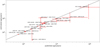 |
Fig. 1 Age comparison between our pipeline and the literature. The x-axis of the plot shows the formation times of these pairs taken from the literature, and the y-axis shows the corresponding times calculated by our program. The red lines are the error bars for both cases. The black dashed line represents the case when both results are in perfect agreement. |
Osculating orbital elements of the pair candidates for epoch MJD 59000.5.
Main data on new pair candidates.
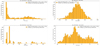 |
Fig. 2 Estimated formation times for the discovered asteroid pair candidates. These distributions include only the clones that had close encounters within the specified vesc and RHill limits. The limits are shown in the legend of each figure. |
271685 (2004 RF90) – 2003 UT336
Asteroid 271685 (2004 RF90) is the primary of the pair with 17.1 mag, and 2003 UT336 is 18.8 mag, with adiameter ratio of 1:2.2. A total of 7% of the clones satisfy the encounter conditions, with multiple encounters for each clone, the closest of which happened 28.1 K yr ago. Interestingly, the distribution has one prominent peak with episodic close encounters following it. The low encounter velocities venc ~ vesc, and renc ≤ 5rHill for this pair indicate that it can be a result of the rotational disruption due to the YORP effect. Using Eq. (8), a* for the components was estimated. 2003 UT336 has a* = 0.18 ± 0.13 and 2004 RF90 has a* = 0.16 ± 0.07. While having high uncertainties, this result indicates that the components could be of the same spectral type, and increases the probability that this pair is a real one.
30243 (2000 HS9) – 2015 DF67
The components have absolute magnitudes of 16.0 mag for 2000 HS9, and 19.2 mag for 2015 DF67, with the diameter ratio of 1:4.3. It has a good convergence with 10% of clones that satisfy the close encounter conditions, with multiple encounters. It has one well-determined peak with a small spread, possibly a result of disruption due to the YORP effect. Components 2000 HS9 and 2015 DF67 have a* values of a* = 0.10 ± 0.04 and a* = −0.09 ± 0.25, respectively. The value for the secondary component agrees with the primary within its error bars, but is not constrained enough to make any strong conclusions based on optical properties.
405222 (2003 RV20) – 2010 TH35
Asteroid 405222 (2003 RV20) is the primary with 17.7 mag, and 2010 TH35 has 18.6 mag, with a diameter ratio of 1:1.5. This pair has a good convergence within 2vesc and 5 RHill limits with 10% of encounters. Most clones are grouped at the age of 48 kyr with multiple smaller peaks of encounters following up to 160 kyr age. The pair is possibly a result of disruption due to the YORP effect.
80245 (1999 WM4) – 540161 (2017 QD23)
Asteroid 1999 WM4 is the primary with 15.6 mag, and 2017 QD23 is the secondary component with 18.3 mag, implying a diameter ratio of 1:3.5. The resulting encounters are spread around 65 K–75 kyr years region, with 15% of the encounters within 2vesc and 5 RHill limits. The test for a uniform background asteroid distribution shows that the pair has P1∕2 = 0.08, which is close to the threshold value of 0.05. Therefore, the pair 1999 WM4 – 2017 QD23 is located in a region with some overdensity, and potentially may be part of a bigger structure like a small family or a cluster. It also has a high P2 ∕Np ratio, which indicates that it can be a coincidental pair, but the results of numerical integration suggest that the members of this pair had close orbital evolution and could be genetically related.
204655 (2006 BJ193) – 2017 FE106
Asteroid 204655 2006 BJ193 is the primary component of this pair with the absolute magnitude of 17.5 mag, while 2017 FE106 is smaller, with only 19.3 mag. The diameter ratio is 1:2.1. The pair has high median values for the encounter velocity, which is 30 times higher than the estimation for the escape velocity of the primary, and medium relative distances, implying that it might be a collisional pair. Only 0.9% of the clones satisfy the encounter conditions.
95251 (2002 CR55) – 2015 VP32
Asteroid 2015 VP32 has 18.7 mag, while the primary 2002 CR55 has H = 15.9 mag, resulting in the diameter ratio 1:3.6. The clones converge in 1.5% of cases, and the encounters are scattered within the 10 RHill, 6vesc margin.
 |
Fig. 3 Distribution of estimated formation times for the discovered asteroid pair candidates. Continuation of Fig. 2. |
2015 XO12 – 524324 (2001 WY4)
The primary 2015 XO12 has 17.8 mag, and the secondary 524324 (2001 WY4) has H = 18.4 mag. The diameter ratio is 1:1.3. The encounters are closely grouped in time. Their relative distance is within eight times the radius of the Hill sphere, and their relative velocity is ten times the estimated escape velocity of 2015 XO12. A total of 3.5% of integrations lead to encounters. The pair is possibly the result of a collisional disruption.
13001 Woodney (1981 VL) – 531931 (2013 CX44)
Asteroid 13001 Woodney (1981 VL) has H = 14.4 mag, and the secondary component is 2013 CX44, with a magnitude of 17.9 mag. These magnitudes translate into a 1:5 ratio for the diameters. This is one of the oldest pairs in our sample, with 5% of clones having multiple encounters scattered along a large time range in the vicinity of 2.5 × 10⁵ yr within 10 RHill, 4vesc margins.
45223 (1999 XF200) – 266505 (2008 EL40)
Asteroid 266505 (2008 EL40) has H = 16.3 mag, and for 45223 (1999 XF200) additional data are available: H = 14.7 mag, diameter = 2.9 ± 0.2 km, rotation period = 4.903 h, albedo = 0.30 ± 0.04). The diameter ratio for the pair is 1:1.8, and 3% of the encounters are within the 10 RHill, 4vesc margin. This pair is possibly a result of disruption due to the YORP effect.
67982 (2000 XH16) – 317521 (2002 TM148)
The primary 67 982 (2000 XH16) has the following parameters: H = 15.0 mag, diameter = 2.7 ± 0.3 km, albedo = 0.33 ± 0.05, and the secondary 317 521 (2002 TM148) has 16.7 mag. The diameter ratio of the components is 1:2, and 6% of encounters are within the 5 RHill, 2vesc margin. This pair is possibly a result of disruption due to the YORP effect.
4 Conclusions
As a result of this work, we have developed a new pipeline for asteroid pairs search. The working capacity of the pipeline was proved on a sample of known asteroid pairs via the good agreement of our calculations and the results of the previous studies. A survey of the inner part of the main belt was performed, revealing ten new asteroid pairs. Pair candidates were initially identified in a five-dimensional space of osculating orbital elements. Then the candidates were verified using numerical modeling that took into account a gravitational influence, as well as the non-gravitational Yarkovsky effect in its simplified form.
The obtained pairs were checked for uniform background asteroid distribution and their statistical significance. All the pairs passed the test for uniform background asteroid distribution, with pairs 2003 RV20 – 2010 TH35 and 1999 WM4 – 2017 QD23 having P1∕2 close to the threshold values. This may indicate that they are located in an overdensity region, and each of them may be a part of a bigger structure like a family or a cluster. The 1999 WM4 – 2017 QD23 pair also has a high P2 ∕Np ratio, indicating that this pair might be coincidental, but the results of numerical integration suggest that the members of this pair had close orbital evolution and are possibly genetically related.
For all the pairs, possible formation ages were found to be within the 400 kyr limit, with typical errors in age estimation of 10–20 percent. This bias for younger pairs could be due to the technique used for candidate selection, which originates from the small d on the pre-selection stage and gets further enhanced by the imposed requirement of good convergence of the preliminarily tested clones. The absence of pairs discovered by our pipeline beyond 400 kyr came as a surprise to us, but the successful recovery of known pairs over this limit persuades us that the pipeline is able to recover older pairs as well.
Most pairs in our sample contain at least one asteroid discovered during the last decade. This can explain why these pairs were not found in previous studies. Typical values of vesc and RHill for the discovered pair candidates in the case of close encounters hint that the influence of the YORP effect is the main catalyst of their formation.
The color index data were obtained for two pairs, giving some insight into spectral class similarity for the pairs’ components. Pair 2003 UT336 – 271 685 (2004 RF90) has matching color indices a*, which suggests the possibility of the same spectral class for its components. The color indices for 30 243 (2000 HS9) – 2015 DF67 match within the errors, although the errors are large and unconstraining.
The first results of the pipeline presented in this paper are the initial steps of our survey of asteroid pairs. A number of major advancements are planned for the future, the most important of which is the improved simulation of the Yarkovsky force motivated by thermal models of individual asteroids. The enhanced accuracy and reliability of our survey will allow us to focus on the origin of asteroid pairs. Their key formation mechanisms, namely collisional disruption and rotational fission, can manifest themselves differently in the convergence of the orbits of the pair members, with a closer approach in coordinates or velocities, respectively. Thus, the extensive statistics on discovered pairs and the more precise simulation of their dynamics will allow us to shed light on their genesis. Moreover, in the case of the unknown Yarkovsky effect, the mere assumption of the pair’s convergence in the past can serve to constrain the value of the non-gravitational acceleration, thus providing a new tool for measuring the Yarkovsky effect.
Acknowledgements
The authors thank Alexey Sergeyev and Ivan Slyusarev for sharing their results on the colors of the asteroids from our sample, to Petr Pravec for clarification of the pair significance analysis, and to the reviewer of an article Petr Fatka for multiple insightful suggestions that lead to a significant improvement of the article. The publication has been prepared as a result of the project N2020.02/0371 “Metallic asteroids: search for parent bodies of iron meteorites, sources of extraterrestrial resources” financed by the National Research Foundation of Ukraine using the state budget.
Appendix A Estimateof the Yarkovsky effect
To estimate the Yarkovsky effect experienced by an asteroid, we use the theory proposed in Golubov et al. (2016). We apply Eq. (41) from Golubov et al. (2016) to a spherical body, resulting in the following expression for the Yarkovsky force:
 (A.1)
(A.1)
The non-dimensional Yarkovsky pressure  is deter- mined numerically, and the results are plotted in Figure 4 in Gol- ubov et al. (2016). By fitting green lines in the three right-hand panels of this figure, we get an approximate expression for
  at θ = 1,
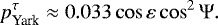 (A.2)
(A.2)
For the thermal parameters θ that are far away from unity, pYark can be substantially less. Even so, from Table 1 in Golubov & Krugly (2012) we can see that for the main-belt asteroids covered with regolith we have θ ~ 1, thus  is close to or somewhat less than Eq. (A.2).
Substituting Eq. (A.2) into Eq. (A.1), performing the inte- gration, and assuming ε = 0, we get
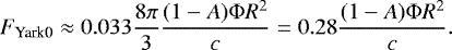 (A.3)
(A.3)
If ε is large or θ is far away from unity, the actual value of the Yarkovsky effect can be anywhere in the range between − FYark0 and FYark0.
References
- Galád, A. 2012, A&A, 548, A25 [NASA ADS] [CrossRef] [EDP Sciences] [Google Scholar]
- Golubov, O., & Krugly, Y. N. 2012, ApJ, 752, L11 [NASA ADS] [CrossRef] [Google Scholar]
- Golubov, O., & Scheeres, D. J. 2019, AJ, 157, 105 [NASA ADS] [CrossRef] [Google Scholar]
- Golubov, O., Kravets, Y., Krugly, Y. N., & Scheeres, D. J. 2016, MNRAS, 458, 3977 [NASA ADS] [CrossRef] [Google Scholar]
- Harris, A. W., & Harris, A. W. 1997, Icarus, 126, 450 [Google Scholar]
- Ivezić, Ž., Tabachnik, S., Rafikov, R., et al. 2001, AJ, 122, 2749 [Google Scholar]
- Jacobson, S. A., & Scheeres, D. J. 2011, Icarus, 214, 161 [CrossRef] [Google Scholar]
- Johnston, W. R., Asteroid pairs and clusters, last updated 11 January 2020, http://www.johnstonsarchive.net/astro/asteroidpairs.html [Google Scholar]
- Michel, P., Richardson, D. C., Durda, D. D., Jutzi, M., & Asphaug, E. 2015, Asteroids IV, Collisional Formation and Modeling of Asteroid Families (Tucson: University of Arizona Press), 341 [Google Scholar]
- Nesvorný, D., & Vokrouhlický, D. 2006, AJ, 132, 1950 [Google Scholar]
- Pravec, P., & Vokrouhlický, D. 2009, Icarus, 204, 580 [NASA ADS] [CrossRef] [Google Scholar]
- Pravec, P., Fatka, P., Vokrouhlický, D., et al. 2018, Icarus, 304, 110 [Google Scholar]
- Pravec, P., Fatka, P., Vokrouhlický, D., et al. 2019, Icarus, 333, 429 [NASA ADS] [CrossRef] [Google Scholar]
- Rein, H., & Liu, S.-F. 2012, A&A, 537, A10 [Google Scholar]
- Rein, H., & Spiegel, D. S. 2015, MNRAS, 446, 1424 [Google Scholar]
- Rein, H., & Tamayo, D. 2015, MNRAS, 452, 376 [Google Scholar]
- Rein, H., Hernandez, D. M., Tamayo, D., et al. 2019, MNRAS, 485, 5490 [Google Scholar]
- Rosaev, A., & Plávalová, E. 2017, Planet. Space Sci., 140, 21 [NASA ADS] [CrossRef] [Google Scholar]
- Sergeyev, A. V., & Carry, B. 2021, A&A, 652, A59 [NASA ADS] [CrossRef] [EDP Sciences] [Google Scholar]
- Scheeres, D. J. 2007, Icarus, 188, 430 [CrossRef] [Google Scholar]
- Slyusarev, I. G. 2020, Are Large Families in The Main Belt Homogeneous, IAU General Assembly [Google Scholar]
- Vokrouhlický, D., & Nesvorný, D. 2008, AJ, 136, 280 [Google Scholar]
- Vokrouhlický, D., Bottke, W. F., Chesley, S. R., Scheeres, D. J., & Statler, T. S. 2015, Asteroids IV (Tucson: University of Arizona Press), 509 [Google Scholar]
- Vokrouhlický, D., Josef, D., Petr, P., et al. 2017, AJ, 153, 270 [CrossRef] [Google Scholar]
- Zappalà, V. 1990. A new method to identify asteroid families and assess their reliability, Nouveaux Développements en Planétologie Dynamique, 255 [Google Scholar]
- Žižka, J., Galád, A., Vokrouhlický, D., et. al. 2016, A&A, 595, A20 [NASA ADS] [CrossRef] [EDP Sciences] [Google Scholar]
JPL Small-Body Database, https://ssd.jpl.nasa.gov/sbdb.cgi
Minor Planet Center, https://minorplanetcenter.net/iau/mpc.html
NASA astrophysics data system, https://ui.adsabs.harvard.edu/
All Tables
All Figures
|
Fig. 1 Age comparison between our pipeline and the literature. The x-axis of the plot shows the formation times of these pairs taken from the literature, and the y-axis shows the corresponding times calculated by our program. The red lines are the error bars for both cases. The black dashed line represents the case when both results are in perfect agreement. |
| In the text | |
|
Fig. 2 Estimated formation times for the discovered asteroid pair candidates. These distributions include only the clones that had close encounters within the specified vesc and RHill limits. The limits are shown in the legend of each figure. |
| In the text | |
|
Fig. 3 Distribution of estimated formation times for the discovered asteroid pair candidates. Continuation of Fig. 2. |
| In the text | |
Current usage metrics show cumulative count of Article Views (full-text article views including HTML views, PDF and ePub downloads, according to the available data) and Abstracts Views on Vision4Press platform.
Data correspond to usage on the plateform after 2015. The current usage metrics is available 48-96 hours after online publication and is updated daily on week days.
Initial download of the metrics may take a while.