| Issue |
A&A
Volume 654, October 2021
|
|
|---|---|---|
| Article Number | A130 | |
| Number of page(s) | 11 | |
| Section | Atomic, molecular, and nuclear data | |
| DOI | https://doi.org/10.1051/0004-6361/202140912 | |
| Published online | 21 October 2021 | |
GSP-spec line list for the parametrisation of Gaia-RVS stellar spectra★
Université Côte d’Azur, Observatoire de la Côte d’Azur, CNRS, Laboratoire Lagrange, Bd de l’Observatoire, CS 34229,
06304
Nice Cedex 4, France
e-mail: This email address is being protected from spambots. You need JavaScript enabled to view it.
Received:
29
March
2021
Accepted:
29
June
2021
Abstract
Context. The Gaia mission is a magnitude-limited whole-sky survey that collects an impressive quantity of astrometric, spectro-photometric and spectroscopic data. Among all the on-board instruments, the Radial Velocity Spectrometer (RVS) produces millions of spectra up to a magnitude of GRVS ~ 16. For the brightest RVS targets, stellar atmospheric parameters and individual chemical abundances are automatically estimated by the Generalized Stellar Parametriser – spectroscopy group (GSP-Spec). These data will be published with the third Gaia Data Release.
Aims. Some major ingredients of the determination of these stellar parameters include the atomic and molecular line lists that are adopted to compute reference synthetic spectra, on which the parametrisation methods rely. We aim to build such a specific line list optimised for the analysis of RVS late-type star spectra.
Methods. Starting from the Gaia-ESO line lists, we first compared the observed and synthetic spectra of six well-known reference late-type stars in the wavelength range covered by the RVS instrument. We then improved the quality of the atomic data for the transitions presenting the largest mismatches.
Results. The new line list is found to produce very high-quality synthetic spectra for the tested reference stars and has thus been adopted within GSP-Spec. We note, however, that a couple of atomic line profiles, in particular the calcium infrared triplet lines, still show some deviations compared to the reference spectra, probably because of the adopted line-transfer assumptions (local thermodynamical equilibrium, hydrostatic, and no chromosphere). Future works should focus on such lines and should extend the present work towards OBA and M-type stellar spectra.
Key words: stars: abundances / atomic data / line: identification / surveys / stars: fundamental parameters
Full Table 4 is only available at the CDS via anonymous ftp to cdsarc.u-strasbg.fr (130.79.128.5) or via http://cdsarc.u-strasbg.fr/viz-bin/cat/J/A+A/654/A130
© G. Contursi et al. 2021
 Open Access article, published by EDP Sciences, under the terms of the Creative Commons Attribution License (https://creativecommons.org/licenses/by/4.0), which permits unrestricted use, distribution, and reproduction in any medium, provided the original work is properly cited.
1 Introduction
Launched in December 2013, the ESA Gaia mission is continuously surveying the sky to collect astrometric, spectro-photometric and spectroscopic data with an unprecedented precision for stars brighter than a given magnitude (down to G ~ 20.7 and ~16 for astrometry and spectroscopy, respectively). The data are then analysed by the Data Processing and Analysis Consortium (DPAC hereafter), which publishes successive versions of the Gaia catalogue (the last release being the early Data Release 3 catalogue; eDR3, Gaia Collaboration 2021). This eDR3 contains positions, parallaxes, proper motions for about 1.5 billion stars, their magnitude in the G band for around 1.8 billion stars, and radial velocities for 7.2 million stars. The complete DR3 will be published in 2022. In particular, the spectroscopic part will contain a larger catalogue of radial velocities. Stellar atmospheric parameters, chemical abundances of several chemical species, and an analysis of a diffuse interstellar band (DIB) will be also published, thanks to the parametrisation of the Radial Velocity Spectrometer data (RVS hereafter). This RVS instrument is described in detail in Cropper et al. (2018). The collected spectra cover about 25 nm around the calcium triplet infrared lines (~850 nm) at a resolution close to 11 500. These spectra are produced within the DPAC/Coordination Unit 6, which also derives the stellar radial velocities (Sartoretti et al. 2018). Then, the spectra of late-type stars are analysed by the Generalized Stellar Parametriser – spectroscopy (GSP-Spec) group (see Recio-Blanco et al. 2016, and in prep.) within the DPAC Coordination Unit 8 in order to estimate the stellar effective temperature Teff, the surface gravity log(g), the global metallicity [M/H], and the abundance of α-elements versus iron [α/Fe]. In addition, individual abundances of several chemical species are also derived. These stellar parameters and chemical abundances are automatically estimated thanks to different algorithms as the MATISSE and GAUGUIN methods (Recio-Blanco et al. 2006, 2016). Finally, an estimate of the Gaia DIB equivalent width is also performed within GSP-spec, following a specific methodology presented in Zhao et al. (2021). These parametrisation tools rely on grids of synthetic spectra that are used to train the algorithms and/or for references. Therefore, the accuracy of the derived stellar parameters depends on the quality of these reference spectra. A special effort was thus made within GSP-Spec to compute late-type star synthetic spectra as realistic as possible. In particular, producing high-quality synthetic spectra requires a collection of complete and high-quality atomic and molecular line data such as, for instance, line positions, oscillator strengths, excitation energies, and broadening parameters.
Important databases such as the Vienna Atomic Line Database (VALD hereafter, Piskunov et al. 1995, Ryabchikova et al. 2015)or the National Institute of Standards and Technology Atomic Spectra Database (NIST, hereafter) provide a huge amount of line data to synthetise stellar spectra. However, among the millions of lines that should be considered, only a small portion have precisely determined parameters. For instance, several lines observed in the solar spectrum still remain unidentified and/or are poorly synthetised. Over the years, many efforts have been made to improve the quality of such line lists by reducing the uncertainty of the transition probability (e.g. Fuhr & Wiese 2006), or the broadening parameters (e.g. Barklem et al. 2000). In this context and in order to improve the match between observed and synthetic spectra, several groups have already assembled high-quality line data to build specific line lists devoted to late-type star studies. In particular, in the wavelength range of the Ca II triplet covered by the RVS instrument, an impressive work has already been completed within the context of the Gaia ESO Survey (GES, Heiter et al. 2021) to build complete and high-quality atomic and molecular line lists. Nevertheless, the high quality and the huge quantity of RVS spectra require a specific study to check and improve (if necessary) the quality of the available line lists to infer good stellar parameters and/or chemical abundances.
The goal of the present article is to (i) quantify the quality of the available line data for modelling late-type star spectra in the RVS spectral domain, and then (ii) present an improved version of it. We first describe the adopted methodology to compare observed and simulated spectra for well-defined reference stars in Sect. 2. In Sect. 3, we quantify the quality of the GES line list and discuss the spectral transitions that should be improved. In Sect. 4, we outline how we improved the quality of the reference star synthetic spectra leading to the line list that has been adopted within GSP-Spec for the stellar parametrisation. Finally, we conclude our work in Sect. 5.
2 Selection of the reference stars: observed and computed spectra
In order to quantify the quality of a line list for the analysis of the Gaia-RVS spectra, we compare the spectra of six well-known reference stars against synthetic models both at high (R ~ 100 000) and RVS spectral resolution (R ~ 11 500). The details of the observed and synthetic spectra are explained in the following sub-sections.
2.1 Reference stars and adopted atmospheric data
Most of the RVS observed stars with accurate radial velocity estimates are of FGK spectral types. We therefore selected reference stars belonging to these types in order to check the line list quality. These references must have very well-known atmospheric parameters and individual chemical abundances together with available high-resolution (R ≫ 100 000) and high signal-to-noise ratio (S∕N ≫ 100) observed spectra covering the RVS spectral domain. We first looked for such stars in the Gaia benchmarks sample of Jofré et al. (2018) and finally selected six reference stars: μ Leo and Arcturus (two cool giant stars), 61 Cyg A, ϵ Eri, the Sun (three cool dwarfs), and Procyon (hot dwarf) since they fulfil the above criteria. Their parameters are summarised hereafter.
For the Sun, we chose the observed spectrum of Wallace et al. (2011). This spectrum was collected at the McMath-Pierce telescope with the Fourier Tranfrom Spectrometer (see Brault & Mueller 1975; Brault 1978). It was collected over the integrated solar disc with a S/N exceeding several hundreds over the whole optical domain (from 295.8 to 925.0 nm). Its spectral resolution is about 676 000 in our wavelength range.
The observed spectrum from Arcturus was taken from Hinkle et al. (2000). This spectrum covers a wide wavelength range from 372.7 to 930.0 nm with a resolution of 150 000 and a S/N around 1000. It was collected with the Coude Feed telescope on Kitt Peak using the spectrograph in the Echelle mode.
Procyon, 61 Cyg A, ϵ Eri, and μ Leo spectra were taken from the PEPSI1 database. PEPSI (Strassmeier et al. 2015, 2018) is a high-resolution (up to R ~ 270 000) echelle spectrograph for the 2 × 8.4 m Large Binoculary Telescope. It covers the optical/red domain from 383.0 to 907.0 nm and the collected spectra have typical S/Ns of several hundreds.
These selected reference stars have well-known atmospheric parameters (Teff, log(g), [Fe/H], [α/Fe]) and good data for their chemical individual abundances, microturlulent (Vmicro), macroturbulent (Vmacro), and rotational (Vsin i) velocities. The adopted values of these parameters together with their associated reference are reported in Table 1. They have been collected as follows:
The atmospheric parameters were adopted from Jofré et al. (2018). We remind the reader that in a series of articles these authors (including several groups and different technics) determined the atmopsheric parameters and individual abundances of the Gaia benchmark stars for ten chemical species from high-resolution and S/N spectra. The chemical analysis was performed by adopting independent methods and the effective temperature and surface gravity from Heiter et al. (2015) and metallicity from Jofré et al. (2014).
The broadening parameters (Vmicro, Vmacro and Vsin i) were taken from different literature sources as indicated in the notes of Table 1. For the two selected cool giants (Arcturus and μ Leo), we adopted the parameters of Hekker & Meléndez (2007). We considered those of Valenti & Fischer (2005) and Bruntt et al. (2010) for the Sun and Procyon, respectively. Finally, for 61 Cyg A and ϵ Eri, we adopted the Vsin i estimated by Benz & Mayor (1984) and Valenti & Fischer (2005), respectively; the Vmicro of Jofré et al. (2015); and the estimated Vmacro from Eq. (1) of Valenti & Fischer (2005) using our adopted Teff.
To compute accurate synthetic spectra, we also need good individual chemical abundances and, in particular those of α-elements and iron-peak elements, which are the main contributors to the spectral lines in our wavelength range. Most chemical abundances (except a few exceptions for some stars, see below) are from Jofré et al. (2018), taking into account that their solar iron abundance is equal to −0.03 dex. We defined the [α/Fe] ratio as the mean of the Mg, Si, Ca and, Ti abundances given in this compilation. We also adopted their [Fe/H] values to derive the [X/Fe] abundances since [X/H] is provided. Among the data given in Table 1, we explicitly report the [Ca/Fe] abundances used in the spectra calculation because of the presence of the important Ca II IR triplet lines found in the RVS domain. If not available in the above-cited article, we considered individual abundances scaled to the adopted [Fe/H] and [α/Fe] values.
Ideally, we also need individual abundances of carbon and nitrogen since CN is the most representative molecule in the RVS domain for the parameters of our reference stars (see Fig. 3 of de Laverny et al. 2012). Similarly, oxygen and titanium abundances are required since we notice a small contribution of TiO, especially for cool dwarf stars. Finally, FeH molecular lines may also marginally contribute to cool-star spectra. We remind the reader that Ti and Fe abundances are reported by Jofré et al. (2018).
For Arcturus, we adopted C, N, and O abundances from Ramírez & Allende Prieto (2011). These abundances were derived using atmospheric parameters that are in complete agreement with those adopted in the present work. We note that our adopted C abundance for Arcturus was derived from high-excitation C I lines and differs by around 0.4 dex from other estimations based on molecular lines (Smith et al. 2013). However, we did verify that our adopted carbon abundance leads to a better fit of Arcturus in the RVS spectral range.
For μ Leo, we adopted the C, N, and O abundances from Gratton & Sneden (1990). The atmospheric parameters adopted by these authors are again completely consistent with those of Table 1 (Teff differs by only 76 K and [Fe/H] by 0.09 dex), and these abundances can therefore be safely adopted. We note that the C abundance of these stars was estimated from molecular features.
For the three reference dwarf stars, 61 Cyg A, ϵ Eri, and Procyon, we adopted carbon and oxygen abundances from Luck (2017), although their adopted atmospheric parameters slightly differ between this study and the present work. Indeed, the effective temperatures reported by Luck (2017) are 107, 47, and 100 K higher, respectively, whereas differences in surface gravity are always lower than 0.05 dex and are thus completely compatible with ours. As discussed below in Sects. 3.2 and 3.3, we point out that for 61 Cyg A and ϵ Eri a slightly lower carbon abundance (by about −0.2 dex) leads to a better agreement between the observed and simulated spectra. Such a proposed lower carbon abundance could result from the different adopted Teff in Luck (2017) and in the present work. Since no nitrogen abundances were found for these stars, we assumed that [N/H] is scaled to [M/H].
Finally, when computing the synthetic spectra, we adopted the solar isotopic 12C/13C ratio for thedwarfs, whereas we used the ratio derived by Smith et al. (2013) for the two cool giant reference stars.
Atmospheric parameters and chemical abundances for our reference stars.
2.2 Computation of the reference stars synthetic spectra
In order to build the line list adopted for the spectral analysis conducted within GSP-Spec, we adopted in the present work exactly the same tools for computing the synthetic spectra. For that purpose, we used version 19.1.2 of the TURBOSPECTRUM2 code (Plez 2012) that computes the continuous opacity and solves the radiative transfer equation in the lines for a given model atmosphere,an assumed chemical composition and lists of atomic and molecular transitions. Line transitions are supposed to be formed under local thermodynamic equilibrium (LTE) and hydrostatic equilibrium is also assumed in the stellar atmosphere.
We adopted 1D MARCS (Gustafsson et al. 2008) model atmospheres3. These models are fully compatible with TURBOSPECTRUM and are computed with two types of geometry: plane-parallel or spherical, depending on the stellar surface gravity. Following Heiter & Eriksson (2006), we chose spherical models for log(g) ≤ 3.5 (giant stars, g in cm s−2) and plane-parallel geometry when log(g) > 3.5 (dwarf stars). For each reference star of Sect. 2.1, we used the tool available on the MARCS website in order to interpolate a specific model atmopshere at the atmospheric parameters of Table 1.
On the other hand, the chemical abundances of each star reported in Table 1 were considered in TURBOSPECTRUM. For the Sun and as adopted in the MARCS models, we used Grevesse et al. (2007) chemical abundances and isotopic compositions. The code also takes into account the microturbulence parameter (Vmicro), whereas macroturbulent (Vmacro) and rotational velocities (Vsin i) were considered afterwards by convolving the computed spectra with the required broadening profiles. We note that we used a radial-tangent profile for the macroturbulence. References for these velocity parameters are also given in Table 1.
The last (and for our purpose most important) ingredients required to compute synthetic spectra are the atomic and molecular line lists. As a first try, we started this study by adopting the line lists provided by the line list group of the Gaia ESO Survey Heiter et al. (2021). For the atomic lines, they started with line data extracted from the VALD database4 and then optimised the selected data for the analysis of FGK-type spectra by generally favouring experimental atomic data. This line list takes into account hyperfine structures (hfs), isotopic splitting, and up-to-date broadening due to collisions with neutral hydrogen atoms. For the molecular transitions, we considered the line lists from the following species (mostly from GES): 12CH and 13CH (Masseron et al. 2014), 12C12C (Brooke et al. 2013), 12C14N (Brooke et al. 2014), 12C15N and 13C14N (Sneden et al. 2014), CaH and ZrO (including the isotopologues 90−92,94,96Zr, B. Plez, priv. comm.), OH (T. Masseron, priv. comm.), SiH (Kurucz 2010), and FeH (Dulick et al. 2003). We point out that, contrarily to GES, we adopted the most recent, complete, and accurate available line lists for VO (McKemmish et al. 2016) and TiO (McKemmish et al. 2019, including its isotopologues 46−50TiO). For this TiO line list, these authors indeed pointed out its better quality with respect to previous ones for simulating cool star spectra. The better quality of these TiO line data was recently confirmed by Pavlenko et al. (2020) for cool stars in which these lines become dominant. Of particular interest for RVS spectra, they found substantial improvement in the 840–850 nm region. Good improvements are also found in 850–880 nm, but they noticed that new laboratory measurements with smaller uncertainties in this region of the E-X 0-0 band could help to further improve the present line list quality. Since no lines from 12C13C, 13C13C, NH, and 24−25−26MgH were found in the RVS domain, these species were thus discarded. In total, our line list is composed of millions of molecular lines and a couple of thousand atomic lines. We point out that most of the adopted data are mainly composed by empirically or theoretical (and therefore not measured) atomic/molecular data and the quality of some of them could therefore still be checked. We hereafter refer to this line list as the ‘GES’ one since most data come from Heiter et al. (2021).
Finally, we computed the reference stars’ synthetic spectra with an initial wavelength step of 0.001 nm between 846.0 nm and 870.0 nm in order to cover the RVS spectral range. This led to synthetic spectra with 24 000 wavelength points (wlp, hereafter). We then convolved them to produce high-resolution (R = 100 000) and RVS-like resolution (R = 11 500) spectra, assuming a Gaussian profile to mimic the instrumental effect. The RVS-like spectra have then been re-binned with 800 wlp to satisfy the Nyquist-Shannon sampling criterion.
Quality-fit parameters (QFP) computed from the comparison between the synthetic and observed spectra at R = 11 500 (800 wlp) for the GES line list, the complete GSP-Spec line list (GL), or rejecting the core of the calcium triplet lines (GLnoCaT).
3 Comparison between the observed and computed spectra for the GES line list
We now compare the observed and simulated spectra at high and low spectral resolutions (R = 100 000 and 11 500) over the spectral domain [846.0–870.0 nm] with 24 000 and 800 wlp, respectively.Choosing these two resolutions allowed us to (i) quantify the consistency between the computed and observed spectra for RVS-likedata, (ii) more easily detect the problematic lines since, thanks to the high resolution, blends are more easily identified, and (iii) improve the line list quality by calibrating identified problematic lines if necessary (see next section).
In order to quantify the possible mismatches between observed and computed spectra, they were compared in the vacuum with Gaia spectra for consistency. We point out that the line list presented above contains air wavelengths and, thus, the spectra are computed in the air. The air-to-vacuum conversion of the fluxes was then done afterwards thanks to the relation given in Birch & Downs (1994). To quantify the differences, we introduced the following quality fit parameters (QFP):
First, the flux difference is quantified by χ2 =  (M[i]−O[i])2, with M and O being the synthetic and observed spectra, respectively. Nwlp, the number of wlp, is equal to 24 000 or 800, depending on the spectral resolution.
Then N1, N3, N5 are the number of wlp for which a difference between the synthetic and observed normalised fluxes are between 1 and 3%, between 3 and 5%, and higher than 5%, respectively.
Tables 2 and 3 present these QFP for the six selected reference stars computed at R = 11 500 and 100 000, respectively. In both tables and for each star, the first column refers to the QFP for the synthetic spectra computed with the GES line list presented above in Sect. 2.2. In order to more easily identify possible mismatches between observed and computed spectra, we calculated these QFP with and without considering the calcium triplet lines (GESnoCaT in the second columns of both tables) since accurately simulating their core could be problematic because of NLTE and/or chromospheric effects. For this GESnoCaT case, we excluded a window of ~2 nm width centred at the core of the three Ca II lines. The discarded wavelength ranges are (in vacuum and nm): [849.43–851.03], [853.73–855.73], and [865.74–867.74].
In the present section, we mostly focus on the results presented in Table 2 for the Gaia-RVS spectral resolution but the same tendency is also seen at higher resolution (Table 3). First, we discuss the impact of the metallicity on the fit quality for the two reference cool giant stars in Sect. 3.1 Then, we inspect the importance of the temperature on the QFP by examining the dwarf spectra in Sect. 3.2. Finally, we examine the effect of the surface gravity on the fit quality by comparing spectra of dwarfs and giants with close Teff (Sect. 3.3).
3.1 Cool giant stars
First of all, we notice that among the two cool giants, Arcturus exhibits the best fit both at high and low spectral resolution. For example, the χ2 and the number of wlp with a difference between 3 and 5% (N3) vary by more than a factor of two at high resolution between these two giant stars. The reason is that, although their rather similar Teff and log(g), Arcturus’ spectrum exhibits far fewer lines than μ Leo because it is more metal poor (μ Leo being ~0.75 dex more metal rich, see Table 1). It is therefore much easier to produce a more realistic spectrum and, hence, better QFP for Arcturus.
Moreover, for both stars (but this is also true for any other reference star), the large difference between N1 and N3 (or N5) is mostly dominated by molecular transitions that are predominantly fainter. We point out that in these cool giant stars, the CN molecule is the dominant species (TiO lines beginning to be visible only for Teff ≲ 4100 K). We also checked that, for any cool stars, atomic lines mostly contribute to the major mismatches (N3 and N5). Therefore, the huge number of molecular transitions that appear in the metal-rich spectrum of μ Leo explains its much larger N1 with respect to other reference stars at low resolution.
Furthermore, by looking for each star at the column GESnoCaT of Table 2, it is remarkable that the calcium triplet lines considerably impact the fit quality. For instance, if we do not consider this triplet for Arcturus, the largest mismatches in flux (N5 and N3) completely disappear at the RVS resolution, although smaller differences (N1) are still present but they are less numerous. However, there are still some large discrepancies at higher resolution for Arcturus, mainly caused by atomic lines that require some improvements (see Sect. 4). Similar conclusions are obtained for the μ Leo spectrum when removing these calcium lines.
3.2 Dwarf stars
First, when comparing the three coolest dwarf stars (61 Cyg A, ϵ Eri, and the Sun), we notice that there is a very good agreement between observed and synthetic spectra at the RVS resolution both in terms of N5 and N3, particularly if one disregards the calcium triplet lines. However, smaller flux differences (N1) are still numerous and are again dominated mostly by molecular lines.
Then, since the surface gravities are similar and the metallicities almost do not differ among these dwarfs, the main parameter that affects their fit quality is the effective temperature that varies by about 1400 K. In particular, Teff plays a crucial role since it governs the presence or absence of both atomic and (most importantly for N1) molecular lines. Regarding these molecular transitions, Fig. 1 (top panel) shows the difference between a spectrum calculated with only CN and TiO lines (including all their respective isotopes) at the low effective temperatures for which molecular lines are important in the stellar spectra (although still present but very weak at ~5750 K). We remind the reader that these two molecules are the most important ones for the selected reference stars and spectral domain. These dwarf spectra differences were calculated assuming [Fe/H] = [α/Fe] = 0.0 dex, log(g) = 4.5, and Vmicro = 1.0 km s−1 at the RVS resolution. No broadening due to Vmacro and Vsin i were considered. When the difference between the CN and TiO contributions to the spectra is positive (negative), this means that the TiO lines contribute more (less) than CN ones (green and red backgrounds, respectively). First, we point out that for Teff ≲ 4000 K and Teff ≳ 4300 K, these two molecules almost do not coexist in dwarf spectra: TiO being present/absent (and CN absent/present) for these two temperature regimes, respectively. Moreover, it is noticeable that below ~4000 K, TiO is by far the dominant absorbing species. On the contrary, for larger Teff, the contribution of CN becomes dominant and reaches a maximum around ~5000 K, corresponding to the effective temperature of ϵ Eri. This is the main reason why this star has the worst fit with respect to the two other cool dwarfs: far more molecular (CN) lines are present in its spectrum. All of this can be explained by (i) the smaller dissociation energy of TiO with respect to CN, favouring the formation of CN at effective temperature hotter than ~4300 K; and (ii) at lower temperatures, the formation of TiO is favoured since most carbon atoms are blocked onto CO molecules and, with oxygen being more abundant than carbon, almost no CN molecules can be formed. Finally, for even larger Teff (becoming closer to the solar value), the contribution of the CN molecule decreases and becomes negligible since the stellar atmopshere becomes too hot to favour molecular formation. Nevertheless, one also notices that, for ϵ Eri, a better fit of the CN lines (and an improvement of all its QFP) would be obtained by adopting a slightly lower carbon abundance (about −0.2 dex). Decreasing the nitrogen abundance does not improve the global fit as well. Such a proposed lower carbon abundance would result from the slightly hotter Teff (with respect to us) adopted in Luck (2017) when deriving their C abundance in 61 Cyg A.
However, one can also see in both tables that N5 and N3 are better for 61 Cyg A than for the hotter Sun. This is interpreted by (i) the larger metallicity of the Sun leading to the formation of more lines in its spectrum although its larger Teff, and (ii) the better fit of the calcium IR triplet lines (including the wings) in 61 Cyg A. By looking at the GESnoCaT column of Tables 2 and 3, it is noticeable that, without the calcium triplet lines, all the QFP (except N3 and N5 at high resolution) become smaller for the Sun than for 61 Cyg A. One can also see that the atomic lines in the solar spectrum are rather well synthesised (very good N5 and N3 at 11 500). This probably results from the fact that atomic line data are predominantly checked and/or optimised for this very well-studied reference star.
Finally, it is well known that the effective temperature also acts on the number of atomic lines in stellar spectra: a hot spectrum exhibits fewer atomic lines than a cooler one at constant metallicity. It is therefore logical that a good fit of hot star spectra should be easier to achieve with respect to cooler ones because of the difficulty to obtain accurate atomic and molecular line data. This is confirmed by the QFP reported in Tables 2 and 3, where it is noticeable that Procyon shows a better fit than ϵ Eri (neglecting the calcium triplet lines). If one neglects these three calcium lines, the fit of Procyon becomes as good as the one of 61 Cyg A and the Sun. It is, however, slightly worse than in the Sun since some atomic linespredominantly formed in the hottest stellar atmosphere (particularly seen at high resolution in N3 and N5) still need to be improved.
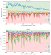 |
Fig. 1 Differences between synthetic spectra (normalised flux) computed with only CN and TiO lines for five values of the effective temperature. The spectra were computed adopting [Fe/H] = [α/Fe] = 0.0 dex with R = 11 500 and 800 wlp for typical dwarf (log(g) = 4.5, Vmicro = 1.0 km s−1) and giant stars (log(g) = 1.5, Vmicro = 2.0 km s−1), top and bottom panels, respectively. Green and red background colours refer to dominant contributions of TiO and CN, respectively. |
3.3 Comparing dwarfs and giants of similar effective temperatures
We now examine the effects of the stellar surface gravities on the fit quality by comparing the QFP for 61 Cyg A and Arcturus, which differ by about 3 dex in log(g) but have almost similar Teff and [Fe/H]. Looking at the first column for both stars in Tables 2 and 3, we first notice that the largest mismatches expressed through N3 and N5 are much larger in Arcturus than in 61 Cyg A. Comparing for these two stars the second column of these tables, we can see that these large differences are mainly caused by the rather bad fit of the calcium triplet lines. Hence, removing them for the estimation of the QFP produces at low resolution (especially for these two stars) a fit of very good quality, except for the smallest flux differences (N1). These smallest mismatches are more numerous for 61 Cyg A than for Arcturus. By comparing the top (dwarfs) and bottom (giants) panels of Fig. 1, one can see that, at the studied Teff (~4300 K), the contribution of CN is much stronger in giants than in dwarfs (TiO being almost unformed in both stars). We note that, in the bottom panel, we adopted log(g) = 1.5 and Vmacro = 2.0 km s−1 (the other parameters being similar to those adopted for dwarfs in the top panel). However, although fainter in 61 Cyg A, we checked that its CN lines are not as well fitted as in Arcturus and produce its higher N1. This could again be solved by adopting a lower carbon abundance by about ~0.2 dex in 61 Cyg A, as we already proposed for ϵ Eri. Again, this proposed smaller [C/Fe] could result from the hotter Teff adopted by Luck (2017). Slightly decreasing the carbon abundance in this star leads to a much better fit and a two-times-lower N1 (thus becoming smaller than in Arcturus). Finally, we note that, apart from the calcium triplet lines, the majority of the largest mismatches between the observed and simulated spectra (especially at high resolution) for these two cool stars are caused by atomic lines whose fit could be improved.
4 The GSP-Spec line list
Although the global agreement between the observed and simulated spectra appears already rather good, there are still some important local disagreements revealed by poorly synthesised spectral lines. Apart from the calcium triplet lines, most of the largest spectra differences (N3 and N5) for the reference stars are caused by atomic transitions. To improve this situation, we therefore decided to build a new atomic line list, startingfrom the one presented in Sect. 2.2. We remind the reader that we only focus on the atomic transitions since they play a crucial role in the atmospheric parameter and abundance derivations performed within GSP-Spec. This new line list was created by (i) identifying the atomic transitions (and associated possible blends) causing the largest mismatches between the observed and simulated high-resolution spectra, and then (ii) calibrating the atomic data of these identified lines. This new list is called the GSP-Spec line list hereafter (GL).
4.1 Astrophysical calibration of some atomic lines
We started by identifying the atomic transitions leading to the highest mismatches at both high and low resolution thanks to the N3 and N5 QFP. Among the detected lines with uncertainties in the line positions, we only had to slightly correct the wavelength of the multiplet 6 of S I. We adopted 869.5524, 869.6319, and 869.7014 nm in vacuum (869.3137, 869.3931, and 869.4626 nm in air), in perfect agreement with Wiese et al. (1969).
Then, for all the other identified lines, it appeared necessary to only correct their oscillator strength (gf) without changing any other of their line data such as their broadening parameters. These gf were first ‘astrophysically’ calibrated to improve the fit quality (visual inspection of the fit and check of the QFP) and match the solar spectrum as well as possible. We checked that this calibration also improved the Arcturus and Procyon fits, these being the best known stars among cool giants and hot dwarfs. For this calibration, we always assumed the chemical abundances reported in Table 1. Finally, as is shown Sect. 4.2, these modified oscillator strengths improve the fit quality of all of our other reference stars.
In total, we calibrated about 170 atomic oscillator strengths belonging to about ten different atomic species (whatever their isotope and ionisation state) among the ~70 chemical elements present in the line list. All these calibrated transitions are listed in Table 4. The distribution of the differences between the initial and calibrated oscillator strengths is shown in Fig. 2 (excluding the potential Fe II line discussed hereafter because of its unknown real nature). The mean change in log(gf) is 0.30 dex and 50, 80, 95% of the lines were corrected by less than 0.15, 0.50, and 1.10 dex, respectively. Moreover, no systematic changes for a given species are noticed. These corrections lead to changes of up to a few percent in the flux of some lines at the RVS resolution. Regarding the three huge calcium triplet lines that were causing the largest differences between observed and synthetic spectra, we slightly decreased their oscillator strengths by 0.024/0.037/0.027 dex, favouring the fit quality of the calcium wings since they contribute to several blends. This led to a well-improved wing fit, although it was not perfect in all the reference stars since different behaviours in the line profiles are seen among these stars. We note, however, that it was impossible to simultaneously well fit both the core and the wings of these calcium lines with the adopted physical assumptions since these cores are probably subject to NLTE and/or chromospheric effects. Perfectly fitting both the cores and the wings of these CaT lines would indeed require a more realistic treatment of the radiative transfer in these stellar atmospheres, which is beyond the scope of the present work.
Finally, we remarked a line present in the observed spectrum of Procyon and also visible although fainter in the solar spectrum (with a normalised flux of 0.95 and 0.97%, at the RVS resolution, respectively). By looking at spectra of stars hotter than Procyon, we verified that this line becomes stronger for hotter Teff, suggesting that it belongs to an ionised element and/or has a high excitation energy. This line is found in vacuum around 858.794 nm (~858.558 nm in air) and is absent from our synthetic spectra whatever the effective temperature is. This unknown line is therefore missing in the GES line list or has incorrect atomic parameters. In order to identify it, we searched the VALD and NIST databases as well as in Kurucz website5 for all lines between 858.500 and 858.600 nm (in air). First, we point out that Moore et al. (1966) identified this line as S I, but since no such sulfur line was reported by line databases, we discarded this proposition. Then, the most likely candidates found were the Fe II (858.544 nm in air; 858.779 nm in vacuum) and Sr III (858.552 in air; 858.788 nm in vacuum) lines. The excitation energy of the latter (33 ev) seems to be too high to be observed in stars of temperature smaller than 8000 K. The other candidate lines being too distant in wavelength and/or too weak, we therefore considered this line as corresponding to the Fe II transition that was already present in the original GES list but with a far too weak oscillator strength. In order to well fit our hot reference star spectra, we had to calibrate its wavelength and gf, which was increased by 8.786 dex. We also note that this line seems to be blended by another unidentified line (around 858.850 nm in vacuum) that appears much weaker in Procyon and solar spectra. Nevertheless, this tentative Fe II line was adopted in our GSP-Spec line list and well improves the fit quality of the hot star spectra. Its Fe II-nature should be confirmed later by comparison with the abundances derived from other independent iron lines when analysing hot star spectra within GSP-Spec.
Calibrated atomic lines.
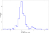 |
Fig. 2 Distribution of the differences between the initial and adopted oscillator strengths for the astrophysically calibrated lines of the GSP-Spec line list. |
4.2 Quality of the GSP-Spec line list
To quantify the quality of the new fits between the observed and simulated spectra adopting the improved GSP-Spec line list, Table 5 presents the new computed QFP at the RVS resolution. It is built as Table 2, to which it should be compared. The first column for each reference star (‘GL’) refers to the QFP corresponding to the final adopted line list (the spectra being computed exactly as those described in Sect. 2.2). The second column of each reference star (GLnoCaT) shows the QFP by disregarding ~2 nm at the core of the three Ca II lines as previously done.
First, it can be clearly seen that a global improvement of the fit quality of any reference star is obtained when adopting the GSP-Spec line list: the χ2 are smaller and most of the mismatches previously reported have indeed disappeared. For instance, if one disregards the CaT lines, N5 and N3 become always null, except for a few wlp in μ Leo caused by molecular lines and only one wlp in ϵ Eri (a Si I line not well fitted only in this star, suggesting a possible different Si abundance than the one adopted). A gain of about a factor of two in N3 is obtained for ϵ Eri, the Sun, and Procyon, considering the complete spectral domain. The gain in N1 is also important, particularly for the Sun.
The improved fit quality is also illustrated in Figs. 3–8, which show the observed (in blue) and synthetic (in orange) spectra for the six reference stars at the RVS spectral resolution (these star global fits are ordered as in Table 1). One can again see an excellent global match between both spectra, confirming the good QFP reported in column GL of Table 5. Visually, the Sun and 61 Cyg A exhibits the best fits, whereas μ Leo shows the largest mismatches. We can also remark that the largest mismatches (shown by green and red vertical dashed lines corresponding to N3 and N5, respectively) originate from the calcium triplet lines. Both the cores (for all the stars excepted 61 Cyg A) and wings (especially for Procyon) are responsible for the main discrepancies. However, we highlight the good fit of the wings of triplet calcium lines for the Sun.
In summary, if one disregards the calcium triplet lines and some faint molecular lines causing most of the small differences in the coolest stars, the derived GSP-Spec line list strongly improves the fit quality for the studied reference stars. This new line list can therefore be safely adopted for the analysis of Gaia/RVS spectroscopic data.
Quality-fit parameters computed from the comparison between the synthetic and observed spectra at R = 11 500 (800 wlp) for the complete GSP-Spec line list (GL) and rejecting the core of the Calcium triplet lines (GLnoCaT).
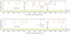 |
Fig. 3 Observed (blue) and synthetic (orange) spectra for Arcturus. Vertical green and orange dashed lines identify spectral lines differing by between 3 and 5% and by more than 5% in relative flux, respectively. These spectra were computed adopting the final GSP-Spec line list and are shown at the RVS spectral resolution with 800 wlp. We note that the wavelengths are shown in vacuum. Some line identifications are shown for non-blended absorption lines with a normalised flux below 0.93. The lower yellow insets show the difference between the observed and synthetic fluxes. |
5 Conclusion
The automatic analysis of Gaia-RVS spectra performed by the DPAC/GSP-Spec group in order to estimate the atmospheric parameters and individual chemical abundances of late-type stars relies on synthetic spectra grids. To compute high-quality spectra for such cool stars, good quality line data are required. In this article, we thus present the line list that was adopted within GSP-Spec.
In order to quantify the line list quality, we first selected six very well-parametrised reference giant and dwarf stars with effective temperatures ranging from ~4200 to ~6500 K, that is, representingthe typical Teff of the stars presently analysed within GSP-Spec. Observed high-resolution and high-S/N spectra covering the RVS spectral domain were retrieved for these reference stars. Then, high-resolution synthetic spectra were computed for these reference stars thanks to the TURBOSPECTRUM v19.1.2 radiative transfer code and MARCS model atmosphere.
Stellar synthetic spectra were first computed by adopting the line list built by the Gaia-ESO Survey consortium. The quality of this GES line list was quantified by comparing the observed and simulated spectra at high (R = 100 000) and RVS-like spectral resolution (R = 11 500). A rather good global agreement for the six reference stars is found, although some important line mismatches are reported. For instance, relative flux differences larger than 3% are identified for 162 atomic transitions. Smaller disagreements (typically of the order of 1%) are mostly caused by molecular transitions. We find that most of the atomic line mismatches can be solved by correcting the adopted atomic line data and that the possible incompleteness of the line list has a minor impact. We therefore carefully checked the quality of these line data and, when necessary, we astrophysically calibrated several atomic oscillator strengths (a couple of line positions were also corrected) in order to fit the observed reference star spectra as well as possible. The improvement of the flux fit quality adopting this GSP-Spec line list was quantified and is found to be important. This new line list produces still not perfect synthetic spectra, however, for every type of star, since a few lines are found to be sometimes not perfectly well reproduced. In particular, the ionised calcium triplet lines exhibit mismatches in their core and/or wings, probably due to NLTE and/or chromospheric effects not considered in the adopted synthesis tools.
Finally, since the new GSP-Spec line list is found to produce better and more realistic synthetic spectra, it was adopted for the GSP-Spec analysis performed for the thirst data release of Gaia. This line list can be retrieved by contacting the authors of the present article. However, we warn that it was optimised in the MARCS models and TURBOSPECTRUM v19.1.2 contexts and should therefore be used with these same tools. Finally, we notice that no optimisation of the molecular transitions were performed, and the fit quality outside the 4000–8000 K effective temperature regimes was not checked. Future extensions of the present work should first focus on these cooler and hotter stars. More realistic physical assumptions such as NLTE and 3D hydrodynamical simulations should also be investigated. Considering the Stark line broadening may also help to better reproduce some line profiles such as the calcium triplet lines.
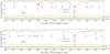 |
Fig. 7 Same as Fig. 3, but for the Sun, which has identified lines that have a depth lower than 0.97. |
Acknowledgements
The authors warmly thank Bengt Edvardsson for sharing his fruitfull experience for building line list. We are grateful to M.T. Belmonte Sainz-Ezquerra, Y. Frémat, A. Lobel, J. Pickering, and N. Ryde for discussions on some specific atomic transitions.The huge efforts performed by the GES line list group to produce their lists are also thanked. We acknowledge M. Bergemann for providing this GES line list in TURBOSPECTRUM format. We also sincerely thank the stellar atmosphere group in Uppsala for providing the MARCS model atmospheres to the community, B. Plez for having developped and maintaining the TURBOSPECTRUM package and, all the atomic/molecular line list providers. In particular, B. Plez and T. Masseron are acknowledged for having provided some molecular line lists. This work has made use of the VALD database, operated at Uppsala University, the Institute of Astronomy RAS in Moscow, and the University of Vienna. We also used the SIMBAD database, operated at CDS, Strasbourg, France. Part of the calculations have been performed with the high-performance computing facility SIGAMM, hosted by OCA. Finally, we thank the anonymous referee for their valuable comments.
References
- Barklem, P. S., Piskunov, N., & O’Mara, B. J. 2000, A&AS, 142, 467 [NASA ADS] [CrossRef] [EDP Sciences] [Google Scholar]
- Benz, W., & Mayor, M. 1984, A&A, 138, 183 [NASA ADS] [Google Scholar]
- Birch, K. P., & Downs, M. J. 1994, Metrologia, 31, 315 [NASA ADS] [CrossRef] [Google Scholar]
- Brault, J. W. 1978, in Future solar optical observations needs and constraints, ed. G. Godoli (Italy: Pubblicazioni della Universita degli Studi di Firenze), 106, 33 [NASA ADS] [Google Scholar]
- Brault, J. W.,& Mueller, E. A. 1975, Sol. Phys., 41, 43 [NASA ADS] [CrossRef] [Google Scholar]
- Brooke, J. S. A., Bernath, P. F., Schmidt, T. W., & Bacskay, G. B. 2013, J. Quant. Spectr. Rad. Transf., 124, 11 [Google Scholar]
- Brooke, J. S. A., Ram, R. S., Western, C. M., et al. 2014, ApJS, 210, 23 [NASA ADS] [CrossRef] [Google Scholar]
- Bruntt, H., Bedding, T. R., Quirion, P. O., et al. 2010, MNRAS, 405, 1907 [Google Scholar]
- Cropper, M., Katz, D., Sartoretti, P., et al. 2018, A&A, 616, A5 [NASA ADS] [CrossRef] [EDP Sciences] [Google Scholar]
- de Laverny, P., Recio-Blanco, A., Worley, C. C., & Plez, B. 2012, A&A, 544, A126 [NASA ADS] [CrossRef] [EDP Sciences] [Google Scholar]
- Dulick, M., Bauschlicher, C. W., J., Burrows, A., et al. 2003, ApJ, 594, 651 [NASA ADS] [CrossRef] [Google Scholar]
- Fuhr, J. R., & Wiese, W. L. 2006, J. Phys. Chem. Ref. Data, 35, 1669 [NASA ADS] [CrossRef] [Google Scholar]
- Gaia Collaboration (Brown, A. G. A., et al.) 2021, A&A, 649, A1 [NASA ADS] [CrossRef] [EDP Sciences] [Google Scholar]
- Gratton, R. G., & Sneden, C. 1990, A&A, 234, 366 [NASA ADS] [Google Scholar]
- Grevesse, N., Asplund, M., & Sauval, A. J. 2007, Space Sci. Rev., 130, 105 [Google Scholar]
- Gustafsson, B., Edvardsson, B., Eriksson, K., et al. 2008, A&A, 486, 951 [NASA ADS] [CrossRef] [EDP Sciences] [Google Scholar]
- Heiter, U., & Eriksson, K. 2006, A&A, 452, 1039 [NASA ADS] [CrossRef] [EDP Sciences] [Google Scholar]
- Heiter, U., Jofré, P., Gustafsson, B., et al. 2015, A&A, 582, A49 [NASA ADS] [CrossRef] [EDP Sciences] [Google Scholar]
- Heiter, U., Lind, K., Bergemann, M., et al. 2021, A&A, 645, A106 [EDP Sciences] [Google Scholar]
- Hekker, S., & Meléndez, J. 2007, A&A, 475, 1003 [NASA ADS] [CrossRef] [EDP Sciences] [Google Scholar]
- Hinkle, K., Wallace, L., Valenti, J., & Harmer, D. 2000, Visible and Near Infrared Atlas of the Arcturus Spectrum 3727-9300 A (USA: ASP) [Google Scholar]
- Jofré, P., Heiter, U., Soubiran, C., et al. 2014, A&A, 564, A133 [NASA ADS] [CrossRef] [EDP Sciences] [Google Scholar]
- Jofré, P., Heiter, U., Soubiran, C., et al. 2015, A&A, 582, A81 [Google Scholar]
- Jofré, P., Heiter, U., Tucci Maia, M., et al. 2018, Res. Notes Am. Astron. Soc., 2, 152 [Google Scholar]
- Kurucz, R. L. 2010, Astrophysics Source Code Library [record ascl:1205.004] [Google Scholar]
- Luck, R. E. 2017, AJ, 153, 21 [Google Scholar]
- Masseron, T., Plez, B., Van Eck, S., et al. 2014, A&A, 571, A47 [NASA ADS] [CrossRef] [EDP Sciences] [Google Scholar]
- McKemmish, L. K., Yurchenko, S. N., & Tennyson, J. 2016, MNRAS, 463, 771 [NASA ADS] [CrossRef] [Google Scholar]
- McKemmish, L. K., Masseron, T., Hoeijmakers, H. J., et al. 2019, MNRAS, 488, 2836 [Google Scholar]
- Moore, C. E., Minnaert, M. G. J., & Houtgast, J. 1966, The Solar Spectrum 2935 A to 8770 A (USA: NASA) [Google Scholar]
- Pavlenko, Y. V., Yurchenko, S. N., McKemmish, L. K., & Tennyson, J. 2020, A&A, 642, A77 [NASA ADS] [CrossRef] [EDP Sciences] [Google Scholar]
- Piskunov, N. E., Kupka, F., Ryabchikova, T. A., Weiss, W. W., & Jeffery, C. S. 1995, A&AS, 112, 525 [Google Scholar]
- Plez, B. 2012, Astrophysics Source Code Library [record ascl:1205.004] [Google Scholar]
- Ramírez, I., & Allende Prieto, C. 2011, ApJ, 743, 135 [Google Scholar]
- Recio-Blanco, A., Bijaoui, A., & de Laverny, P. 2006, MNRAS, 370, 141 [Google Scholar]
- Recio-Blanco, A., de Laverny, P., Allende Prieto, C., et al. 2016, A&A, 585, A93 [NASA ADS] [CrossRef] [EDP Sciences] [Google Scholar]
- Ryabchikova, T., Piskunov, N., Kurucz, R. L., et al. 2015, Phys. Scr., 90, 054005 [Google Scholar]
- Sartoretti, P., Katz, D., Cropper, M., et al. 2018, A&A, 616, A6 [NASA ADS] [CrossRef] [EDP Sciences] [Google Scholar]
- Smith, V. V., Cunha, K., Shetrone, M. D., et al. 2013, ApJ, 765, 16 [Google Scholar]
- Sneden, C., Lucatello, S., Ram, R. S., Brooke, J. S. A., & Bernath, P. 2014, ApJS, 214, 26 [Google Scholar]
- Strassmeier, K. G., Ilyin, I., Järvinen, A., et al. 2015, Astron. Nachr., 336, 324 [NASA ADS] [CrossRef] [Google Scholar]
- Strassmeier, K. G., Ilyin, I., Weber, M., et al. 2018, SPIE Conf. Ser., 10702, 1070212 [NASA ADS] [Google Scholar]
- Valenti, J. A., & Fischer, D. A. 2005, ApJS, 159, 141 [Google Scholar]
- Wallace, L., Hinkle, K. H., Livingston, W. C., & Davis, S. P. 2011, ApJS, 195, 6 [Google Scholar]
- Wiese, W. L., Smith, M. W., & Miles, B. M. 1969, Atomic Transition Probabilities, Sodium through Calcium, A critical data compilation (USA: University of Michigan), 2 [Google Scholar]
- Zhao, H., Schultheis, M., Recio-Blanco, A., et al. 2021, A&A, 645, A14 [NASA ADS] [CrossRef] [EDP Sciences] [Google Scholar]
More recent versions, as the 19.1.3 that considered Stark line broadening were not available when this work was performed.
All Tables
Quality-fit parameters (QFP) computed from the comparison between the synthetic and observed spectra at R = 11 500 (800 wlp) for the GES line list, the complete GSP-Spec line list (GL), or rejecting the core of the calcium triplet lines (GLnoCaT).
Quality-fit parameters computed from the comparison between the synthetic and observed spectra at R = 11 500 (800 wlp) for the complete GSP-Spec line list (GL) and rejecting the core of the Calcium triplet lines (GLnoCaT).
All Figures
|
Fig. 1 Differences between synthetic spectra (normalised flux) computed with only CN and TiO lines for five values of the effective temperature. The spectra were computed adopting [Fe/H] = [α/Fe] = 0.0 dex with R = 11 500 and 800 wlp for typical dwarf (log(g) = 4.5, Vmicro = 1.0 km s−1) and giant stars (log(g) = 1.5, Vmicro = 2.0 km s−1), top and bottom panels, respectively. Green and red background colours refer to dominant contributions of TiO and CN, respectively. |
| In the text | |
|
Fig. 2 Distribution of the differences between the initial and adopted oscillator strengths for the astrophysically calibrated lines of the GSP-Spec line list. |
| In the text | |
|
Fig. 3 Observed (blue) and synthetic (orange) spectra for Arcturus. Vertical green and orange dashed lines identify spectral lines differing by between 3 and 5% and by more than 5% in relative flux, respectively. These spectra were computed adopting the final GSP-Spec line list and are shown at the RVS spectral resolution with 800 wlp. We note that the wavelengths are shown in vacuum. Some line identifications are shown for non-blended absorption lines with a normalised flux below 0.93. The lower yellow insets show the difference between the observed and synthetic fluxes. |
| In the text | |
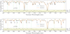 |
Fig. 4 Same as Fig. 3, but for μ Leo with an identified line with a depth lower than 0.85. |
| In the text | |
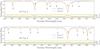 |
Fig. 5 Same as Fig. 3, but for 61 Cyg A with identified lines that have a depth lower than 0.96. |
| In the text | |
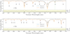 |
Fig. 6 Same as Fig. 3, but for ϵ Eri with identified lines that have a depth lower than 0.96. |
| In the text | |
|
Fig. 7 Same as Fig. 3, but for the Sun, which has identified lines that have a depth lower than 0.97. |
| In the text | |
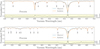 |
Fig. 8 Same as Fig. 3, but for Procyon, which has identified lines with a depth lower than 0.97. |
| In the text | |
Current usage metrics show cumulative count of Article Views (full-text article views including HTML views, PDF and ePub downloads, according to the available data) and Abstracts Views on Vision4Press platform.
Data correspond to usage on the plateform after 2015. The current usage metrics is available 48-96 hours after online publication and is updated daily on week days.
Initial download of the metrics may take a while.