| Issue |
A&A
Volume 653, September 2021
|
|
|---|---|---|
| Article Number | A38 | |
| Number of page(s) | 11 | |
| Section | The Sun and the Heliosphere | |
| DOI | https://doi.org/10.1051/0004-6361/202140498 | |
| Published online | 07 September 2021 | |
Statistical analysis of solar radio fiber bursts and relations with flares
1
Xinjiang Astronomical Observatory, Chinese Academy of Sciences, Urumqi, Xinjiang 830011, PR China
e-mail: This email address is being protected from spambots. You need JavaScript enabled to view it.
2
School of Astronomy and Space Science, University of Chinese Academy of Sciences, Beijing 100049, PR China
3
Key Laboratory of Solar Activity, National Astronomical Observatories, Chinese Academy of Sciences, Beijing 100012, PR China
Received:
4
February
2021
Accepted:
18
June
2021
Abstract
Fiber bursts are a type of fine structure that frequently occurs in solar flares. Although observations and theory of fiber bursts have been studied for decades, their microphysical process, emission mechanism, and especially the physical links with the flaring process still remain unclear. We performed a detailed statistical study of fiber bursts observed by the Chinese Solar Broadband Radio Spectrometers in Huairou with high spectral-temporal resolutions in the frequency ranges of 1.10−2.06 GHz and 2.60−3.80 GHz during 2000−2006. We identify more than 900 individual fiber bursts in 82 fiber events associated with 48 solar flares. From the soft X-ray observations of the Geostationary Operational Environmental Satellite, we found that more than 40% of fiber events occurred in the preflare and rising phases of the associated solar flares. Most fiber events are temporally associated with hard X-ray bursts observed by RHESSI or microwave bursts observed by the Nobeyama Radio Polarimaters, which implies that they are closely related to the nonthermal energetic electrons. The results indicate that most fiber bursts have a close temporal relation with energetic electrons. Most fiber bursts are strongly polarized, and their average duration, relative bandwidth, and relative frequency-drift rate are about 1.22 s, 6.31%, and −0.069 s−1. The average duration and relative bandwidth of fiber bursts increase with solar flare class. The fiber bursts associated with X-class flares have a significantly lower mean relative frequency-drift rate. The average durations in the postflare phase are clearly longer than the duration in the preflare and rising phases. The relative drift rate in the rising phase is clearly higher than that in preflare and postflare phases. The hyperbola correlation of the average duration and the relative drift rate of the fiber bursts is very interesting. These characteristics are very important for understanding the formation of solar radio fiber bursts and for revealing the nonthermal processes of the related solar flares.
Key words: Sun: corona / Sun: flares / Sun: radio radiation
© ESO 2021
1. Introduction
The radio emission of flares may provide important information for understanding the physics of flaring processes (Bastian et al. 1998). The dynamic spectrum of solar radio bursts is commonly characterized by various fine structures (FSs), such as zebra patterns, spike bursts, and even fiber bursts. These spectral FSs mainly depend on the energetic particles, on the magnetic field in the source region, and on the detailed flaring processes (Katoh et al. 2014; Tan et al. 2020). As a unique diagnostic tool for understanding the microphysical processes, solar radio FSs can provide direct information about energetic particles and the radiation source region, such as the magnetic field, the plasma parameters, particle acceleration, and propagation (Bastian et al. 1998; Aurass et al. 2005; Chernov 2006; Chen et al. 2011; Wang et al. 2017).
Radio fiber bursts belong to one of the most particular FSs embedded in the solar-type IV continuum (Young et al. 1961; Slottje 1972; Aurass et al. 1987; Chernov 2005, 2011; Huang et al. 2008, 2010). They usually appear in groups, and their prominent characteristic is the intermediate drifting rate, which is between that of type III bursts with a fast frequency-drift rate and type II bursts with slow frequency-drift rates. They are therefore also called intermediate drifting bursts (Benz & Mann 1998).
Observations of fiber bursts at meter-decimeter wavelengths have a long history that was first published by Young et al. (1961), then reported by Chernov (1976, 1990), Bernold & Treumann (1983), Aurass et al. (1987), and others. The frequencies studied in these works are in the range of below 1.0 GHz. The dynamic spectral characteristic of fiber bursts above 1 GHz were first studied by Benz & Mann (1998), and they obtained the following conclusions: (1) the relative frequency-drift rate is usually negative, with  about 0.04−0.1 s−1; (2) the duration of individual fibers is usually shorter than 1 s and the instantaneous relative bandwidth is about 2%; and (3) the absorption band (with respect to the continuum) drifts in a parallel mode and precedes the emission band.
Fiber bursts are theoretically considered as possible signatures of exciter propagation along the flare loops and mainly occur in the post-flare phase (Alissandrakis et al. 2019; Bouratzis et al. 2019). There are two major types of fiber exciter models: one is based on whistler waves (Kuijpers 1975, 1980; Mann et al. 1987), and the other is based on Alfvén waves (Bernold & Treumann 1983; Treumann et al. 1990) or fast magnetoacoustic sausage-mode waves (Kuznetsov 2006; Karlický et al. 2013). The whistler wave model involves a nonlinear interaction between whistler waves (w) and Langmuir waves (L), L + w → t, in which t is the observed electromagnetic waves. Although it can explain the frequency drift and the absorption-emission pairs of fiber bursts well, it was limited by the low efficiency of the nonlinear emission process under the typical coronal conditions (Melrose 1975). Based on these models, fiber bursts can be used to estimate the magnetic field in the source regions (Karlický et al. 2013; Wang et al. 2017; Alissandrakis et al. 2019). However, different models may derive an entirely different magnetic field strength in the source region (Benz & Mann 1998). It is necessary to determine their formation model when we apply them as a diagnostic tool of the coronal magnetic field.
A statistical study of fiber bursts may contribute to establishing general rules and setting constraints on its formation mechanisms. Elgarøy (1982) examined the characteristic parameters of fiber bursts from four frequency bands between 150 MHz and 1000 MHz, the relation between frequency-drift rate and bandwidth, the duration at a single frequency, and the scale of the source region. Benz & Mann (1998) analyzed 12 type IV continua with fiber bursts in 1−3 GHz. They made a quantitative analysis of the drift rate  and its derivative of time
  , which can be used to test the whistler wave model or the Alfvénic soliton models. Zlobec & Karlický (2014) studied 18 intervals with 700 fiber bursts at 1420 MHz and 2695 MHz during 2000−2005. They also detected more than 300 pulsations superimposed on the continuum and found that the polarizations of the fiber bursts and pulsations are similar to the continuum. They found that fiber bursts occurred in the decay or rising phase and even near the flare maximum. Using cross- and autocorrelation techniques, Bouratzis et al. (2019) analyzed 16 type IV continua with fiber bursts at a frequency of 270−450 MHz. They derived that fiber bursts had positive or negative frequency-drift rates, and the average values of the relative frequency-drift rate was around −0.027 s−1 and 0.024 s−1, respectively. They deduced a reasonable magnetic field value from the whistler wave model.
Although the observation and theoretical research of fiber bursts achieved significant progress in the past few decades, formation models are still debated. To the best of our knowledge, there is still no report about the relations of the observed parameters of fiber bursts and the flaring processes, especially at frequency above 1 GHz. This work presents a detailed investigation of fiber bursts in the frequency range of 1.10−2.06 GHz and 2.60−3.80 GHz observed by the Solar Broadband Radio Spectrometers (SBRS/Huairou) of the National Astronomical Observatories of China (NAOC) from 2000 to 2006. The observation parameters of fiber bursts in 48 flare events are detected, and the evolution of the parameters over time was analyzed. The relation of observation parameters and flare processes was studied. The observations and typical flare events are introduced in Sect. 2. Detailed descriptions of statistical analysis are presented in Sect. 3. In Sect. 4, analysis and discussion of observed parameters are implemented. Our conclusions are summarized in Sect. 5.
2. Observations and typical fiber burst events
2.1. Observations
The SBRS/Huairou is located in Beijing and began to operate during solar cycles 23 and 24. It is equipped with three telescopes that work in the 1.10−2.06 GHz, 2.60−3.80 GHz, and 5.20−7.60 GHz frequency bands (Fu et al. 2004; Tan 2008; Tan et al. 2019). The cadence is 5 ms and the frequency resolution is 4 MHz at a frequency of 1.10−2.06 GHz (the cadence was 1.25 ms in 1.10−1.34 GHz from September 2004 to October 2006). The corresponding parameters are 8 ms and 10 MHz at a frequency of 2.60−3.80 GHz, and 5 ms and 20 MHz at a frequency of 5.20−7.60 GHz. One hundred and twenty channels are used as receivers, which can automatically record the left- (L) and right- (R) handed circular polarization flux components. In order to investigate the relations between flaring process and fiber bursts, we selected the observations of solar soft X-ray (SXR) flux intensity in the 0.5−4.0 Å and 1.0−8.0 Å channel with a cadence of 3 s that were obtained by the Geostationary Operational Environmental Satellite (GOES) (Thomas et al. 1985), hard X-ray (HXR) flux obtained by the Reuven Ramaty High Energy Solar Spectroscopic Imager (RHESSI) (Lin et al. 2002), and the microwave emission intensity obtained by the Nobeyama Radio Polarimeters (NoRP) (Nakajima et al. 1985; Krucker et al. 2020). The SXR flux profiles may provide the overall temporal evolution of flaring processes, while the HXR and microwave profiles may provide important information of electron accelerations and the primary energy release (Bouratzis et al. 2015).
The radio fiber bursts usually occur in groups. We defined a relatively independent group of fibers as a fiber event that consists of dozens of individual fiber bursts. If the time interval between two fiber groups was shorter than 2 min, we considered them to be in the same event. One or more fiber events can be in a solar flare event. The smooth profile is evident at the emission ridge, and the absorption ridge may be distorted by the adjacent emission ridge and superimposition of low-intensity continuum bursts. As a result, we mainly focused on the emission ridge, and the following condition must be satisfied to ensure the statistical accuracy of each fiber parameter: (1) The observed fibers appear in groups. (2) The boundary between each fiber and the background can still be distinguished after the fiber is magnified to the pixel level. (3) Each fiber is continuous and complete. Although there are some concentrated fiber bursts near 1.10 GHz, we still measured the parameters of 937 relatively full individual fibers in 82 fiber events of 48 flares from May 2002 to September 2004 at a frequency of 1.10−2.06 GHz, from September 2004 to October 2006 at a frequency of 1.10−1.34 GHz, and from 2000 to 2006 at a frequency of 2.60−3.80 GHz. In Tables A.1 and A.2, we present the time intervals of fiber events at frequencies of 1.10−2.06 GHz and 2.60−3.80 GHz, respectively. Information about the related solar flares is also listed. From the RHESSI flare list and the microwave observations (at frequencies of 9.4, 17, or 35 GHz) of NoRP, we determined whether the fiber bursts were related to the nonthermal energetic electrons. More details are provided in Appendix A. So far, we did not distinguish any fiber structures in the frequency range of 5.20−7.60 GHz.
The starting frequency (fb), ending frequency (fe), starting time (Tb), and ending time (Te) of each individual fiber can be directly measured from the observed spectrogram (Yan et al. 2002; Tan 2008). The bandwidth df, duration D, and center frequency fc of each individual fiber are defined as df = fb − fe, D = Te − Tb, and  . The frequency-drift rate
  and the left- (L) and right- (R) handed circular polarization components can be obtained from software on the basis of the IDL algorithm. The frequency-drift rate of each individual fiber burst is almost constant. In order to compare the fibers in different frequency ranges, we adopted the relative frequency-drift rate
  and the relative bandwidth
  (with respect to the center frequency). The polarization degree is defined as
  , in which IL = L − BL and IR = R − BR represent the emission flux intensities of right and left polarization. BR and BL are background fluxes (quiet Sun, continuum) (Aschwanden 1986). Each parameter should be measured many times (more than 5), and their averaged value was adopted.
2.2. Typical examples of solar radio fiber bursts
2.2.1. Fiber bursts observed in an X1.3 flare on 30 July 2005
An X1.3 flare was observed by GOES and SBRS/Huairou in active region NOAA 10792 on 30 July 2005. Figures 1a and b plot the flaring process with the GOES SXR light curves at 1.0−8.0 Å (red), 0.5−4.0 Å (green yellow), and RHESSI HXR light curves at different energy bands. Because of the RHESSI observational gap, the data are incomplete. Figure 1a shows that the flare started at 06:17 UT, reached its maximum at 06:35 UT, and was followed by a long decay phase. According to the GOES SXR light curve at 1.0−8.0 Å, this X1.3 flare can be plotted in three phases as preflare (before 06:17 UT), rising phase (06:17 UT−06:35 UT), and postflare (after 06:35 UT) (Tan et al. 2016a). Figure 1c presents the radio flux profile at 1.2 GHz and shows that the radio bursts started at 06:20 UT and lasted until 08:00 UT. The five dotted blue lines represent the beginning time of the fiber event. Figure 1 shows that except for the first fiber event that occurred in the rising phase, all the other four fiber events occurred in the postflare phase. Figures 1d and e show the spectrograms of fiber bursts at a frequency of 1.10−1.30 GHz from 06:28:34 to 06:28:42 UT and from 07:12:13 to 07:12:33 UT, respectively.
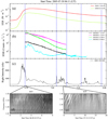 |
Fig. 1. X1.3 flare on 30 July 2005. (a): The GOES soft X-ray light curve. (b): The RHESSI hard X-ray light curve. (c): The radio flux at 1200 MHz. (d) and (e): The dynamic spectrum of the fiber bursts. |
2.2.2. Fiber bursts observed in an M4.8 flare on 12 September 2004
Figure 2 shows an M4.8 flare that took place in active region NOAA 10672 on 12 September 2004. The top panel shows the GOES SXR flux light curves at 0.5−4.0 Å and 1.0−8.0 Å. The flare started at 00:04 UT and peaked at 00:56 UT. The second panel is the HXR light curve in four energy bands during the same time interval. The radio flux profiles at 1.425 GHz obtained by SBRS/Huairou at the left-handed circular polarization (LCP) and 9.7 GHz obtained by NoRP are shown in Fig. 2c. The four dotted blue lines indicate the beginning time of the four fiber events. The two bottom panels present the dynamic spectrum observed by SBRS/Huairou in the frequency range of 1.20−1.80 GHz. We found that all fiber events occurred around the time when both HXR emissions at 25−50 keV and the microwave emissions at 9.4 GHz increased rapidly or reached a localized maximum.
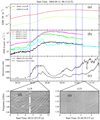 |
Fig. 2. Fiber events in an M4.9 flare on 12 September 2004. (a): The soft X-ray light curve. (b): The hard X-ray light curve. (c): The radio flux at 1425 MHz and 9.7 GHz. (d) and (e): The dynamic spectrum of two fiber events. |
2.2.3. Fiber bursts in a preflare phase on 14 January 2005
Figure 3 shows a C9.3 flare observed simultaneously by GOES, RHESSI, and SBRS/Huairou on 14 January 2005. It took place in active region NOAA 10718 located S10E02. The flare started at 03:55 UT and peaked at 04:04 UT. Figure 3a shows the SXR 0.5−4.0 Å and 1.0−8.0 Å light curve of the event from 03:35 to 04:10 UT. Figure 3b presents the HXR profiles at different energy bands. The radio flux intensity in left-handed circular polarization at 1.20 GHz from SBRS/Huairou is shown in Fig. 3c. The two dotted blue lines denote the beginning time of the two fiber burst events. As shown in Table A.1, this flare contains four fiber events. We just show the first two, which occurred in the preflare phase and very closed to the flare onset, respectively. Figures 3d and e show the dynamic spectra superimposed on the continuum in the frequency range of 1.10−1.34 GHz. These fiber bursts are strongly left-handed circular polarization. Compared to the HXR profiles, we found that about 2 or 3 min before these two preflare fiber events, small HXR peaks at 12−25 keV occurred, which might imply that the related nonthermal electrons may contribute to the fiber events.
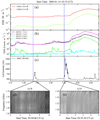 |
Fig. 3. Preflare fiber events associated with a C9.3 flare on 14 January 2005. (a): The soft X-ray light curve. (b): The hard X-ray light curve. (c): The radio flux at 1200 MHz. (d) and (e): The dynamic spectrum of fiber events. |
2.2.4. Fiber bursts at different frequency bands on 06 June 2003
Figure 4a presents the GOES SXR flux light curves at 1.0−8.0 Å and 0.5−4.0 Å of an M1.0 flare in active region NOAA 10375 on 06 June 2003. The flare started at 23:31 UT, peaked at 23:38 UT, and was followed by a long decay phase. Figure 4b shows the HXR light curves at energy bands of 3−6 keV, 6−12 keV, 12−25 keV, and 25−50 keV with black, magenta, lime, and cyan lines, respectively. Shortly after the flare onset, SBRS/Huairou detected two fiber events: the first fiber event occurred in a frequency range of 1.10−2.06 GHz from 23:33:50 UT, and the second fiber event occurred in a frequency range of 2.60−3.80 GHz from 23:35:30 UT. Figures 4c and d present the radio flux profiles and the spectrogram associated with these two fiber events. The time gap between the end of the first event and the start of the second event is only about one minute, which implies that they are related with each other. Compared to the HXR profiles (Fig. 4b), we found that these two fiber events occurred at about the time when the HXR at an energy of 12−25 keV and 25−50 keV rapidly increased. We calculated the average relative frequency-drift rates and the exciter velocities of the two fiber events, respectively. For the first fiber event, the results are about −0.079 s−1 and 7945 km s−1, and for the second fiber event in the 2.60−3.80 GHz frequency band, the results are −0.054 s−1 and 5411 km s−1. Because the exciter velocities of these two negative-drift fiber events are quite different and the fiber events in the low-frequency band are produced earlier, we suggest that the two fiber events are produced by two different acceleration processes.
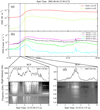 |
Fig. 4. Fiber events associated with the rising phase of an M1.0 flare on 06 June 2003. (a) The soft X-ray light curve. (b) The hard X-ray light curve. (c) The radio flux at 1160 MHz and the dynamic spectrum of the fiber event in the frequency range of 1.1−1.34 GHz. (d) The radio flux at 2840 MHz and the dynamic spectrum of the fiber event in the frequency range of 2.60−3.80 GHz. |
3. Statistics
In order to understand the physical natures of the radio fiber events and their relation with the related solar flares, we present the statistical results for the 937 individual fibers in 82 fiber events related to 48 flares. Figure 5a shows a histogram of the duration of the 915 negatively drifting fibers. It shows that the duration ranges from 0.2 s to nearly 6 s. The peak is at about 0.6 s, and most fiber bursts have a duration between 0.2 and 2.5 s. The dotted red line marks the average value, 1.22 s. As shown by the dotted yellow line in the histogram, we applied a Gaussian function and a multi-Gaussian function from the least-square method to fit the parameter to obtain the full width at half maximum (FWHM). Figure 5b shows the distribution of the relative bandwidth of individual fibers. Most fiber bursts range in relative bandwidth from 1.6% to 15%, and the average relative bandwidth is 6.31%. Figure 5c plots the distribution of the polarization degree. Negative and positive polarization denote the RCP and LCP, respectively. Figure 5c shows that most fiber bursts are strongly polarized, and the average values of RCP and LCP are −67.1% and 62.3%, respectively. Figure 5c also shows that the 915 individual fibers are roughly divided into three groups: (1) Strong RCP with a polarization degree greater than 55%, (2) strong LCP with a similarly high polarization degree, and (3) weak RCP with a polarization degree lower than 15%. Figure 5d shows the distribution of the relative frequency-drift rate  . We note that most fiber bursts have a relative frequency-drift rate in the range of −0.01 to −0.13 s−1, with peaks of about −0.05 s−1 and an average value −0.069 s−1. In addition, we also note that Fig. 5d shows a class of fast-drifting fibers that accounts for less than 8% of the fibers and has a relative frequency-drift rate
  of about −0.18 s−1, shown by the dotted black line.
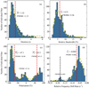 |
Fig. 5. Histograms of parameters of the 915 negative-drifting fibers. (a) Duration. (b) Relative bandwidth. (c) Polarization. (d) Relative frequency-drift rate. The dotted red line represents the average of each parameter. Panel c: mean polarization degrees of the left-handed and right-handed polarized fibers, respectively. |
The averaged parameters of 915 negative drift fibers and the corresponding histograms for different classes flares are given in Table 1 and Fig. 6, respectively. In the first column of Table 1, the number of different class flares are given. The second and third columns list the number of fiber events (Ln) and individual fibers (Fn). The fourth column D is the mean duration of individual fibers. The fifth and sixth columns are the relative bandwidth bf and relative frequency-drift rate  , respectively. The circular polarization degrees (PL and PR) are given in the last two columns. Table 1 shows that the average duration and relative bandwidth both increase with the flare level. Especially for the average duration of X-class flare fibers, it is almost twice that of C-class and M-class flare fibers. We also note that the average duration and relative bandwidth of the fiber bursts for M-class flares are almost equal to the total average duration. The relative bandwidth is given in Figs. 5a and b. Table 1 and Fig. 6d show that the average relative frequency-drift rates of fiber bursts for C-class and M-class flares are close to that given in Fig. 5d, while it is significantly lower for the X-class flares. Similar to the results in Fig. 5c, Table 1 and Fig. 6c show that most fiber bursts of the three flare classes have strong circular polarization, especially for C- and X-flares. Only a very small number of fibers have a degree of polarization lower than 50%. This indicates that the fiber bursts are closely related to the magnetic field. Table 1 also shows that fiber bursts for M-class flares have the lowest average polarization degree. By comparing Figs. 5 and 6, we can find that the parameter distribution of M-class flare fiber bursts is very similar to that in Fig. 5.
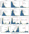 |
Fig. 6. Statistical histograms of negative-drift individual fiber parameters corresponding to C, M, and X class flares. (a) Duration. (b) Relative bandwidth. (c) Polarization. (d) Relative frequency-drift rate. The dotted red line represents the average of each parameter. Panel c: mean polarization degrees of left- and right-handed circular polarized fibers, respectively. |
Average parameters of 915 individual fibers in different fiber classes.
Table 2 presents the average parameter of the fiber bursts in different flare phases. Of the 915 individual fiber bursts, 71 (7.8%) occurred in the preflare phase, 315 (34.4%) occurred in the rising phase, and 529 (57.8%) occurred in the postflare phase. From Table 2, we can obtain several conclusions: (1) Different from the literature, which reported that most of the fiber bursts occurred in the postflare phase, almost 42% of the fiber bursts occurred in the preflare and rising phases of the flares. (2) There is no significant difference in the average duration of fiber bursts in the preflare and rising phases, while for the postflare phase, the difference is distinctly larger than that in the preflare and rising phases. (3) The relative bandwidth of fiber bursts decreases with the evolution of the flare from the preflare phase through the rising phase to the postflare phase. (4) The average relative frequency-drift rate of fiber bursts in the rising phase is significantly higher than that in the preflare and postflare phases. This indicates that the corresponding emission exciter in the rising phase should have higher velocities.
Average parameters of 915 individual fibers during different flare phases.
The solar radio spectral fine structures superimposed on the type IV continua are considered to contain important information on the particle accelerating process (Chernov 2006; Chen et al. 2011; Bouratzis et al. 2015). Fiber bursts are believed to represent the movement of some type of plasma wave excited by accelerated particles (Wang et al. 2017). In order to determine the temporal correlations between the fiber bursts with the energetic electrons, we adopted HXR observations obtained by RHESSI and microwave observations (at frequencies of 9.4, 17, or 35 GHz) obtained by NoRP. As shown in Tables A.1 and A.2, if an HXR flare or microwave bursts occurs within one minute before, after, and during the fiber event, it is marked Y, such as the examples shown in Figs. 1−4. The letter N indicates that there is no such HXR flare or microwave bursts. The minus denotes that no observation was obtained by RHESSI and NoRP during the time interval of the fiber event. The results show that most fiber events (nearly 85%) were associated with HXR or microwave bursts, which indicates that they should be related with the energetic electrons.
In addition to these statistics, we also found five groups of positive-drift fiber bursts and measured the parameters of 22 fiber bursts. These fiber bursts are indicated by a plus in Table A.1. There are two groups of positive-drift fibers in the X2.9 flare on 16 January 2005. These fibers have a comparatively high frequency-drift rate, ranging from 0.04 to 0.21 s−1, with an average of 0.12 s−1. At the same time, we also find that there are hundreds of isolated fiber bursts in the spectrum in the frequency range of 1.10−2.06 GHz from 2002 to 2006.
4. Analysis and discussion
The most special characteristic of fiber bursts is their intermediate frequency-drift rates, which are obviously higher than that of typical radio type II bursts, but much lower than the rate of type III bursts. Solar radio type II bursts with slow frequency-drift rates might be triggered by coronal mass ejections or plasma jets with velocities lower than 2000 km s−1, and solar radio type III bursts with fast frequency-drift rates might be triggered by nonthermal electron beams with a velocity of more than 0.1c (> 3 × 10⁴ km s−1) (Tan et al. 2016b). The question is what drives the formation of solar radio fiber bursts with intermediate frequency-drift rates.
4.1. Spectral characteristics of fiber bursts and their relation to solar flares
From Figs. 1−4, we can obtain several conclusions about the fiber bursts: (1) The fiber bursts can be generated in C-class, M-class, and in X-class flares. (2) The fiber bursts can occur in the preflare and rising phases as well as in the postflare phase. (3) A flare can produce fiber bursts at different frequency ranges. (4) Most fiber bursts have a high circular polarization degree. (5) There are negative-drift fibers and positive-drift fibers, and sometimes the negative- and positive-drift fibers may occur together, for example, the fiber bursts on 27 October 2003. (6) Most radio fiber bursts are associated with HXR or microwave bursts.
4.2. Deduction of the exciter speeds and magnetic fields from observations
Fiber bursts represent one type of spectral fine structures superposed on the type IV continuum (Young et al. 1961; Slottje 1972; Bouratzis et al. 2019). Several models have been proposed to explain the formation of solar radio fiber bursts: (a) The whistle-Langmuir wave-wave interaction (Kuijpers 1975, 1980), (b) Alfvén-Langmuir wave-wave interaction (Bernold & Treumann 1983), and (c) fast magnetoacoustic sausage-mode modulation (Kuznetsov 2006; Zlobec & Karlický 2014). All these models can be used to estimate the magnetic fields in the source region of fiber bursts (Benz & Mann 1998; Treumann et al. 1990; Rausche et al. 2007).
The drift rate  at frequency ν is dependent on the exciter velocity, ve, producing the fiber bursts by (Bouratzis et al. 2019)
 (1)
(1)
Here H is the scale height, depending on the temperature and gravity. θ is the propagation angle of the exciter relative to the vertical direction. If the propagation angle θ is close to zero and the ambient plasma temperature Te = 2 × 10⁶ K, H = ×105 km. According to Eq. (1), we can estimate the speed of fiber burst sources from the average frequency-drift rate listed in Tables 1 and 2. The average velocities of the emission sources in different classes of flares are about 7100 km s−1, 8100 km s−1, and 4100 km s−1 and averaged 5800 km s−1, 9700 km s−1, and 5800 km s−1 in different flaring phases. Here θ = 0°, therefore the estimated average speeds are lower limits.
At the same time, we may estimate the magnetic field in the source regions. According to the whistler wave model, the fiber bursts are caused by the parametric interaction of the low-frequency whistler waves traveling along the magnetic field and the localized Langmuir waves. Here, the frequency drift of fiber bursts is related to the group velocity vg of whistler wave, given by (Benz & Mann 1998)
 (2)
(2)
here  , ww, wce, and wpe are the whistler frequency, electron-cyclotron frequency, and plasma frequency, respectively. The whistler wave model indicates that the exciter velocity ve corresponds to the group velocity vg. By substituting vg into Eq. (1), the drifting rate can be written as
 (3)
(3)
Considering  , the magnetic field can be derived as
 (4)
(4)
Here, the unit of B is G, and the unit of ne is cm−3.
Theoretical investigation indicates that the initial value x ≈ 0.03, and decreases with propagation of whistler into weaker magnetic fields (Mann et al. 1989). Taking x = 0.01, θ = 0° and H = ×105 km, the average field strengths at 1.27 GHz (ne = 2 × 1010 cm−3) for different flare classes are about 54 G, 62 G, and 32 G, respectively. These values are very closed to the diagnosed results by Zebra patterns (Tan et al. 2012).
As for the Alfvén wave model, the fiber bursts considered as the result of plasma emission modulated by Alfvénic solitons propagating along the field lines of a coronal loop. Here, the exciter velocity ve is between 1 and 3 times the local Alfvén speed vA, defined by (Benz & Mann 1998):
 (5)
(5)
here mi is the proton mass. Assuming that the exciter velocity ve is twice vA, θ = 0° and H = ×105 km, the average field strengths of fiber sources at 1.27 GHz for the C, M, and X class are about 230 G, 263 G, and 133 G, respectively. These values are much higher than the value derived from zebra patterns (Tan et al. 2012).
Table 3 presents the exciter speeds and magnetic field strengths in the fiber sources deduced in the literature. The second column lists the frequency of fiber bursts. The third column lists the exciter speeds, which are consistent with our estimations. The magnetic field strengths estimated from the whistler waves model and magnetohydrodynamics waves model are listed in the fifth and sixth columns, respectively. Table 3 shows that the exciter speeds and magnetic field strengths increase with the frequency of the fiber bursts. As the frequencies of the fiber bursts are similar, our measurements are consistent with those of Wang et al. (2017).
Comparisons of exciter speeds and magnetic field strengths of the fiber sources.
Deducing the exciter speeds and magnetic fields in the source regions of fiber bursts is clearly dependent on the formation mechanisms. The derived exciter speeds are much higher than those of typical coronal mass ejections or any plasma jets associated with solar flares (typically, < 2000 km s−1) and clearly lower than that of the nonthermal electron beams (typically, > 0.1c, i.e., > 3 × 10⁴ km s−1). As we mentioned before, almost 85% of the fiber events are closely related with HXR or microwave bursts. The question then is what factor triggers the formation of the radio fiber bursts. However, we lack imaging observations at the corresponding frequencies, therefore it is impossible to determine which model is valid for the observed fiber bursts at present.
4.3. Estimate of the size of fiber sources
The observed bandwidth of fiber bursts is related to its source sizes. The upper limit size of individual fiber burst sources can be estimated by (Benz 1986)
 (6)
(6)
where Δf/f is the relative bandwidth. Taking H = ×105 km, the mean space scales of individual fiber bursts are about 5800 km, 6310 km, and 7200 km for C-, M-, and X-class flares, respectively.
4.4. Relation of the duration and relative frequency-drift rate
It is easy to understand that the higher the frequency-drift rate, the shorter the duration of the fiber bursts. We also hope to determine whether there are some particular correlations between these two parameters of fiber bursts.
Figure 7a shows a scatter plot of the duration of individual fiber bursts (D) with respect to the average relative frequency-drift rate ( ) in the frequency range of 1.10−2.06 GHz. We found that the relation of the duration and the frequency-drift rate of fiber bursts is not a simple linear variation, but close to a hyperbola function. Figure 7b shows the relation of the same two parameters in the frequency range of 2.60−3.80 GHz. We applied a hyperbola function from the least-squares method to fit
  and D,
 (7)
(7)
 |
Fig. 7. Duration distribution with respect to the relative frequency-drift rate of solar radio fiber bursts. The solid blue line represents the exponential fitting value. (a) In the frequency range of 1.10−2.06 GHz. (b) In the frequency range of 2.60−3.80 GHz. |
and,
 (8)
(8)
By comparison, the two sets of coefficients of Eq. (7) and Eq. (8) are very close to each other. The first coefficient of Eq. (8) is slightly larger than that of Eq. (7), possibly because the relative frequency-drift rate  distribution in the frequency range of 1.10−2.06 GHz is wider than that in the frequency range of 2.60−3.80 GHz. The large constant term of Eq. (8) may be due to the longer duration (D) of fiber bursts in the frequency range of 2.60−3.80 GHz. These two hyperbola relations also imply a lower limit of the frequency-drift rate of fiber bursts at about −0.02 s−1 in both frequency ranges of 1.10−2.06 GHz and 2.60−3.80 GHz. This lower limit tells us that all fiber bursts have a threshold of the frequency-drift rate that distinguishes it from the other types of spectral fine structures, such as type II and type IV bursts with a frequency-drift rate much slower than 0.02 s−1, and the formation mechanism of fiber bursts is also distinctly different from the others.
5. Conclusion
This work analyzed solar radio fiber bursts with a high-resolution dynamic spectrum recorded by SBRS/Huairou in the frequency ranges of 1.10−2.06 GHz and 2.60−3.80 GHz. We identified 937 individual fiber bursts in 82 fiber events associated with 48 solar flares. According to the statistical analysis of the observational parameters of fiber bursts with respect to the flare classes (C, M, and X) and flare phases (preflare, rising, and postflare), we obtained the following statistical results.
-
Different from the literature, we found that more than 40% of radio fiber events occurred in the preflare and rising phases of the associated solar flares. At the same time, most fiber events are temporally associated with hard X-ray bursts or microwave bursts, which implies that they are closely related to nonthermal energetic electrons. Even the preflare radio fiber bursts are also associated with some small HXR bursts (Fig. 3).
-
The average duration, relative bandwidth, and relative frequency-drift rate of the 915 individual fiber bursts are about 1.22 s, 6.31%, and −0.069 s−1. Most fiber bursts are strongly polarized. The average polarization degree is higher than 60%.
-
The average duration and relative bandwidth of fiber bursts increase with solar flare class. Fiber bursts associated with X-class flares have a significantly lower mean relative frequency-drift rate.
-
The average duration in the postflare phase is obviously longer than that in the first two phases. At the same time, the relative drift rate in the rising phase is obviously higher than that in preflare and postflare phases. The hyperbola correlation between the average duration and the relative drift rate of the fiber bursts is very interesting.
We also derived the magnetic field of the source region of the fiber bursts from observations near 1.27 GHz from the whistler-Langmuir wave model, which yields a magnetic field of about 55 G, 62 G, and 32 G in C-, M-, and X-class flares. These results are consistent with the diagnosed values of Wang et al. (2017) in the same frequency range, and they are also very close to the results derived from the zebra patterns observed in the same frequency range. However, these deductions clearly depend on the theoretical models. For example, the Alfvén-Langmuir wave model yields a much stronger magnetic field strength than the results derived from spectral fine structures. The largest puzzle is the velocity of the emission exciter of fiber bursts derived from the existing model, which exceeds 4000 km s−1 and no more than 104 km s−1 (see Sect. 4.2 and Table 3). This velocity is significantly faster than the localized Alfvén speed (< 2000 km s−1) but far slower than the velocity of nonthermal energetic electrons (> 3 × 10⁴ km s−1, i.e., > 0.1c). The question then is what the nature of the emission exciters is and why their velocity is so high. So far, we have no consensus. The main reason is that we have no real information about their position and the magnetic configuration of the source regions, which depends on the radio spectral-imaging observations at the corresponding frequencies. These statistical results may give us new limits for the theoretical models. In the near future, we plan to apply the new generation of solar radio spectral-imaging telescopes such as MUSER (Yan et al. 2009) to observe the radio fiber bursts and reveal their source regions and relations to the related magnetic configurations. With these observations, we may understand the formation of solar radio fiber bursts. Our next work will collect the observations from MUSER and other next-generation solar radio imaging telescopes to investigate the fiber bursts and develop a new theoretical model to explain the formation of fiber bursts.
Acknowledgments
This work is supported by 2018-XBQNXZ-A-009 and 2017-XBQNXZ-A-007, by NSFC under grant 12173076, 11673055, 11790301, 11973057 and 11773061, and by Key Laboratory of Solar Activity at National Astronomical Observatories, CAS. This work is also supported by the international collaboration of ISSI-BJ (2018YFA0404602) and the International Partnership Program of Chinese Academy of Sciences (183311KYSB20200003).
References
- Alissandrakis, C. E., Bouratzis, C., & Hillaris, A. 2019, A&A, 627, A133 [NASA ADS] [CrossRef] [EDP Sciences] [Google Scholar]
- Aschwanden, M. J. 1986, Sol. Phys., 104, 57 [NASA ADS] [CrossRef] [Google Scholar]
- Aurass, H., Chernov, G. P., Karlický, M., Kurths, J., & Mann, G. 1987, Sol. Phys., 112, 347 [NASA ADS] [CrossRef] [Google Scholar]
- Aurass, H., Rausche, G., Mann, G., & Hofmann, A. 2005, A&A, 435, 1137 [NASA ADS] [CrossRef] [EDP Sciences] [Google Scholar]
- Bastian, T. S., Benz, A. O., & Gary, D. E. 1998, ARA&A, 36, 131 [NASA ADS] [CrossRef] [Google Scholar]
- Benz, A. O. 1986, Sol. Phys., 104, 99 [NASA ADS] [CrossRef] [Google Scholar]
- Benz, A. O., & Mann, G. 1998, A&A, 333, 1034 [NASA ADS] [Google Scholar]
- Bernold, T. E. X., & Treumann, R. A. 1983, ApJ, 264, 677 [NASA ADS] [CrossRef] [Google Scholar]
- Bouratzis, C., Hillaris, A., Alissandrakis, C. E., et al. 2015, Sol. Phys., 290, 219 [NASA ADS] [CrossRef] [Google Scholar]
- Bouratzis, C., Hillaris, A., Alissandrakis, C. E., et al. 2019, A&A, 625, A58 [NASA ADS] [CrossRef] [EDP Sciences] [Google Scholar]
- Chen, B., Bastian, T. S., Gary, D. E., & Jing, J. 2011, ApJ, 736, 64 [NASA ADS] [CrossRef] [Google Scholar]
- Chernov, G. 2011, Fine Structure of Solar Radio Bursts (Berlin: Springer) [Google Scholar]
- Chernov, G. P. 1976, Sov. Astron., 20, 449 [Google Scholar]
- Chernov, G. P. 1990, Sov. Astron., 34, 66 [NASA ADS] [Google Scholar]
- Chernov, G. P. 2005, Plasma Phys. Rep., 31, 314 [NASA ADS] [CrossRef] [Google Scholar]
- Chernov, G. P. 2006, Space Sci. Rev., 127, 195 [Google Scholar]
- Elgarøy, Ø. 1982, Inst. Theor. Astrophys., 53, 30 [Google Scholar]
- Fu, Q., Ji, H., Qin, Z., et al. 2004, Sol. Phys., 222, 167 [Google Scholar]
- Huang, J., Yan, Y. H., & Liu, Y. Y. 2008, Sol. Phys., 253, 143 [NASA ADS] [CrossRef] [Google Scholar]
- Huang, J., Yan, Y., & Liu, Y. 2010, Adv. Space Res., 46, 1388 [NASA ADS] [CrossRef] [Google Scholar]
- Karlický, M., Mészárosová, H., & Jelínek, P. 2013, A&A, 550, A1 [NASA ADS] [CrossRef] [EDP Sciences] [Google Scholar]
- Katoh, Y., Iwai, K., Nishimura, Y., et al. 2014, ApJ, 787, 45 [NASA ADS] [CrossRef] [Google Scholar]
- Krucker, S., Masuda, S., & White, S. M. 2020, ApJ, 894, 158 [NASA ADS] [CrossRef] [Google Scholar]
- Kuijpers, J. 1975, Sol. Phys., 44, 173 [NASA ADS] [CrossRef] [Google Scholar]
- Kuijpers, J. 1980, Proc. IAU Symp., 86, 341 [NASA ADS] [Google Scholar]
- Kuznetsov, A. A. 2006, Sol. Phys., 237, 153 [NASA ADS] [CrossRef] [Google Scholar]
- Lin, R. P., Dennis, B. R., Hurford, G. J., et al. 2002, Sol. Phys., 210, 3 [Google Scholar]
- Mann, G., Karlicky, M., & Motschmann, U. 1987, Sol. Phys., 110, 381 [NASA ADS] [CrossRef] [Google Scholar]
- Mann, G., Baumgaertel, K., Chernov, G. P., & Karlicky, M. 1989, Sol. Phys., 120, 383 [NASA ADS] [CrossRef] [Google Scholar]
- Melrose, D. B. 1975, Aust. J. Phys., 28, 101 [CrossRef] [Google Scholar]
- Nakajima, H., Sekiguchi, H., Sawa, M., Kai, K., & Kawashima, S. 1985, PASJ, 37, 163 [NASA ADS] [Google Scholar]
- Rausche, G., Aurass, H., Mann, G., Karlický, M., & Vocks, C. 2007, Sol. Phys., 245, 327 [NASA ADS] [CrossRef] [Google Scholar]
- Slottje, C. 1972, Sol. Phys., 25, 210 [NASA ADS] [CrossRef] [Google Scholar]
- Tan, B. 2008, Sol. Phys., 253, 117 [NASA ADS] [CrossRef] [Google Scholar]
- Tan, B., Yan, Y., Tan, C., Sych, R., & Gao, G. 2012, ApJ, 744, 166 [Google Scholar]
- Tan, B., Yu, Z., Huang, J., Tan, C., & Zhang, Y. 2016a, ApJ, 833, 206 [NASA ADS] [CrossRef] [Google Scholar]
- Tan, B. -L., Karlický, M., Mészárosová, H., & Huang, G.-L. 2016b, Res. Astron. Astrophys., 16, 82 [Google Scholar]
- Tan, B.-L., Cheng, J., Tan, C.-M., & Kou, H.-X. 2019, Chin. Astron. Astrophys., 43, 59 [Google Scholar]
- Tan, B.-L., Yan, Y., Li, T., Zhang, Y., & Chen, X.-Y. 2020, Res. Astron. Astrophys., 20, 090 [Google Scholar]
- Thomas, R. J., Starr, R., & Crannell, C. J. 1985, Sol. Phys., 95, 323 [NASA ADS] [CrossRef] [Google Scholar]
- Treumann, R. A., Guedel, M., & Benz, A. O. 1990, A&A, 236, 242 [NASA ADS] [Google Scholar]
- Wang, Z., Chen, B., & Gary, D. E. 2017, ApJ, 848, 77 [NASA ADS] [CrossRef] [Google Scholar]
- Yan, Y., Tan, C., Xu, L., et al. 2002, Sci. China A: Math., 45, 89 [NASA ADS] [CrossRef] [Google Scholar]
- Yan, Y., Zhang, J., Wang, W., et al. 2009, Earth Moon Planets, 104, 97 [CrossRef] [Google Scholar]
- Young, C. W., Spencer, C. L., Moreton, G. E., & Roberts, J. A. 1961, ApJ, 133, 243 [NASA ADS] [CrossRef] [Google Scholar]
- Zlobec, P., & Karlický, M. 2014, Sol. Phys., 289, 1683 [NASA ADS] [CrossRef] [Google Scholar]
Appendix A: Time intervals of fiber burst events in different frequency ranges observed by SBRS/Huairou
Table A.1 presents 74 fiber events associated with 43 solar flares in the frequency range of 1.10−2.06 GHz. Table A.2 gives the time intervals of 8 fiber events associated with 6 solar flare recorded in the frequency range of 2.60−3.80 GHz. The first column of the tables lists the dates of the related solar flares. Columns 2–5 list the start, peak, and end times and the GOES SXR classes of the related flares. The start and end times of the fiber events are listed in Cols. 6 and 7. The last column of the tables shows whether the fiber bursts is related to the HXR bursts or microwave bursts. The HXR bursts are observed by RHESSI, and microwave bursts (at frequencies of 9.4, 17, or 35 GHz) are observed by NoRP. Here, HXR and microwave bursts are signatures of the nonthermal energetic electrons related to solar flares. Y denotes that the fiber events are temporally associated with nonthermal energetic electrons, and N indicates that there is no clearly observed evidence of nonthermal energetic electrons. The minus indicates that neither RHESSI nor NoRP have observed data during the time interval we examined. (+1) means the time is the next day, and (−1) means the time was the yesterday. (+) indicates a positive-drift fiber group.
Radio fiber burst events observed in the frequency range of 1.10−2.06 GHz and the related X-ray flares.
Radio fiber burst events observed in the frequency range of 2.60−3.80 GHz and related X-ray flares.
All Tables
Comparisons of exciter speeds and magnetic field strengths of the fiber sources.
Radio fiber burst events observed in the frequency range of 1.10−2.06 GHz and the related X-ray flares.
Radio fiber burst events observed in the frequency range of 2.60−3.80 GHz and related X-ray flares.
All Figures
|
Fig. 1. X1.3 flare on 30 July 2005. (a): The GOES soft X-ray light curve. (b): The RHESSI hard X-ray light curve. (c): The radio flux at 1200 MHz. (d) and (e): The dynamic spectrum of the fiber bursts. |
| In the text | |
|
Fig. 2. Fiber events in an M4.9 flare on 12 September 2004. (a): The soft X-ray light curve. (b): The hard X-ray light curve. (c): The radio flux at 1425 MHz and 9.7 GHz. (d) and (e): The dynamic spectrum of two fiber events. |
| In the text | |
|
Fig. 3. Preflare fiber events associated with a C9.3 flare on 14 January 2005. (a): The soft X-ray light curve. (b): The hard X-ray light curve. (c): The radio flux at 1200 MHz. (d) and (e): The dynamic spectrum of fiber events. |
| In the text | |
|
Fig. 4. Fiber events associated with the rising phase of an M1.0 flare on 06 June 2003. (a) The soft X-ray light curve. (b) The hard X-ray light curve. (c) The radio flux at 1160 MHz and the dynamic spectrum of the fiber event in the frequency range of 1.1−1.34 GHz. (d) The radio flux at 2840 MHz and the dynamic spectrum of the fiber event in the frequency range of 2.60−3.80 GHz. |
| In the text | |
|
Fig. 5. Histograms of parameters of the 915 negative-drifting fibers. (a) Duration. (b) Relative bandwidth. (c) Polarization. (d) Relative frequency-drift rate. The dotted red line represents the average of each parameter. Panel c: mean polarization degrees of the left-handed and right-handed polarized fibers, respectively. |
| In the text | |
|
Fig. 6. Statistical histograms of negative-drift individual fiber parameters corresponding to C, M, and X class flares. (a) Duration. (b) Relative bandwidth. (c) Polarization. (d) Relative frequency-drift rate. The dotted red line represents the average of each parameter. Panel c: mean polarization degrees of left- and right-handed circular polarized fibers, respectively. |
| In the text | |
|
Fig. 7. Duration distribution with respect to the relative frequency-drift rate of solar radio fiber bursts. The solid blue line represents the exponential fitting value. (a) In the frequency range of 1.10−2.06 GHz. (b) In the frequency range of 2.60−3.80 GHz. |
| In the text | |
Current usage metrics show cumulative count of Article Views (full-text article views including HTML views, PDF and ePub downloads, according to the available data) and Abstracts Views on Vision4Press platform.
Data correspond to usage on the plateform after 2015. The current usage metrics is available 48-96 hours after online publication and is updated daily on week days.
Initial download of the metrics may take a while.