| Issue |
A&A
Volume 653, September 2021
|
|
|---|---|---|
| Article Number | A128 | |
| Number of page(s) | 11 | |
| Section | Catalogs and data | |
| DOI | https://doi.org/10.1051/0004-6361/202039959 | |
| Published online | 23 September 2021 | |
Plasma densities, flow, and solar EUV flux at comet 67P
A cross-calibration approach
1
Swedish Institute of Space Physics, Uppsala, Sweden
e-mail: This email address is being protected from spambots. You need JavaScript enabled to view it.
2
Uppsala University, Department of Astronomy and Space Physics, Uppsala, Sweden
3
Laboratoire de Physique et Chimie de l’Environnement et de l’Espace, CNRS, Orléans, France
4
Laboratoire Lagrange, OCA, CNRS, UCA, Nice, France
5
Swedish Institute of Space Physics, Kiruna, Sweden
6
Umeå University, Department of Physics, Umeå, Sweden
Received:
22
November
2020
Accepted:
28
June
2021
Abstract
Context. During its two-year mission at comet 67P, Rosetta nearly continuously monitored the inner coma plasma environment for gas production rates varying over three orders of magnitude, at distances to the nucleus ranging from a few to a few hundred kilometres. To achieve the best possible measurements, cross-calibration of the plasma instruments is needed.
Aims. Our goal is to provide a consistent plasma density dataset for the full mission, while in the process providing a statistical characterisation of the plasma in the inner coma and its evolution.
Methods. We constructed physical models for two different methods to cross-calibrate the spacecraft potential and the ion current as measured by the Rosetta Langmuir probes (LAP) to the electron density as measured by the Mutual Impedance Probe (MIP). We also described the methods used to estimate spacecraft potential, and validated the results with the Ion Composition Analyser (ICA).
Results. We retrieve a continuous plasma density dataset for the entire cometary mission with a much improved dynamical range compared to any plasma instrument alone and, at times, improve the temporal resolution from 0.24−0.74 Hz to 57.8 Hz. The physical model also yields, at a three-hour time resolution, ion flow speeds and a proxy for the solar EUV flux from the photoemission from the Langmuir probes.
Conclusions. We report on two independent mission-wide estimates of the ion flow speed that are consistent with the bulk H2O+ ion velocities as measured by the ICA. We find the ion flow to consistently be much faster than the neutral gas over the entire mission, lending further evidence that the ions are collisionally decoupled from the neutrals in the coma. Measurements of ion speeds from Rosetta are therefore not consistent with the assumptions made in previously published plasma density models of the comet 67P’s ionosphere at the start and end of the mission. Also, the measured EUV flux is perfectly consistent with independently derived values previously published from LAP and lends support for the conclusions drawn regarding an attenuation of solar EUV from a distant nanograin dust population, when the comet activity was high. The new density dataset is consistent with the existing MIP density dataset, but it facilitates plasma analysis on much shorter timescales, and it also covers long time periods where densities were too low to be measured by MIP.
Key words: plasmas / comets: individual: 67P/Churyumov-Gerasimenko / space vehicles: instruments / methods: data analysis / methods: statistical
© ESO 2021
1. Introduction
The European Space Agency’s comet chaser Rosetta studied the comet 67P/Churyumov-Gerasimenko in unprecedented detail for more than two years from August 2014 to September 2016 (Taylor et al. 2017). In what amounted to a half-revolution around the sun, the scientific package dedicated to the plasma environment, the Rosetta Plasma Consortium (RPC, Carr et al. 2007), studied the comet as it evolved through different activity levels including perihelion at 1.24 AU and the dwindling activity at the end of the mission at 3.83 AU. The RPC included, among other instruments, the Langmuir probe (LAP, Eriksson et al. 2007, 2017), the Ion Composition Analyzer (ICA, Nilsson et al. 2007, 2017) and the Mutual Impedance Probe (MIP, Trotignon et al. 2007; Henri et al. 2017).
As the spacecraft became significantly negatively charged in the cometary environment (Odelstad et al. 2015, 2017; Johansson et al. 2020), the charged particles that constitute the plasma environment were attracted to or repelled from the spacecraft and instruments mounted on the spacecraft body or on short booms protruding from the spacecraft body, as sketched in Fig. 1. Low-energy particles, that is, with energy in eV comparable to the spacecraft potential in volts, are particularly affected. Cometary electrons are significantly repelled from the Langmuir probe (Eriksson et al. 2017; Johansson et al. 2020), and positive ions are perturbed (Bergman et al. 2020a,b). As such, this poses significant challenges to the RPC’s ability to characterise the low-energy cometary plasma that dominates the comet environment (Edberg et al. 2015; Odelstad et al. 2018; Gilet et al. 2019; Wattieaux et al. 2020), but this can be overcome through accurate modelling (Bergman et al. 2020b; Johansson et al. 2020) and cross-calibration (Heritier et al. 2017a; Breuillard et al. 2019) to MIP measurements, which have been found to be almost unperturbed by a negative spacecraft potential (Wattieaux et al. 2019).
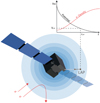 |
Fig. 1. Sketch showing the effect on electron density at the Langmuir probe (LAP1) position from the electrostatic field from the (negative) spacecraft potential that envelopes the sensor. Equipotentials of the electrostatic potential field in the same plane as LAP1 and the spacecraft centre are visualised as concentric blue circles. |
We structure this paper as follows. After a brief description of the instruments used in this study in Sect. 2, we describe the spacecraft potential as measured by LAP and how we can verify that measurement using the attracted ions observed by the ICA in Sect. 3. In Sect. 4, we then show how the spacecraft potential obstructs some of the LAP measurement modes, as well as how we can use the spacecraft potential to our advantage to recover electron densities via cross-calibration and in a similar fashion cross-calibrate the LAP ion currents to electron densities. We thereby obtain a dataset that combines the dynamic range and high resolution of LAP with the accuracy of the MIP. Finally, we present a side effect of the physical model of the cross-calibration routine, which yields accurate estimates on the ion flow speed and EUV flux and agrees with independent measures and previously published results.
2. Instrument description
The Rosetta plasma consortium included, among other instruments, the Rosetta dual Langmuir probe instrument (LAP), which consists of two 5 cm diameter spherical electrostatic probes, LAP1 and LAP2, and their associated electronics. The primary parameter measured are the currents flowing to (or the voltage of) the probes when some bias voltages (or bias currents) are applied to it. From these measurements we can derive plasma characteristics such as plasma density, electron temperature, ion flow speed, as well as spacecraft potential, extreme ultraviolet (EUV) flux, and electric field fluctuations. Not all parameters are monitored simultaneously or uniformly over the mission, as it is contingent on the bias voltage or current (i.e. the operational mode) selected for each probe, and, ultimately, the science objective of each operational period. LAP1 and LAP2 are situated at the ends of separate booms of length 2.24 and 1.62 m, respectively, and are described in further detail in Eriksson et al. (2007).
The Mutual Impedance Probe (MIP), is an active electric sensor that allows us to derive the plasma density via the identification of the plasma resonance frequency. The MIP consists of two pairs of transmitting and receiving electrodes (as well as their associated electronics) and measures the electric coupling of the electrodes to the plasma by fluctuating a charge on the transmitters. The MIP is mounted on a 1 m long bar on the same boom as LAP1, but it can also make use of the LAP2 sensor for transmission, situated ∼4 m away on the LAP2 boom. The MIP is described in further detail by Trotignon et al. (2007).
The Ion Composition Analyzer (ICA) is a mass-resolving ion spectrometer mounted on the Rosetta spacecraft body and included in the RPC package. The ICA has a maximum energy range of a few eV to 40 keV, which it typically sweeps every 12 s with a typical energy resolution of dE/E = 0.07, as well as an angular field of view of 360 × 90 deg (Odelstad et al. 2017; Nilsson et al. 2017). As positive ions are accelerated into the ICA instrument when the spacecraft potential is negative, we can also estimate the spacecraft potential from the measured energy of the lowest energy ions, as described in Odelstad et al. (2017).
3. Spacecraft potential
The spacecraft potential, VS, is fundamental to the interpretation of plasma data. As documented in detail by Odelstad et al. (2015, 2017), LAP uses two complementary techniques of estimating the spacecraft potential. One involves identifying the photoelectron knee potential Vph from a probe sweep, which is the negative of the potential where the probe is in equilibrium with its immediate plasma surroundings and is neither attracting nor repelling photoelectrons emitted from the probe surface. The other method involves measuring the floating potential Vf, which is the negative of the potential for which the sum of all currents to the probe is zero. When LAP is operating in floating potential mode, we measure Vf directly, but we can also estimate it from a sweep (Fig. 2), in which case we denote this parameter Vz.
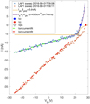 |
Fig. 2. Two example LAP sweeps from 1 Sep 2016 blue and red stars) showing significant spacecraft charging, as well as a visualisation of a selection of parameters from the analysis: the spacecraft potential estimate from the zero-crossing potential; Vz from each sweep (blue and red dots, respectively); the estimated photoemission current for the first sweep (yellow line), which has a discontinuity at Vph (black triangle); the ion current slope fits (green and red dashed lines); and the total current fit to the first sweep (purple solid line). As the spacecraft charging is significant, the electron current is poorly constrained by the bias range, but it is here modelled using a double Maxwellian distribution with characteristic energies of 0.1 eV and 1.5 eV. |
In an ideal scenario, Vz and Vf would be fully equivalent. However, the sweep has a discrete step size, 0.25 or 0.5 V in most modes, and Vz has to be found by interpolation or fitting. Therefore, Vz usually exhibits more noise than Vf, which is also immune to a displacement current added by any capacitive effects when varying the bias voltage. Nevertheless, the method of fitting Vz can increase the range of the estimate by extrapolating beyond the sweep bias voltage window, as shown in Fig. 2. In one of the two sweeps in this example, Vz falls just outside the bias range of the sweep, but as we show below, the extrapolation can reach much further. For sweeps with disturbances (noise or otherwise), there can be several zero-crossings of current. In these cases, each zero-crossing is ranked in descending order of longevity (i.e. the distance to the next zero-crossing in either direction), as we expect disturbances to be short-lasting over sweep timescales. Only the best ranked zero-crossing is chosen for the Vz estimate.
In Fig. 3, we show a validation of the automatic identification of Vz, beyond the sweep range and in comparison to Vf and ICA spacecraft potential estimates. No obvious discontinuities are seen between the two methods in Fig. 3. Statistically, as LAP alternated between continuous floating potential mode and sweeps (yielding Vf and Vz estimates, respectively) over the entire mission, we find a slight shift with a median of 0.4 V and a median absolute deviation of 1.7 V, when we move from one mode to the other.
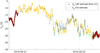 |
Fig. 3. Spacecraft potential estimates from LAP and ICA. Coloured circles are the spacecraft potential estimates from LAP, coloured according to data source. Red circles are derived from Vf. Yellow, blue, and green circles are all derived from Vz, but green indicates values that are extrapolated beyond the sweep range and blue indicates sweeps with several zero-crossings (i.e. disturbances). The blue line is a −3.8 V offset-corrected ICA estimate derived from the negative of the lowest energy bin with at least five ion detections and filtered using a 50-point moving average. We note that there are no obvious discontinuities in moving from Vz to Vf. |
How Vph and Vf relate to the spacecraft potential was studied in detail in Odelstad et al. (2017) whenever we computed simultaneous and good quality estimates from the offset of low-energy ions in the ICA for a spacecraft that is sufficiently negatively charged. Over the entire mission, Vph and Vf diverge slightly as the spacecraft potential approaches zero or becomes slightly positive, with Vf becoming non-linearly less sensitive to spacecraft potential changes, as shown in Fig. 4. Also, the method of detection for Vph relies on the identification of the peak of the second derivative, in other words, the discontinuity of the photoelectron current and, as such, relies on a very good signal-to-noise ratio for an accurate detection. When the signal-to-noise ratio is poor, a Blackman filter (Magnus & Gudmundsson 2008) was applied to the signal before identifying the peak of the second derivative, which can introduce errors and artefacts. However, as Vph relates to the spacecraft potential only by a certain factor (Odelstad et al. 2017), we created an empirical model to map the less noise-sensitive Vf and Vz dataset to equivalent Vph values by use of the fit in Fig. 4. We call this new variable U1 according to
 (1)
(1)
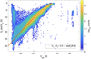 |
Fig. 4. 2D histogram of 390 000 simultaneous spacecraft potential estimates Vph versus Vz or Vf in 200 × 200 bins, corresponding to bin widths of ∼0.3 and 0.5 V, coloured by log10 counts for the entire cometary mission. As Vph is sensitive to noise, there are several artefacts at e.g. +22 V and −25 V, but there is otherwise a clear agreement, especially for large negative values as far as Vph can measure. As the spacecraft potential approaches zero, Vf and Vz diverge non-linearly from Vph, the latter being considered the better estimate for the spacecraft potential at these ranges. An empirical model was fitted to move from Vf and Vz to Vph and is plotted in red. |
where we note that the numerical factors have units of volts and that U1 should be a certain factor α of the spacecraft potential, VS, between 0.7 and 1 according to Odelstad et al. (2017). For the LAP VS estimates plotted in Fig. 3, this factor α is taken to be 0.95. With this empirical model, 68% of all U1 estimates fall within 1 V of Vph in Fig. 4.
4. Method
4.1. MIP-LAP cross-calibration
As described in Sect. 2, the RPC included two instruments targeting the bulk plasma properties, LAP and MIP. The Langmuir probe technique used by LAP is very flexible, enabling access to a broad number of plasma parameters including electron density, electron temperature, and ion temperature or flow speed, and it also provided integrated solar EUV flux, spacecraft potential, and electric field measurements. Other advantages are the broad dynamic range in plasma density (see Sect. 6) and the possibility of very high time resolution (down to 53 μs for LAP). However, perturbations from the spacecraft on the plasma at the probe can sometimes be very large, and disentangling variations of density and temperature is not always possible. The mutual impedance technique used by the MIP is entirely different, resting on observing the transmission properties of the plasma for artificially injected oscillating electric fields in the kHz to MHz range when in active mode, or observing natural plasma oscillations when in passive mode. Compared to LAP, dynamic range, maximum time resolution, and resolution in density are all lower, but the MIP also has two major advantages. First, the main resonance frequency identified by the MIP effectively only depends on the plasma density, with very little complication from temperature variations. Second, for the negative spacecraft potential attained by Rosetta in the inner coma, the MIP density value turns out to be insensitive to the spacecraft potential (Wattieaux et al. 2019).
In order to combine the advantages of the two instruments and measurement principles as discussed above, cross-calibrated datasets have been made available on the ESA Planetary Systems Archive1 (Besse et al. 2018). In the following sections, we provide some results of these cross-calibrations as well as some by-products achieved during the process. In principle, the cross-calibration uses the current or voltage measured by LAP and finds a fit of this to available MIP density data points over a certain time period. This fit can then be used either to obtain a plasma density with the high resolution and/or dynamic range of LAP measurements and the robustness of MIP measurements.
The upper panel in Fig. 5 shows a mission-wide 2D histogram of the (32 s average) MIP electron density versus the (32 s average) current measured by LAP1, at fixed negative bias voltage. For a non-illuminated probe, this is mainly the current due to ion collection, proportionally to the plasma density as seen by the points extending down to about 1 nA and extending to the top right corner. However, when the probe is exposed to sunlight, the resulting current cannot be lower than the contribution from photoelectron emission, as seen by the large number of points around 10 to 50 nA. Section 4.3 shows how this contribution can be identified and used for solar EUV monitoring. As described in Johansson et al. (2017), LAP2 has exhibited clear contamination signatures from a capacitive and a resistive layer, and as such is rarely used for current cross-calibration. Nevertheless, when in floating potential mode, there is no electrical response from the contamination layer, and we have excellent agreement between the two probes.
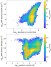 |
Fig. 5. LAP currents in 32-s averages versus simultaneous 32-s average MIP densities over the mission. Top: MIP density versus LAP1 current at negative bias voltage (Vb < −15 V, referred to as ‘ion current’) coloured by log10 counts in each bin. Bottom: MIP density versus LAP1 electron currents (Vb > 20 V) coloured by log10 counts in each bin. |
The lower panel of Fig. 5 illustrates why only currents at negative bias voltage (ion currents) are used for cross-calibration. This 2D histogram shows currents obtained at positive bias voltage with respect to the spacecraft, intended to attract electrons providing a current proportional to plasma density. While some points indeed show the expected correlation, others clearly do not, even exhibiting anti-correlation, and the spread of points is very large. The basic reason for this is the highly negative potential obtained by the spacecraft in high-density plasmas (Johansson et al. 2020), so high that the resulting voltage of the probe can even become negative with respect to the plasma. Such charging is not a problem for the ion current, which maintains a good correlation to the MIP plasma density. This also lends observational support to the insensitivity of the MIP electron density to the spacecraft potential as found by Wattieaux et al. (2019).
We note here that the spacecraft potential, MIP electron density estimates, and LAP currents are all measures of plasma parameters on slightly different spatial scales. The currents to the 5 cm diameter Langmuir probe mainly depend on the plasma within about one metre from the probe2 and therefore is the most local estimate, while the spacecraft potential (derived from currents to a largely conductive spacecraft with a wingspan of 32 m) is the least local. When there are plasma variations on scales below tens of metres, even ideal sets of measurements would only agree in an average sense. As the Debye length in the inner coma typically is ≲1 m (Gilet et al. 2020), such small-scale plasma variations are fully possible, meaning that the scatter observed when comparing, for example, LAP current to MIP plasma density is not necessarily due to measurement uncertainties.
4.2. Cross-calibration of spacecraft potential to electron density
The MIP identifies the electron density via detection of the plasma frequency. Typically, every 1.4−4.3 s, an oscillating electric field is injected in the plasma at stepped frequencies through different electric transmitters. The electric potential that propagates in the plasma is simultaneously measured on the two MIP receivers, from which the complex (amplitude and phase) mutual impedance spectra is built. Eventually, the resonance observed in the mutual impedance spectra at the plasma frequency enables us to retrieve the electron density at a cadence of 0.24−0.74 Hz.
There are two fundamental operational modes of MIP, namely the SDL and LDL modes, used intermittently for smaller and larger Debye lengths, respectively. Therefore, the density targeted by the MIP instrument is limited to two different ranges, and as such, on the selection of a suitable operational mode based on the predicted density days or weeks in advance. It is therefore not surprising that there are intervals in the cometary mission where the electron density falls outside of the MIP sensitivity range (see Sect. 5, Fig. 9). Thus, special care has to be taken when the average density is outside the measurement range but the dynamic variations of the plasma allow the MIP to sporadically detect the lower or upper edge of the density range. If a MIP sample (i.e. a positive MIP plasma resonance identification) is not adjacent to multiple positive identifications (at least five within the ten closest identifications), the MIP sample is disregarded for cross-calibration.
The spacecraft potential is the potential for which the sum of all currents to the spacecraft is zero. Defining a positive current as the flow of positive charges from the spacecraft, the dominating positive and negative current contributions for Rosetta are the cometary electron current and the photoemission current, respectively. In such a plasma, for a negative and conductive spacecraft, VS becomes (Odelstad et al. 2017)
 (2)
(2)
where n is the number density of the electrons, which are assumed to be a Maxwellian population of characteristic temperature Te, given in eV, and C is a constant not depending on plasma properties.
We therefore expected the spacecraft potential to be much more sensitive to the temperature of these electrons than to the electron density. In a recent study (Johansson et al. 2020), we showed that this is not the case and also presented a detailed model explaining why the Rosetta spacecraft potential is sensitive to the density of electrons, regardless of temperature, allowing even cold (0.1 eV) electrons to reach a spacecraft that is often charged from −10 to −20 V. The primary reason is the presence of exposed positively biased conductors on the front-side edges of the solar panels.
As several studies (Heritier et al. 2017a; Breuillard et al. 2019; Johansson et al. 2020) show, and as is visible in Fig. 6, there is a strong relation between the logarithm of the electron density and the spacecraft potential proxy U1. This relation is even more evident over shorter time windows (shown in Fig. 7) as the photoemission current, which is included in C in Eq. (2), can be assumed to be constant. As the orbital parameters are not uniform over the entire mission, some branching is evident in the mission overview in Fig. 6 at the lowest densities, which Rosetta only visited over a selection of heliocentric distances, and thus specific ranges of photoemission current.
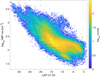 |
Fig. 6. Mission-wide 2D histogram of MIP density versus simultaneous LAP spacecraft potential proxy U1 in 100 × 200 bins coloured by log10 counts. The upper sensitivity limit of MIP in LDL mode is just below 300 cm−3 and is visible as a partial cut-off. |
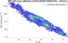 |
Fig. 7. Example of the sliding cross-calibration window. 2D histogram of MIP density versus U1, 50 × 50 bins coloured by counts. The orthogonal least-squares fit (black line) yields an electron temperature of 5.85 eV for 1.053U1 = VS, as per Fig. 3. |
The spacecraft potential is therefore clearly a good proxy for the electron density, and we relate the two in a similar fashion to Breuillard et al. (2019) by rearranging Eq. (2):
 (3)
(3)
where P1 and P2 are both constants over the time interval. P1 is defined as P1 = αkBTe/e, with the definition of α from Sect. 3.
The cross-calibration of electron density to simultaneous U1 estimates was performed with a three-day window that is stepped in one-day steps over the entire mission according to Eq. (3), with some outlier removal, as specified in RO-IRFU-LAP-XCAL3. This rather long calibration window ensures a physical interpretation of each fit, allows us to bridge longer gaps in MIP data, and generates a continuous and mission-wide electron density estimate at the time resolution of the LAP U1 estimate. The dynamical range is also much improved both above and below the sensitivity range of the MIP regardless of its operational mode. Temporal solar EUV events, or rapid and significant fluctuations in electron temperature, will not be correctly captured by the model, but the general trend in the electron density data will still be valid.
4.3. Cross-calibration of ion current to electron density
In a similar but more straightforward fashion, one can relate the ion current to the ion density, and by argument of quasi-neutrality, the electron density (under the assumption that charged cometary dust does not contribute much to the overall current balance). At the bias potentials considered (Vb ≤ −15 V), the Langmuir probe is repelling electrons, such that the current contribution from plasma electrons can be assumed to be negligible, including secondary emission from electron impact. Whenever cometary cold ions are present in the ICA data, they appear supersonic, that is, the thermal speed of ions is much lower than their flow speed (Bergman et al. 2021). This is also supported by the identification of a cometary ion wake behind the spacecraft as discussed in Odelstad et al. (2018). It can be shown (Sagalyn et al. 1963; Fahleson 1967) that for a supersonic flow of ions in a plasma (a cold ion beam), the current to a sunlit probe attracting ions is given by
 (4)
(4)
where Iph0 is the photosaturation current of the probe, defined to be negative, rp is the radius of the probe, Ei is the energy of ions of charge qi and mass mi, and Vp is the absolute potential of the probe according to Vp = Vb + VS. In this cold ion limit, we neglected the thermal velocity component, and we define the effective ion speed ueff, i such that  . For a warm flowing ion plasma, Ei may instead be interpreted as a typical ion energy, combining the thermal and ram energies. A factor of 4/π then appears inside the square-root term in Eq. (4) (Lindqvist et al. 1994), but the linearity of the current-voltage relation remains for all attractive probe potentials (Mott-Smith & Langmuir 1926; Fahleson 1967).
If we assume that the plasma density varies much faster than the ion energy and the EUV flux (and therefore, Iph0), and we ignore small perturbations arising from probe potential variations, we can expect a linear relation between I− and the electron density.
This is shown in an example cross-calibration window in Fig. 8, where the x-intersect yields the photosaturation current. In a similar fashion to what is described in Sect. 4.2, we performed a linear orthogonal least-squares fit of coinciding I− measurements and MIP electron density estimates over a window spanning three hours, which is stepped with one hour over the entire cometary mission. If there are several I− measurements during a MIP density sampling interval, an average is taken. Measurements of I− for a shadowed probe are analysed separately, assuming I−(n = 0) = 0. Some outliers are removed according to RO-IRFU-LAP-XCAL3.
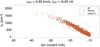 |
Fig. 8. Example of the sliding cross-calibration window for ion current: MIP density versus I− for three hours around 2016-05-23T23:30:00. A linear orthogonal least-squares fit yields an effective ion speed of 9.85 km s−1 and an estimate for Iph0 of −6.92 nA. |
During periods with low electron density and few coinciding MIP and LAP data points (before 1 Jan 2015 and during the so-called night-side excursion around 1 Apr 2016), where no electron density estimates would otherwise be produced, the calibration instead considers a combined dataset of MIP and LAP sweep densities (obtained from fits as in the example in Fig. 2) for the cross-calibration. In this case, the cross-calibration is applied over a larger calibration window (15-day window, five-day step size) to improve the fitting performance. As the spacecraft potential is low or positive during these periods, the reliability of the LAP sweep electron density estimates is considered to be the best available, although still sensitive to electron temperature variations.
5. Results
The performance of the ion current cross-calibration procedure can be seen in Fig. 9. Here, we recover densities in periods where the MIP does not produce electron densities, and (bottom) the temporal resolution has increased dramatically, but is well in agreement with MIP density estimates whenever available.
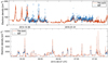 |
Fig. 9. Two examples that illustrates the performance of the cross-calibration. Top: 31 Dec 2014, when the MIP instrument (blue dots) was occasionally in a measurement mode that is not sensitive to low densities, but LAP1 was continuously measuring spacecraft potential, and recovers the density via cross-calibration to spacecraft potential (red line). The errors in the cross-calibration are dominated by uncertainties in the MIP and are typically 25% in both datasets. Bottom: time resolution of the electron density dataset is also improved, here via a ∼60 Hz ion current cross-calibration as described in Sect. 4.3. |
For comparison and as a mission overview, we plot a histogram of the resulting cross-calibrated plasma density datasets, as well as the MIP density, in Fig. 10. The cross-calibrated datasets cover a wider dynamic range of densities, at least for the ion current, and for density ranges fully within the range of the MIP sensitivity we see a near constant ratio between the two datasets, as is expected for two comparable measures with unequal temporal resolution. Also as expected, the ratio drops at the lower edge of the MIP sensitivity range. As noted at the end of Sect. 4.2, the ion current, the MIP density, and the spacecraft potential are all measures on slightly different spatial scales. And even though there is no obvious reason why the density estimates from the spacecraft potential method has an upper limit, estimates above 3000 cm−3 on this (32 m) scale seem rare with this method, and they are instead most common on Langmuir probe current scales. A feature perhaps indicative of the sizes of the plasma structures that move past the Rosetta spacecraft.
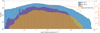 |
Fig. 10. Mission-wide histograms of electron density from the cross-calibration of LAP ion current to the MIP in blue bars, of spacecraft potential to the MIP (purple), and the MIP densities are shown in yellow bars. Also plotted on the axis to the right is the fraction of MIP counts to MIP-LAP I− counts in each density bin. As the LAP current measurement has finite resolution, fractional errors exceed unity below 5 cm−3 even for a perfect calibration of the ion current to density and are therefore not included. |
The physical interpretation of the cross-calibration coefficients yields an estimate for the photosaturation current Iph0 from the x-intersect of the fit in Fig. 8 as I−(n = 0) = Iph0. This new estimate of Iph0 agrees very well with other methods of obtaining the photoemission current published in Johansson et al. (2017), as shown in Fig. 11.
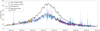 |
Fig. 11. Photosaturation current estimates during the cometary mission from the cross-calibration of ion current to MIP (purple dots) with an associated error bar from the fit of less than five percent; three different photosaturation current estimates are as described in Johansson et al. (2017), where blue and yellow are two out of three independent estimates from LAP with associated error bars; and the black line is a (flare-removed) photosaturation estimate as measured from an EUV monitor at Mars orbit. Also plotted is a low-pass (1/f < 9.5 days) filtered profile of all photosaturation estimates from LAP (red line). |
For the slope coefficient of the ion current cross-calibration fit (dI/dn), we can solve for the effective ion speed via Eq. (4), assuming the spacecraft potential fluctuation is small compared to Vp and that ions are singularly charged with a mass of 19 amu (Heritier et al. 2017b). The resulting speed is plotted in Fig. 12 and compared with a sweep derived ion speed estimate (dI/dV), where we evaluate the slope of the ion current dI/dVb using a linear orthogonal least square fit (see Fig. 2), as well as a coinciding MIP density measurement, as described in detail in Vigren et al. (2017). Random errors are estimated from the uncertainty in the least-squares fits, assuming the errors are normally distributed, and is dominated by MIP sweep frequency discretisation. As the number of MIP and LAP measurement points are much greater in the cross-calibration window than in the sweep estimates, we try to reduce the random errors in the sweep estimates by binning the data in 500 bins of equal length (19 h) over the entire mission.
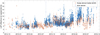 |
Fig. 12. Effective ion speed estimates from the slope of the ion current, dI/dVb, from Langmuir probe sweeps (median of 19 h bins plotted in red) and from dI/dn using three hour-long ∼60 Hz ion current cross-calibration windows (blue). Both methods are using coinciding plasma density estimates from MIP. |
6. Discussion
Before discussing the implications of the cross-calibration, where we focus on the ion-current cross-calibration, we first discuss error sources.
6.1. Errors
In the cross-calibrated densities, the random errors associated with the uncertainty of the associated LAP measurement is very small, typically 5 cm−3, assuming an ion velocity of 5 km s−1. However, the standard error in the calibration is dominated by the uncertainty of the associated MIP measurement (typically 25%), but it is also influenced on the fluctuation of the EUV flux to the probe (if sunlit) or the spacecraft during the calibration interval (typically less than 2 nA and much less than 10%). The final fractional error (assuming the errors are normally distributed) is the sum of the squares of the fractional errors; the error margins of the MIP and the cross-calibrated densities are more or less identical; and for the comparison in Fig. 9 we plot all datasets without the ≈25% fractional uncertainties.
Systematic errors arise from the limited validity of the underlying assumption that the ion density at the probe position is equal to the electron density MIP measures, and at least proportional to the average electron current to the spacecraft, which is an error we cannot easily quantify. If this assumption is not correct, the slope in the fit, and therefore the effective velocity of the ions we estimate from the ion current cross-calibration, should diverge from the true value by some factor equal to the difference in ion and electron densities during the calibration interval. Such effects include sheath effects from the spacecraft potential for ions, and may require further investigation with spacecraft-plasma interaction simulations. However, we can test the assumption by comparing the effective velocity estimate to ICA ion measurements, and we describe this process in Sect. 6.3.
If the ion velocity (for the ion current cross calibration) or the electron temperature of the thermal electron population that dictates the spacecraft potential dependence on electron density (Johansson et al. 2020) is not constant during the cross-calibration interval, errors would grow, and the resulting fit would be poor. Effective ion velocities and photoemission currents resulting from fits with correlation coefficients under 0.7 have therefore been removed.
It should also be noted that the ion current to a Langmuir probe from ions with a superposition of velocity distributions is the superposition of the current from each velocity distribution. Although a Maxwellian simplifies the interpretation of the LAP effective ion speed, it is not dependent on a Maxwellian assumption. The equations that govern the cross-calibration and the ion speed estimates rely on orbital motion limited (OML) theory, in other words, on the assumption that the Langmuir probe size (5 cm) is much smaller than the Debye length, which is generally true for the entire mission (Gilet et al. 2020; Wattieaux et al. 2020). If the Debye length is at any point smaller than the probe size, in very cold and dense plasmas, we note that OML theory yields an upper limit on the collected current. In such cases, we would expect to see more points above the linear trend in Fig. 8 when the density is high, which we generally do not. Similarly, it would yield a significant underestimation of the photoemission when the density is high, but this is not observed in Fig. 11. Additionally, if the thermal velocity is the dominant component of the velocity, in contrast to the findings in Odelstad et al. (2018) and Bergman et al. (2021), our cold ion approximation in Eq. (4) would lead to an overestimation of ueff, i by 13%.
6.2. EUV intensity
We are able to resolve the solar sidereal rotational period of ∼26 days in our photosaturation current from the cross-calibration plotted in Fig. 11, and we also obtain a good agreement with other photosaturation estimates from LAP (of which the shadow-crossing method is believed to be the most accurate). Therefore, we find this result to be another confirmation of the results published in Johansson et al. (2017), as well as of the physical model behind the cross-calibration.
We also note that if there is a significant amount of higher energy (> 20 eV) electrons, such as the population giving rise to electron-impact ionisation in the cometary plasma, this population would also be able to excite and emit secondary electrons from the probe surface. For Cassini in the Saturn magnetosphere, Garnier et al. (2012) found such secondary emission to be a significant contributor to the Langmuir probe current at negative bias voltage. The source population in this case was identified as electrons with energy in the approximate range of 250−450 eV. As significant electron fluxes in this energy range may also have been detected by Rosetta (e.g. Clark et al. 2015; Myllys et al. 2019), one may ask if such currents appreciably contaminate our photoemission estimates. If the secondary yield is higher than one (i.e. more than one electron emitted per incoming high energy electron), then this would constitute an additive offset in all LAP measured Iph0 estimates. However, the shadow-crossing method is insensitive to this secondary emission, except in the highly unlikely case of the electron flux being parallel to the direction from the Sun. The good agreement between the shadow-crossing method with other LAP estimates, whenever available, suggests that secondary electron emission due to impact of high energy electrons generally has little to no effect on our results.
6.3. Effective ion speed
The ion speed estimate from the cross-calibration generally agrees very well with the sweep-derived ion speed in Fig. 12 and again confirms the validity of the physical model in the cross-calibration. They are also very much in line with the average flow velocities as reported by ICA (Nilsson et al. 2020), also during the events investigated in detail by Bergman et al. (2021) as well as previously published LAP estimates (Vigren et al. 2017; Odelstad et al. 2018). Since the two velocity estimates in Fig. 12 arise from two different methods (dI/dVb vs dI/dn), where the internal instrumental offsets are very different (as one involves stepping voltages with the LAP bias circuitry), we conclude that we have a very good grasp of instrument calibration and (as all Iph0 estimates agree) a near-zero contamination on LAP1.
However, for the entire cometary mission, the ion speed estimate is much larger than the neutral velocity of 0.4−1 km s−1 (Hansen et al. 2016) and thus speaks against the assumption made in previous ionospheric models (Heritier et al. 2017a, 2018; Galand et al. 2016) at large heliocentric distances, that ions are flowing with the neutral gas speed. This assumption is not strictly necessary for such ionospheric model density result, and we note that to reconcile our ion speed estimate with these models, either the radial velocity of ions is not the dominant component of the ion flow, or there has to be some mechanism that increases ionisation between Rosetta and the comet nucleus.
As LAP cannot resolve ion density independently, we note that any spacecraft sheath related effects that alter the ion density at the probe location would affect both LAP estimates equally. Validating the ion density with ICA over the entire mission is not currently feasible, mainly due to the limited and distorted field of view (Bergman et al. 2020a,b), such that the ion density estimate would differ from the expectation value at any time, depending on geometry and ion flow direction. However, this has a very limited effect on the ICA ion speed estimate (Bergman et al. 2021). Except for an ion beam that is invariably outside of the ICA instrument field of view during the entire Rosetta mission, we see no reason why the cometary bulk ion speed should be systematically incorrect after a simple correction for the spacecraft potential.
Therefore, to further cross-validate our result, we plot the two LAP estimates together with the magnitude and the radial component of the ICA < 60 eV H2O+ (or H3O+) bulk drift velocity ( and
and  , respectively) from Nilsson et al. (2020) in Fig. 13 for an interval near the tail-side excursion. The estimates are not perfectly equivalent but should still correlate well with the magnitude of the ICA estimate when available.
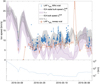 |
Fig. 13. Top: median of 19-h bins of ICA H2O+ ion bulk velocities in terms of magnitude (black line) and a purely radial component (purple line) with corresponding ±1σ spread (shaded) from the standard deviation of the mean, as well as the two LAP effective ion speed estimates from the cross-calibration in Sect. 4.3 (blue line) and 19-h binned medians from sweeps (red line) versus time for a selected time period where the radial distance was rapidly varied. Bottom: radial distance versus time for the same time period. At ∼1000 km to 30 km, the radial component of the ion velocity seems to dominate, and we have good agreement for all estimates when available. Even closer to the comet nucleus, the radial component decreases, perpendicular components grow, and as expected both LAP effective ion speed estimates increase as the magnitude of the velocity increases. |
Here, we find (within error bars) that the radial velocity is dominant and positive at large cometocentric distances (from ∼30 to 1000 km), and increasing with radial distance, which was also noted in the beginning of this interval in Behar et al. (2018). Also, as expected both LAP effective ion speed estimates correlate and agree within error bars with the magnitude of the ICA H2O+ bulk velocity when available, pointing to the existence of a radial electric field such as an ambipolar electric field (Madanian et al. 2016; Vigren & Eriksson 2017; Berčič et al. 2018; Deca et al. 2019). As the ambipolar electric field is proportional to the electron pressure gradient, a radial expansion is consistent with increasing radial ion velocities with cometocentric distance. Moreover, an ambipolar electric field would accelerate electrons falling inward and, as more electrons reach electron-impact ionisation energies, provide increased ionisation between Rosetta and the comet nucleus, as postulated earlier in this section.
As Rosetta moves below 30 km, the radial velocity component decreases, but perpendicular components grow and start to dominate. We suspect that this could again be an effect of an ambipolar electric field as the comet activity is inhomogeneous and bursty by nature, which would create strong non-radial electron-pressure gradients and therefore form an ambipolar electric field with non-radial components. It seems reasonable to expect this field to be strongest near the nucleus, where gas density gradients are great. Also, ions accelerated by a non-radial field close to the comet would also appear radial for a faraway observer with a limited viewing angle resolution. This hypothesis is highly speculative, but could perhaps be tested in the future using simulations similar to those of Deca et al. (2019) and Divin et al. (2020), but resolving the nucleus and allowing for a more realistic outgassing.
This trend also seems generally true for the entire mission, as plotted in Fig. 14, where the combined dataset of the two LAP effective ion speeds, ueff, i, shows large (presumably non-radial) velocities below 30 km from the comet surface. We also find and an acceleration with radial distance beyond 30 km distance, as reported by Berčič et al. (2018) using ICA measurements.
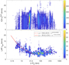 |
Fig. 14. 2D histograms of ion speed versus distance to comet surface coloured by counts, with a common x-axis. Top: radial bulk speed of water ions from ICA, |

Nevertheless, all measured estimates suggest that the ions are moving much faster than the neutrals over the entire mission. The discrepancy between ueff, i and  outside 30 km from the comet surface, although there is overlap, could perhaps be attributed to the fact that the ion density is enhanced at the probe position. If so, the assumption of quasi-neutrality via ne = ni, is incorrect, perhaps by significant electron depletion by dust (Morooka et al. 2011), and would need further investigation. There might also be field-of-view effects on the (mostly nadir pointing) ICA instrument, which warrants further investigation, and is why we, in line with Nilsson et al. (2020), limit our comparison to the radial velocity component in ICA.
If there were a strong bias against ions at lower energies in both ICA and LAP, for instance if the spacecraft potential more easily deflected low-energy ions away from detection surfaces, we would expect there to be a strong dependence on the drift energies on spacecraft potential shown in Fig. 5 in Nilsson et al. (2020), but we find no such dependence. Additionally, as shown in a recent case study by Bergman et al. (2021), there was no indication that there is a significant low-energy cometary ion population present, as detailed spacecraft-plasma interaction simulations of such a environments were incompatible with ICA measurements. Moreover, the instrument field of view increases for low-energy ions on a negatively charged spacecraft (Bergman et al. 2020b), but some uncertainties remain regarding the geometric factor at low ion energies (Bergman et al. 2021). Still, the two LAP estimates, as well as the ICA ion velocity, show elevated ion velocities, for which at least the radial component increases with radial distance. This is consistent with a radial ambipolar electric field that has been predicted to be capable of accelerating the cold newborn ions from the neutral speed to the speed we observe (Vigren & Eriksson 2017).
7. Conclusions
We devised and verified two methods to recover a mission-wide plasma density dataset from the LAP spacecraft potential estimates and the LAP ion current by cross-calibrating the estimate to MIP density whenever available. As a result, we improve the dynamic range as well as the temporal resolution of the RPC plasma density dataset up to a factor of 240 and facilitate plasma analysis on much shorter timescales. The dataset has been made available on the PSA (Eriksson et al. 2020), and at the CDPP on AMDA4. The spacecraft potential and the effective ion speeds resulting from the MIP-LAP ion current cross-calibration model have been successfully cross-validated with ICA, an instrument with a fundamentally different measurement principle.
The physical model that enables the cross-calibration allows for an almost continuous (three-hour cadence) estimate of the effective ion speed and, when the probe is sunlit, the photosaturation current. The latter we find to be well in agreement with independent methods in published studies (Johansson et al. 2017) and to provide support for the conclusions drawn therein regarding attenuation of the EUV.
The ion speed estimates are found to be large ∼5 km s−1 and mostly radial in altitudes above ∼30 km, which is in line with previously published LAP-derived ion speeds (Odelstad et al. 2018; Vigren et al. 2017) and with recent ICA estimates of the ion bulk velocity (Nilsson et al. 2020; Bergman et al. 2021) of H2O+, but in disagreement with the assumption that the ions flow with the speed of the neutrals. This assumption has been made in several modelling works that target plasma densities, and in an average sense successfully reproduce observations at low activity (Vigren et al. 2016; Galand et al. 2016; Heritier et al. 2017a,b, 2018). As a faster radial ion flow would decrease these model density estimates at the Rosetta position, some other error, such as a process that increases the rate of ionisation, must also be present. However, further investigation is needed to confirm that the inferred bulk speeds are representative of the actual drift speed.
The elevated velocity in and of itself points to an electric field present throughout the entire cometary mission, capable of accelerating ions and increasing ionisation via electron impact ionisation between Rosetta and the comet nucleus. Other candidates for the elevated ion speeds (above the neutral speed the ions are born at) includes the wave processes already detected at the comet (André et al. 2017; Ruhunusiri et al. 2020; Karlsson et al. 2017).
The electrostatic field from the Langmuir probe does not reach much farther than the Debye length, but in practice its reach is limited to about one metre, even when the Debye length is longer. This is because the distance at which the vacuum field from a sphere at potential ∼30 V has decayed to the typical energy of the plasma particles collected (∼5 eV) is of the order of 10 probe radii.
Acknowledgments
Rosetta is an ESA mission with contributions from its member states and NASA. This work would not have been possible without the collective efforts over a quarter of a century of all involved in the project and the RPC. This research was funded by the Swedish National Space Agency under grant Dnr 168/15. The cross-calibration of the LAP and MIP data was supported by ESA as part of the Rosetta Extended Archive activities, under contract 4000118957/16/ES/JD. Work at LPC2E is also supported by CNES. We acknowledge the staff of Centre de Données de la Physique des Plasmas (CDPP) for the use of Automated Multi-Dataset Analysis (AMDA). We also acknowledge the ESA Planetary Science Archive for archiving and reviewing the LAP data.
References
- André, M., Odelstad, E., Graham, D. B., et al. 2017, MNRAS, 469, S29 [CrossRef] [Google Scholar]
- Behar, E., Nilsson, H., Henri, P., et al. 2018, A&A, 616, A21 [NASA ADS] [CrossRef] [EDP Sciences] [Google Scholar]
- Berčič, L., Behar, E., Nilsson, H., et al. 2018, A&A, 613, A57 [NASA ADS] [CrossRef] [EDP Sciences] [Google Scholar]
- Bergman, S., Stenberg Wieser, G., Wieser, M., Johansson, F. L., & Eriksson, A. 2020a, J. Geophys. Res.: Space Phys., 125, e2020JA027870 [Google Scholar]
- Bergman, S., Stenberg Wieser, G., Wieser, M., Johansson, F. L., & Eriksson, A. 2020b, J. Geophys. Res.: Space Phys., 125, e2019JA027478 [Google Scholar]
- Bergman, S., Wieser, G. S., Wieser, M., et al. 2021, MNRAS, 503, 2733 [NASA ADS] [CrossRef] [Google Scholar]
- Besse, S., Vallat, C., Barthelemy, M., et al. 2018, Planet. Space Sci., 150, 131 [CrossRef] [Google Scholar]
- Breuillard, H., Henri, P., Bucciantini, L., et al. 2019, A&A, 630, A39 [NASA ADS] [CrossRef] [EDP Sciences] [Google Scholar]
- Carr, C., Cupido, E., Lee, C. G. Y., et al. 2007, Space Sci. Rev., 128, 629 [NASA ADS] [CrossRef] [Google Scholar]
- Clark, G., Broiles, T. W., Burch, J. L., et al. 2015, A&A, 583, A24 [NASA ADS] [CrossRef] [EDP Sciences] [Google Scholar]
- Deca, J., Henri, P., Divin, A., et al. 2019, Phys. Rev. Lett., 123, 055101 [Google Scholar]
- Divin, A., Deca, J., Eriksson, A., et al. 2020, ApJ, 889, L33 [NASA ADS] [CrossRef] [Google Scholar]
- Edberg, N. J. T., Eriksson, A. I., Odelstad, E., et al. 2015, Geophys. Res. Lett., 42, 4263 [NASA ADS] [CrossRef] [Google Scholar]
- Eriksson, A. I., Boström, R., Gill, R., et al. 2007, Space Sci. Rev., 128, 729 [Google Scholar]
- Eriksson, A. I., Engelhardt, I. A. D., André, M., et al. 2017, A&A, 125, A15 [Google Scholar]
- Eriksson, A. I., Gill, R., Johansson, E. P. G., & Johansson, F. L. 2020, ESA Planetary Science Archive and Nasa Planetary Data System [Google Scholar]
- Fahleson, U. 1967, Space Sci. Rev., 7, 238 [NASA ADS] [CrossRef] [Google Scholar]
- Galand, M., Héritier, K. L., Odelstad, E., et al. 2016, MNRAS, 462, S331 [CrossRef] [Google Scholar]
- Garnier, P., Wahlund, J.-E., Holmberg, M. K. G., et al. 2012, J. Geophys. Res., 117, 10202 [CrossRef] [Google Scholar]
- Gilet, N., Henri, P., Wattieaux, G., et al. 2019, Front. Astron. Space Sci., 6, 16 [CrossRef] [Google Scholar]
- Gilet, N., Henri, P., Wattieaux, G., et al. 2020, A&A, 640, A110 [NASA ADS] [CrossRef] [EDP Sciences] [Google Scholar]
- Hansen, K. C., Altwegg, K., Berthelier, J.-J., et al. 2016, MNRAS, 462, S491 [Google Scholar]
- Henri, P., Vallières, X., Hajra, R., et al. 2017, MNRAS, 469, S372 [Google Scholar]
- Heritier, K. L., Henri, P., Vallières, X., et al. 2017a, MNRAS, 469, S118 [CrossRef] [Google Scholar]
- Heritier, K. L., Altwegg, K., Balsiger, H., et al. 2017b, MNRAS, 469, S427 [Google Scholar]
- Heritier, K. L., Galand, M., Henri, P., et al. 2018, A&A, 618, A77 [NASA ADS] [CrossRef] [EDP Sciences] [Google Scholar]
- Johansson, F. L., Odelstad, E., Paulsson, J. J. P., et al. 2017, MNRAS, 469, S626 [NASA ADS] [CrossRef] [Google Scholar]
- Johansson, F. L., Eriksson, A. I., Gilet, N., et al. 2020, A&A, 642, A43 [NASA ADS] [CrossRef] [EDP Sciences] [Google Scholar]
- Karlsson, T., Eriksson, A. I., Odelstad, E., et al. 2017, Geophys. Res. Lett., 44, 1641 [NASA ADS] [Google Scholar]
- Lindqvist, P.-A., Marklund, G. T., & Blomberg, L. G. 1994, Space Sci. Rev., 70, 593 [NASA ADS] [CrossRef] [Google Scholar]
- Madanian, H., Cravens, T. E., Rahmati, A., et al. 2016, J. Geophys. Res.: Space Phys., 121, 5815 [NASA ADS] [CrossRef] [Google Scholar]
- Magnus, F., & Gudmundsson, J. T. 2008, Rev. Sci. Instrum., 79, 073503 [NASA ADS] [CrossRef] [Google Scholar]
- Morooka, M. W., Wahlund, J.-E., Eriksson, A. I., et al. 2011, J. Geophys. Res., 116, A12221 [NASA ADS] [Google Scholar]
- Mott-Smith, H. M., & Langmuir, I. 1926, Phys. Rev., 28, 727 [CrossRef] [Google Scholar]
- Myllys, M., Henri, P., Galand, M., et al. 2019, A&A, 630, A42 [NASA ADS] [CrossRef] [EDP Sciences] [Google Scholar]
- Nilsson, H., Lundin, R., Lundin, K., et al. 2007, Space Sci. Rev., 128, 671 [NASA ADS] [CrossRef] [Google Scholar]
- Nilsson, H., Stenberg Wieser, G., Behar, E., et al. 2017, A&A, 469, S252 [Google Scholar]
- Nilsson, H., Williamson, H., Bergman, S., et al. 2020, MNRAS, 498, 5263 [NASA ADS] [CrossRef] [Google Scholar]
- Odelstad, E., Eriksson, A. I., Edberg, N. J. T., et al. 2015, Geophys. Res. Lett., 42, 10126 [NASA ADS] [CrossRef] [EDP Sciences] [Google Scholar]
- Odelstad, E., Stenberg-Wieser, G., Wieser, M., et al. 2017, MNRAS, 469, S568 [NASA ADS] [CrossRef] [Google Scholar]
- Odelstad, E., Eriksson, A. I., Johansson, F. L., et al. 2018, J. Geophys. Res.: Space Phys., 123, 5870 [NASA ADS] [CrossRef] [Google Scholar]
- Ruhunusiri, S., Howes, G. G., & Halekas, J. S. 2020, J. Geophys. Res.: Space Phys., 125, e2020JA028100 [CrossRef] [Google Scholar]
- Sagalyn, R. C., Smiddy, M., & Wisnia, J. 1963, J. Geophys. Res., 68, 199 [NASA ADS] [CrossRef] [Google Scholar]
- Taylor, M. G. G. T., Altobelli, N., Buratti, B. J., & Choukroun, M. 2017, Philos. Trans. R. Soc. London A: Math. Phys. Eng. Sci., 375 [Google Scholar]
- Trotignon, J.-G., Michau, J. L., Lagoutte, D., et al. 2007, Space Sci. Rev., 128, 713 [NASA ADS] [CrossRef] [Google Scholar]
- Vigren, E., & Eriksson, A. I. 2017, AJ, 153, 150 [NASA ADS] [CrossRef] [Google Scholar]
- Vigren, E., Altwegg, K., Edberg, N. J. T., et al. 2016, AJ, 152, 59 [NASA ADS] [CrossRef] [Google Scholar]
- Vigren, E., André, M., Edberg, N. J. T., et al. 2017, MNRAS, 469, S142 [Google Scholar]
- Wattieaux, G., Gilet, N., Henri, P., Vallières, X., & Bucciantini, L. 2019, A&A, 630, A41 [NASA ADS] [CrossRef] [EDP Sciences] [Google Scholar]
- Wattieaux, G., Henri, P., Gilet, N., Vallieres, X., & Deca, J. 2020, A&A, 638, A124 [NASA ADS] [CrossRef] [EDP Sciences] [Google Scholar]
All Figures
|
Fig. 1. Sketch showing the effect on electron density at the Langmuir probe (LAP1) position from the electrostatic field from the (negative) spacecraft potential that envelopes the sensor. Equipotentials of the electrostatic potential field in the same plane as LAP1 and the spacecraft centre are visualised as concentric blue circles. |
| In the text | |
|
Fig. 2. Two example LAP sweeps from 1 Sep 2016 blue and red stars) showing significant spacecraft charging, as well as a visualisation of a selection of parameters from the analysis: the spacecraft potential estimate from the zero-crossing potential; Vz from each sweep (blue and red dots, respectively); the estimated photoemission current for the first sweep (yellow line), which has a discontinuity at Vph (black triangle); the ion current slope fits (green and red dashed lines); and the total current fit to the first sweep (purple solid line). As the spacecraft charging is significant, the electron current is poorly constrained by the bias range, but it is here modelled using a double Maxwellian distribution with characteristic energies of 0.1 eV and 1.5 eV. |
| In the text | |
|
Fig. 3. Spacecraft potential estimates from LAP and ICA. Coloured circles are the spacecraft potential estimates from LAP, coloured according to data source. Red circles are derived from Vf. Yellow, blue, and green circles are all derived from Vz, but green indicates values that are extrapolated beyond the sweep range and blue indicates sweeps with several zero-crossings (i.e. disturbances). The blue line is a −3.8 V offset-corrected ICA estimate derived from the negative of the lowest energy bin with at least five ion detections and filtered using a 50-point moving average. We note that there are no obvious discontinuities in moving from Vz to Vf. |
| In the text | |
|
Fig. 4. 2D histogram of 390 000 simultaneous spacecraft potential estimates Vph versus Vz or Vf in 200 × 200 bins, corresponding to bin widths of ∼0.3 and 0.5 V, coloured by log10 counts for the entire cometary mission. As Vph is sensitive to noise, there are several artefacts at e.g. +22 V and −25 V, but there is otherwise a clear agreement, especially for large negative values as far as Vph can measure. As the spacecraft potential approaches zero, Vf and Vz diverge non-linearly from Vph, the latter being considered the better estimate for the spacecraft potential at these ranges. An empirical model was fitted to move from Vf and Vz to Vph and is plotted in red. |
| In the text | |
|
Fig. 5. LAP currents in 32-s averages versus simultaneous 32-s average MIP densities over the mission. Top: MIP density versus LAP1 current at negative bias voltage (Vb < −15 V, referred to as ‘ion current’) coloured by log10 counts in each bin. Bottom: MIP density versus LAP1 electron currents (Vb > 20 V) coloured by log10 counts in each bin. |
| In the text | |
|
Fig. 6. Mission-wide 2D histogram of MIP density versus simultaneous LAP spacecraft potential proxy U1 in 100 × 200 bins coloured by log10 counts. The upper sensitivity limit of MIP in LDL mode is just below 300 cm−3 and is visible as a partial cut-off. |
| In the text | |
|
Fig. 7. Example of the sliding cross-calibration window. 2D histogram of MIP density versus U1, 50 × 50 bins coloured by counts. The orthogonal least-squares fit (black line) yields an electron temperature of 5.85 eV for 1.053U1 = VS, as per Fig. 3. |
| In the text | |
|
Fig. 8. Example of the sliding cross-calibration window for ion current: MIP density versus I− for three hours around 2016-05-23T23:30:00. A linear orthogonal least-squares fit yields an effective ion speed of 9.85 km s−1 and an estimate for Iph0 of −6.92 nA. |
| In the text | |
|
Fig. 9. Two examples that illustrates the performance of the cross-calibration. Top: 31 Dec 2014, when the MIP instrument (blue dots) was occasionally in a measurement mode that is not sensitive to low densities, but LAP1 was continuously measuring spacecraft potential, and recovers the density via cross-calibration to spacecraft potential (red line). The errors in the cross-calibration are dominated by uncertainties in the MIP and are typically 25% in both datasets. Bottom: time resolution of the electron density dataset is also improved, here via a ∼60 Hz ion current cross-calibration as described in Sect. 4.3. |
| In the text | |
|
Fig. 10. Mission-wide histograms of electron density from the cross-calibration of LAP ion current to the MIP in blue bars, of spacecraft potential to the MIP (purple), and the MIP densities are shown in yellow bars. Also plotted on the axis to the right is the fraction of MIP counts to MIP-LAP I− counts in each density bin. As the LAP current measurement has finite resolution, fractional errors exceed unity below 5 cm−3 even for a perfect calibration of the ion current to density and are therefore not included. |
| In the text | |
|
Fig. 11. Photosaturation current estimates during the cometary mission from the cross-calibration of ion current to MIP (purple dots) with an associated error bar from the fit of less than five percent; three different photosaturation current estimates are as described in Johansson et al. (2017), where blue and yellow are two out of three independent estimates from LAP with associated error bars; and the black line is a (flare-removed) photosaturation estimate as measured from an EUV monitor at Mars orbit. Also plotted is a low-pass (1/f < 9.5 days) filtered profile of all photosaturation estimates from LAP (red line). |
| In the text | |
|
Fig. 12. Effective ion speed estimates from the slope of the ion current, dI/dVb, from Langmuir probe sweeps (median of 19 h bins plotted in red) and from dI/dn using three hour-long ∼60 Hz ion current cross-calibration windows (blue). Both methods are using coinciding plasma density estimates from MIP. |
| In the text | |
|
Fig. 13. Top: median of 19-h bins of ICA H2O+ ion bulk velocities in terms of magnitude (black line) and a purely radial component (purple line) with corresponding ±1σ spread (shaded) from the standard deviation of the mean, as well as the two LAP effective ion speed estimates from the cross-calibration in Sect. 4.3 (blue line) and 19-h binned medians from sweeps (red line) versus time for a selected time period where the radial distance was rapidly varied. Bottom: radial distance versus time for the same time period. At ∼1000 km to 30 km, the radial component of the ion velocity seems to dominate, and we have good agreement for all estimates when available. Even closer to the comet nucleus, the radial component decreases, perpendicular components grow, and as expected both LAP effective ion speed estimates increase as the magnitude of the velocity increases. |
| In the text | |
|
Fig. 14. 2D histograms of ion speed versus distance to comet surface coloured by counts, with a common x-axis. Top: radial bulk speed of water ions from ICA, |
| In the text | |
Current usage metrics show cumulative count of Article Views (full-text article views including HTML views, PDF and ePub downloads, according to the available data) and Abstracts Views on Vision4Press platform.
Data correspond to usage on the plateform after 2015. The current usage metrics is available 48-96 hours after online publication and is updated daily on week days.
Initial download of the metrics may take a while.