| Issue |
A&A
Volume 653, September 2021
|
|
|---|---|---|
| Article Number | A95 | |
| Number of page(s) | 11 | |
| Section | The Sun and the Heliosphere | |
| DOI | https://doi.org/10.1051/0004-6361/202039905 | |
| Published online | 15 September 2021 | |
One-dimensional prominence threads
I. Equilibrium models
1
Departament de Física, Universitat de les Illes Balears (UIB), 07122 Palma, Spain
e-mail: jaume.terradas@uib.es
2
Institute of Applied Computing & Community Code (IAC 3), UIB, Palma, Spain
3
Departament de Ciències Matemàtiques i Informàtica, Universitat de les Illes Balears (UIB), 07122 Palma, Spain
Received:
13
November
2020
Accepted:
9
June
2021
Context. Threads are the building blocks of solar prominences and very often show longitudinal oscillatory motions that are strongly attenuated with time. The damping mechanism responsible for the reported oscillations is not fully understood yet.
Aims. To understand the oscillations and damping of prominence threads we must first investigate the nature of the equilibrium solutions that arise under static conditions and under the presence of radiative losses, thermal conduction, and background heating. This provides the basis to calculate the eigenmodes of the thread models.
Methods. The non-linear ordinary differential equations for hydrostatic and thermal equilibrium under the presence of gravity are solved using standard numerical techniques and simple analytical expressions are derived under certain approximations. The solutions to the equations represent a prominence thread, a dense and cold plasma region of a certain length that connects with the corona through a prominence corona transition region (PCTR). The solutions can also match with a chromospheric-like layer if a spatially dependent heating function localised around the footpoints is considered.
Results. We have obtained static solutions representing prominence threads and have investigated in detail the dependence of these solutions on the different parameters of the model. Among other results, we show that multiple condensations along a magnetic field line are possible, and that the effect of partial ionisation in the model can significantly modify the thermal balance in the thread, and therefore their length. This last parameter is also shown to be comparable to that reported in the observations when the radiative losses are reduced for typical thread temperatures.
Key words: magnetohydrodynamics (MHD) / waves / Sun: magnetic fields
© ESO 2021
1. Introduction
A recent survey on longitudinal oscillations in solar filaments carried out by Luna et al. (2018) has provided interesting results about the temporal attenuation of the oscillatory motions. A measure of the attenuation is the ratio of the damping time, assuming an exponential decay, to the period of the oscillation. The mean value of this parameter over 106 small amplitude events (with velocities below 10 km s−1) is 1.75, while for large amplitude oscillations (above 10 km s−1) the 96 events give a mean value of 1.25. This means that typically the oscillations do not last more than two periods. The question that arises is what mechanism produces such strong damping, and several approaches can be used to investigate this problem.
The first approach is to consider that the system is near equilibrium satisfying the energetic balance between radiation losses, thermal conduction, and heating. The model may include the effect of the magnetic field and also the gravitational force. Once the equilibrium is calculated, which is the main motivation of the present work (Paper I), the problem of linear and non-linear waves on these equilibrium configurations can be then addressed (Paper II). Only a few works have focused on the determination of a static equilibrium under thermal balance. Degenhardt & Deinzer (1993) modelled a quiescent prominence assuming balance between heating and radiative losses but ignored heat conduction. These authors found reasonable values for prominence temperatures and densities, but significantly shorter threads were obtained (a similar result was obtained by Milne et al. 1979). The connection with the chromosphere was not included in the model. Later, Dahlburg et al. (1998) demonstrated the role of a dipped geometry to support a prominence condensation against gravity and included a localised footpoint heating to match their solution with a chromospheric layer. Regarding the oscillations Schmitt & Degenhardt (1995) and Rempel et al. (1999) performed a stability analysis of a flux tube model based on the work of Degenhardt & Deinzer (1993) under line-tying conditions. However, in these studies the perturbations were assumed to be adiabatic and therefore no attenuation was reported, although some hints of instability were found. The inclusion of non-adiabatic effects under different boundary conditions will be addressed in Paper II. In addition, the effect of partial ionisation, effective for plasma temperatures below 10 000 K, is not taken into account in the above mentioned studies.
The second approach to investigate thread or prominence oscillations is based on the analysis of a dynamical system that undergoes thermal non-equilibrium. Oscillations are naturally produced in the system and their investigation provides details about the damping processes. Along this line, Luna & Karpen (2012) investigated the oscillations of multiple threads formed in long, dipped flux tubes through the thermal non-equilibrium process previously simulated (Luna et al. 2012). These authors found that the oscillation properties predicted by their simulations are in agreement with the observed behaviour, and that the main restoring force is the projected gravity along the tube where the threads oscillate. Zhang et al. (2012, 2013) modelled impulsive heating at one leg of the loop and an impulsive momentum deposition, which cause the prominence to oscillate. The oscillation damps with time under the presence of non-adiabatic processes and these authors concluded that radiative cooling is the dominant factor leading to damping.
In this paper we follow the first approach. We construct improved static prominence or thread models by considering different forms of the radiative losses under the presence of gravity. The basic conditions to have a temperature minimum at the thread centre are derived, and the possibility of having several condensations along the field line is discussed. The connection of the thread solution with the prominence corona transition region (PCTR) and eventually with a chromospheric layer near the footpoints is also investigated. Partial ionisation is included in the model and its effect on the obtained solutions is studied. The work presented here is the basis of the analysis of the eigenmodes that will be described in Paper II.
2. Basic model
We assume that the magnetic field dominates the plasma and reduce the problem to a one-dimensional thread in which the magnetic field determines the geometry but is not modified by the presence of the thread. The plasma quantities change along the thread, and therefore we concentrate on the forces and equilibrium along the field only. This assumption is valid for prominences embedded in sufficiently strong magnetic fields (e.g. Fiedler & Hood 1992; Hillier & van Ballegooijen 2013; Jenkins et al. 2019). For a model with equilibrium normal to the magnetic field, see for example Ballester & Priest (1989). For simplicity, here we concentrate on a 1D problem and the tube cross-section is assumed to be constant. We adopt a symmetric geometry about the midpoint with a dipped region in the central part, as in Antiochos & Klimchuk (1991), Dahlburg et al. (1998), and Zhou et al. (2014). The definition of the field geometry is given by Eq. (6) of Dahlburg et al. (1998). We denote by g(s) the gravity acceleration parallel to the field line and s the distance along this line (starting at the midpoint of the structure, i.e., the centre of the thread). Three different examples of field geometry investigated in the present work are represented in Fig. 1.
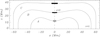 |
Fig. 1. Sketch of the assumed magnetic field geometry. The different parameters change the shape and curvature of the field lines where the thread is allocated (based on Dahlburg et al. 1998). The configurations are labelled A, B, and C. The three configurations are represented with different total lengths for visualisation purposes only. The parameters of each curve following the definition in Dahlburg et al. (1998) are A (bottom curve): s1 = 0.05L, s2 = 0.5L, d = 0.1L; B (middle curve): s1 = 0.1L, s2 = 0.5L, d = 0.05L; and C (top curve): s1 = 0.2L, s2 = 0.5L, d = 0.01L. L is half the length of the magnetic field line. |
3. Fully ionised plasma
For a static situation two equations for the force balance and thermal equilibrium must be satisfied simultaneously. Gas pressure under static equilibrium must satisfy that
When gravity is neglected gas pressure remains constant along s. This equation is completed with the ideal gas law
where kB/mp is the ideal gas constant and  is the mean atomic weight. For a fully ionised hydrogen plasma
  . The modifications in the previous equation because of partial ionisation are introduced in Sect. 4.
Using the ideal gas law we can eliminate the variable p(s) to obtain
For thermal equilibrium between conduction, radiative losses, and heating the next non-linear ordinary differential equation has to be satisfied,
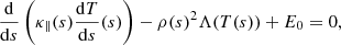
where κ∥(s) = κ0 T(s)5/2, with κ0 a constant coefficient, and Λ(T) is the radiative loss function and E0 the background heating. It is instructive to write the previous energy equation in integral form using the Gauss theorem in one dimension,
![$$ \begin{aligned} \left[\kappa _\parallel (s) \frac{\mathrm{d}T}{\mathrm{d}s}(s)\right]_{s=\pm L}+\int _{-L}^{L}\left(-\rho (s)^2 \Lambda (T(s))+E_0\right)\mathrm{d}s=0, \end{aligned} $$](/articles/aa/full_html/2021/09/aa39905-20/aa39905-20-eq7.gif)
where the first term of this equation represents the (minus) heat flux through the footpoints of the field lines located at ±L and the second term is the spatially integrated contribution of radiation and heating. If E0 is zero the heat flux through the boundaries because of thermal conduction, is equal to the total energy lost by radiation in the whole domain.
For optically thin radiative losses the function Λ(T) has several parametrisations in the literature that are essentially valid for the corona surrounding prominences. Nevertheless, threads are optically thick, and therefore radiative losses are expected to be greatly reduced. This effect can be taken into account by artificially decreasing the values in the optically thin radiative losses for low temperatures (T < 104 K) (see e.g. Milne et al. 1979; Schmitt & Degenhardt 1995). Here we consider two main radiative loss functions, described in Athay (1986) and Hildner (1974), which are represented in Fig. 2 for comparison purposes. Athay’s radiation function has the advantage of being an analytical function with continuous derivatives and attains quite low values under prominence and/or thread conditions. As we show in the next sections, this has important consequences regarding the lengths of the calculated threads. We have explored other radiative losses such as Klimchuk-Raymond’s fits (Klimchuk & Cargill 2001) and the parametrisation computed from CHIANTI atomic database (Dere et al. 1997; Landi et al. 2012), but the results are in general quite similar to those of Hildner’s function.
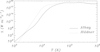 |
Fig. 2. Radiative loss functions used in the present work: Athay (1986) (continuous line) and Hildner (1974) (dotted line). Athay’s function has reduced losses in comparison with Hildner’s for typical temperatures in the range 4000–12 000 K. |
We derive the conditions to obtain a dense and cold thread at the centre of the dip surrounded by a hot plasma. We denote the temperature and density at this point as T0 = T(0) and ρ0 = ρ(0). By symmetry around s = 0 we impose that dT/ds = 0, meaning that Eq. (4) at s = 0 reduces to
Since we are looking for solutions that represent a cold thread connecting with the hot corona, the temperature at s = 0 (where there is an extrema because we have imposed that dT/ds = 0) must have a minimum (i.e., d2T/ds2 > 0). According to Eq. (6), this condition is satisfied only if  . Conditions for the existence of prominence solutions were already studied in some detail in the early work of Milne et al. (1979). We note that even in the unlikely situation with no background heating in the solar atmosphere (i.e. E0 = 0), it is still possible to obtain physically meaningful solutions. However, for
 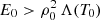 no solutions representative of threads (i.e., cold material surrounded by coronal plasma) are found. Instead, coronal loop solutions of the type studied by Klimchuk et al. (2010) or Mikić et al. (2013), among others, are obtained. The stationary solutions calculated by these last authors by solving the time dependent problem were used as a check of our numerical method based on standard routines. We obtained static equilibrium solutions that closely match the stationary solutions of Mikić et al. (2013).
Typical numbers for background heating found in the literature are in the range 10−4 − 10−5 W m−3 (e.g., Karpen et al. 2001; Mikić et al. 2013); however, for the specific radiative losses considered in this work, these values are in general too high to satisfy the condition  necessary to have a typical thread and/or prominence with density ρ0 = 10−11 kg m−3 and temperature T0 = 10 000 K. For this reason we decided not to focus on a single value of the background heating, but to change the value of E0 in the range between 0 and slightly below
  . It is clear that the value of the radiative loss function at T0 is a relevant number that determines the range of allowed values for E0. If the radiative losses are low for temperatures around 10 000 K the background heating needs to be decreased accordingly. For this reason we consider background heatings as low as E0 = 2.75 × 10⁻⁹ W m−3 and E0 = 1.25 × 10⁻⁶ W m−3 for Athay and Hildner’s radiation functions, but in some cases the values are slightly above these values (e.g. Fig. 3).
 |
Fig. 3. Hydrostatic and thermal equilibrium along the field line with zero gravity. The continuous line corresponds to Athays’s radiation function, the dashed line represents the results for Hildner’s function, while the background heatings are E0 = 2.75 × 10⁻⁹ W m−3 and E0 = 1.75 × 10⁻⁶ W m−3. In this particular example T0 = 104 K, ρ0 = 10−11 kg m−3, and the total length of the field line is 2L = 200 Mm. Model A is used in this plot. |
The system of Eqs. (3) and (4) are solved numerically for T and ρ under given boundary conditions using standard numerical techniques based on a variable-order, variable-step Adams method. At the centre of the thread (s = 0) the temperature (T0) and density (ρ0) values are selected and dT/ds = 0 is imposed. The two coupled ordinary differential equations are numerically integrated from s = 0 to s = L using numerical methods. When necessary, adaptive mesh methods are used, this is especially important at the PCTR. We do not need, in general, to implement a shooting method since the three boundary conditions are imposed at s = 0. The shooting method is only required when density at s = 0 has to be determined to match the temperature at the corona (s = L) (see end of Sect. 3.3). In this last case we use a Runge–Kutta–Merson method and a Newton iteration in the shooting and matching technique.
3.1. Constant gas pressure
For a better comprehension of the results we start with the case of zero gravity. Gas pressure is constant along the field under such conditions, and the solution of the equations is represented in Fig. 3 for the two radiation functions. The solutions show rather different behaviour although the reference temperatures and densities are the same at s = 0. For Athay’s radiation function a single thread around s = 0 is found and matches smoothly through a PCTR a plasma that is close to coronal conditions (densities of the order of 10−13 kg m−3, and temperatures around 106 K). On the contrary, in the case of Hildner’s function, up to three cold and dense regions are found in the configuration. The densities and temperatures of these thread-like solutions are chosen to be exactly the same at the centre of the thread (s = 0). The system displays periodic cold and dense threads; and this behaviour also applies to Athay’s radiation function, but the corresponding spatial periodicity is much longer than the length of the system.
The distance between successive threads depends on the reference values for temperature and density and also on the value of the heating constant. It is clear that for constant gas pressure the system has a characteristic spatial scale and it is worth investigating the origin of this length. It turns out that this scale is closely related to Field’s wavenumber, after Field (1965). This author found that the thermal mode in a uniform plasma with constant temperature of the order of MK is always unstable if thermal conduction is absent. Under the presence of thermal conduction, however, there is a critical length scale that we denote hereafter as LC, for the stabilisation of the thermal mode. In the model used by Field (1965), with uniform temperature and density, the equilibrium satisfies that
and for a given constant pressure value and using the gas law, the density and temperature are obtained from the previous equation, which must be solved numerically in general. Since the equilibrium is isothermal there is no conduction term in Eq. (7), but it is present in the perturbations.
An analysis of the perturbations in this configuration to understand the features of the thermal mode has been done in the past by, for example, Field (1965), van der Linden & Goossens (1991), Soler et al. (2011), and Soler et al. (2012). The obtained dispersion relation shows the existence of a critical length, and that only those perturbations with wavelengths below LC are stable; the expression for LC (see Eq. (26a) in Field 1965) is
Derivatives involving density and radiative losses at constant temperature and constant density are present in the denominator of the previous expression and are evaluated in the second part of the equation where Λ′(T0) is the temperature derivative of the radiative losses evaluated at T0. It is worth mentioning that in Eq. (8) the explicit dependence on E0 is absent, the reason being that in our model the heating only affects the equilibrium but not the perturbations. We note that Begelman & McKee (1990) define a Field’s length which is not the same as the critical length used here (see also Koyama & Inutsuka 2004; Sharma et al. 2010). Begelman & McKee (1990) provide a relationship between the critical and the Field’s length in their Eq. (4.16).
We applied Eq. (8) to the situation in Fig. 3, but we kept in mind that we were comparing the calculated inhomogeneous equilibrium with a model that has constant density and temperature. In order to perform a reliable comparison we chose the same gas pressure value (which is constant along the tube) and the same background heating in the two models. Then we calculated the corresponding density and temperature that satisfies Eq. (7) for the homogeneous model. For example, for the Hildner radiation function we find a temperature of 342 536 K and a density of 2.9 × 10⁻¹³ kg m−3 in the homogeneous model. If we compute the mean values for the corresponding inhomogeneous model (Fig. 3) we obtain a mean temperature of 418 897 K and a mean density of 2.8 × 10⁻¹³ kg m−3; these numbers are similar to those calculated for the homogeneous case. The obtained values of temperature and density for the homogeneous case are introduced in Eq. (8). We find that the corresponding scale length for Hildner radiation function is 36 Mm. This value agrees reasonable well with the periodicity found in Fig. 3 for Hildner’s function, which is around 43 Mm. Repeating the same procedure for Athay’s radiation function (calculating again the temperature and density values) we find that in this case LC = 22881 Mm. This large value explains in Fig. 3 the lack of periodicity in a length of 100 Mm. Therefore, we conclude that the critical length provides a reasonable estimation of the expected periodicity that makes the system stable regarding the thermal instability. Furthermore, we computed different numerical solutions by changing the value of κ0 and positively checked that the obtained characteristic lengths are proportional to the square root of the conduction coefficient, as expected from Eq. (8). We varied other parameters such as temperature and density and the results confirm that Eq. (8) is an adequate approximation. We note that the role of sound waves, and therefore the effect of pressure variations, is absent in the definition of the critical length, while in the full numerical solutions of Fig. 3 the effect of gas pressure is included.
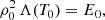
Now we focus on another characteristic scale in the system but of local nature, the length of the individual threads. As we mention in Sect. 1, the calculated lengths by Milne et al. (1979) and Degenhardt & Deinzer (1993) are short in comparison with the measured thread lengths. To investigate this question, and since the dense plasma representing a thread is located around the origin of our coordinate system, we assume that the temperature around s = 0 can be written as a second-order series expansion of the form
where the dimensionless coefficients b1 and b2 need to be determined. Additional terms in Eq. (9) are neglected since s/L ≪ 1 and we perform a local analysis. The boundary condition dT/ds = 0 at s = 0 yields to b1 = 0. For the plasma density we have that using the gas law for constant pressure and in the situation s/L ≪ 1 we can write
We substitute these expansions in s for temperature and pressure in the full energy equation given by Eq. (4). Approximating the powers by the corresponding Taylor series and using again the fact that s/L ≪ 1, we find after some algebra and to zeroth order in s that
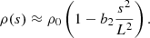
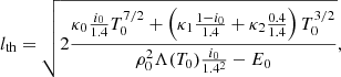
This coefficient is in essence the ratio of the radiative minus the heating term to the conduction term evaluated at s = 0 and assuming that the temperature changes on a spatial scale given by L. Equation (11) provides the value of the term in front of the parabolic dependence on distance, s, in Eq. (9) and it is used here as a proxy to obtain information about the thread length. The smaller the value of b2, the flatter the parabolic curve, and therefore the longer the length of the thread. The question that we have to address is how to define a spatial scale, lth, associated with a parabola. For this reason if we rewrite Eq. (9) as
then
where we use the expression for b2 given in Eq. (11). The spatial scale lth can be understood as an approximation for the thread length, and it provides valuable information about the dependence of this parameter on central density and temperature, radiative losses at this temperature, conduction, and background heating. The radiative losses are dependent on the specific cooling table chosen as this will define the behaviour and therefore shape of the PCTR. Since we are under the assumption  , the parameter lth is always a real positive number. According to Eq. (13) an increase in the conduction will lead to longer threads, while an increase in the radiative losses will shorten them (if E0 is constant). The dependence of lth on the conduction coefficient, κ0, is exactly the same as for LC (see Eq. (8)) although these two spatial scales have different physical meanings. We return to Eq. (13) in the following sections.
3.2. Non-constant gas pressure, gravity included
When gravity is introduced in the system gas pressure is no longer constant along the magnetic field line. We concentrate hereafter on Model A. For large spatial scales we expect that gravity can significantly alter the results in comparison to the constant pressure case, and indeed this is the case. The numerical solution indicates that the second thread solution for Hildner’s function (at s ≈ 45 Mm in Fig. 3) tends to have temperatures much below the minimum at the thread centre (s = 0) and the numerical integration of the equations fails to converge. The system does not allow the periodicity found for the case with zero gravity for the same value of the background heating. In this case no static solution is allowed in the system for the selected parameters and a dynamical behaviour is expected because of the thermal non-equilibrium.
However, by changing E0 it is still possible to find, under some choices of parameters, a situation with two threads under mechanical and thermal balance. An example is shown in Fig. 4. Thus, it is possible to have some cold material in equilibrium balance but not located at the dips. This cold and dense material does not reach the temperature and density values of the central thread, however.
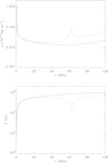 |
Fig. 4. Hydrostatic and thermal equilibrium along the field line with gravity. The continuous line corresponds to Athays’s radiation function and the dashed line represents the results for Hildner’s function, while the background heatings are E0 = 2.75 × 10⁻⁹ W m−3 and E0 = 1.25 × 10⁻⁶ W m−3. In this particular example T0 = 104 K, ρ0 = 10−11 kg m−3 and the total length of the field line is 2L = 200 Mm. Model A is used in this plot. |
In Fig. 4 density and temperature as a function of position along the magnetic field under gravity is also represented for Athay’s function. Interestingly, in this case the differences with respect to the zero gravity situation are not large; essentially the density tends to increase near the footpoint as a result of the presence of gravity since around the footpoint the gravity force is purely vertical and makes the largest contribution (compare with the continuous line in the top panel of Fig. 3). The thread length obtained in this case from the simulations, hereafter denoted as a (do not confuse with lth, the analytical approximation), is 1.7 Mm, and it is calculated using the position where the density derivative with s has a maximum (a is twice this value). We find an extended prominence corona transition region that eventually matches a plasma that is close to coronal conditions (densities of the order of 10−13 kg m−3 and temperatures around 106 K). For these reasons we conclude that the obtained model is a good representation of a thread.
In Fig. 5 the contribution of the different terms in the energy equation is represented for the same parameters of Fig. 4. The conduction term is always positive and is essentially balanced by the radiative losses while the background heating is very small in this example. Both conduction and radiation have a strong peak at the PCTR where density and temperature change abruptly.
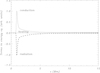 |
Fig. 5. Terms in the energy equation, Eq. (4), as a function of position at the thread body. The continuous line corresponds to the conduction term, the dashed line to the radiation losses, while the dotted line represents the constant background heating. The same parameters as in Fig. 4 for Athay’s function are used. Model A is used in this plot. |
3.3. A parametric survey
Once we know the main features of the solutions we study the influence of the different parameters on the computed equilibrium for a wide range of values. For this reason we carried out a parametric study starting with the dependence on E0. Although from the results in Fig. 5 we can conclude that the role of the background heating is small, it turns out that this parameter has a strong influence on the obtained thread lengths and, as we will show in Paper II, this significantly affects the damping times. This effect of E0 on the equilibrium was already noted by Schmitt & Degenhardt (1995) and is further investigated here.
In Fig. 6 we represent the numerically obtained thread lengths (twice the position where the density derivative with s has a maximum) as a function of E0 for a specific choice of temperature (8 × 10³ K) at the core of the thread. The thread length decreases when the heating is reduced and the minimum thread length is achieved for zero background heating. This agrees with the dependence of lth on  in the denominator of Eq. (13). Analytical approximations for the thread length are more difficult to obtain in this case, but we note that the projection of gravity at s = 0 is precisely zero; therefore, as a first approximation we can still use the definition of lth. The numerical results indicate that the longest thread lengths are obtained for values of the heating tending to the radiative losses at the thread centre, as also expected from Eq. (13). Nevertheless, the analytical approximation given by Eq. (13) and plotted in Fig. 6 with red dashed lines overestimates the thread length in this last situation. It is worth mentioning that there are numerical problems regarding convergence in the calculation of the solutions for values of the heating constant near to
  , but the reason is clear from the denominator of lth.
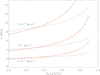 |
Fig. 6. Thread length, a, as a function of the heating constant, E0, for different reference densities ρ0. In this plot the reference temperature is T0 = 8 × 10³ K, and Athay’s radiative loss is used. The analytical approximation given by Eq. (13) is plotted with red dashed lines. Model A is used in this plot. |
We focus now on the dependence of the thread length on the length of the field lines. The three magnetic configurations, denoted by A, B, and C, have been analysed and the total length of the field lines has been changed in the range 80−200 Mm. We found that for Athay’s radiative function the total length of the threads (i.e., the parameter a) does not change much with the length of the magnetic field lines, and the values are typically of the order of several Mm. Interestingly, the thread lengths are in the range reported in the observations (e.g., Okamoto et al. 2007; Arregui et al. 2018). The variation of the thread length with models A, B, and C is at most around 1%. We conclude that the geometry has some influence on the length of the threads, but that it is not too significant. We note that this effect is not included in Eq. (13) since no gravity was assumed in the derivation of this equation (in our model the geometry of the field is only included through the projection of gravity along the magnetic field lines).
On the other hand, when Hildner’s radiative function is considered, the thread lengths are short, typically of the order of only 150 km. Again, the magnetic field geometry has a weak influence on the results in this case. The short lengths of the threads for Hildner’s function were already reported by Milne et al. (1979) and Schmitt & Degenhardt (1995), and the cause is that the radiative losses are too high for typical thread temperatures. On the contrary, Athay’s radiative losses are significantly lower for typical thread temperatures (see the comparison in Fig. 2), and this eventually leads to much longer threads.
In Fig. 7 the obtained thread length is represented as a function of the central temperature for different reference densities. In these calculations we used Athay’s function, and imposed that E0 = 0; therefore, as we have demonstrated in Fig. 6, we concentrate on the shortest threads. Figure 7 indicates that cool threads have longer lengths than hot threads. Furthermore, light threads have larger sizes than heavy threads, which is in agreement again with Eq. (13) (lth is inversely proportional to  ) (see the red dashed lines in Fig. 7).
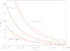 |
Fig. 7. Thread length, a, as a function of the central temperature for different reference densities. The radiative function is based on Athay (1986). The analytical approximation given by Eq. (13) is plotted with red dashed lines. Model A is used in this plot. |
So far we have integrated the ordinary differential equations from s = 0 to s = L because we have imposed three boundary conditions at s = 0 (temperature, density, and zero derivative of temperature), and the problem is well defined. The calculation of the maximum heating is straightforward since it involves the density and temperature at the centre of the thread. Although in some cases we obtained coronal temperatures slightly below 1 MK, in the corona this approach provides reasonable results. However, it is also interesting to investigate the situation where, apart from the thread temperature, the coronal temperature is imposed and the integration provides the rest of the parameters. We are mainly interested in the calculation of the density at the centre of the thread that produces a perfect match for a coronal temperature at s = L. In this case a shooting method is required to solve the differential equations. Now the maximum heating constant is not known since it involves the thread density that has to be determined from the solution of the equations. An iterative approach is required to calculate the maximum E0. To avoid this complication we concentrated on the situation E0 = 0 and studied the dependence of the results on temperature for the three different geometrical configurations. The results are shown in Fig. 8, where the obtained thread densities are plotted as a function of the thread temperatures. The range of thread temperatures for the three configurations agree well with the densities estimated from the observations (e.g., Tandberg-Hanssen 1995; Patsourakos & Vial 2002). The cooler the thread, the higher the density is the behaviour found in the configuration, and is what is expected (using the gas law) from a set of solutions that have essentially the same gas pressure at the centre of the thread. We investigated the situation when the heating constant is different from zero, and again it leads to longer threads than the situation for E0 = 0, as expected from Eq. (13) and demonstrated in Fig. 6.
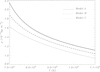 |
Fig. 8. Thread density at s = 0, as a function of the central temperature for models A, B, and C, matching a coronal temperature of 1 MK. A shooting method was used. The radiative function is the same as in Athay (1986). |
3.4. Matching a chromospheric layer
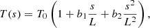
So far we have described a system composed of a cold and dense material representing a thread connecting with a plasma under coronal conditions. A more realistic model should include the connection with the chromosphere near the footpoints of the magnetic field lines that are supposed to be anchored in the photosphere. The physics of the chromosphere is complex and it is beyond the scope of this work to include detailed modelling of this layer. However, it is worth investigating the physical conditions required to have a layer similar to the chromosphere in our simplified 1D system. We have already seen that it is possible to obtain cold and dense plasma regions along the field lines depending on the periodicity of the condensations that can have similar conditions to chromospheric plasmas, especially in the presence of gravity. Nevertheless, these chromospheric regions can occur anywhere along the field line, while we are mostly interested in a chromosphere localised near the footpoints (i.e., near s = ±L in our model). The way to force the coronal part of the previously obtained solutions to match a chromosphere is to include a localised heating source near the footpoints. This approach has been used in the past by several authors and the most common form for the heating function used in the literature is
where λ is a spatial scale typically of the order of 10 Mm and hch is a factor that is in the range 20–100 (see e.g., Dahlburg et al. 1998; Karpen et al. 2001). Using these values in the spatially dependent heating function and solving the ordinary differential equations we obtain a solution with a fast decrease in temperature and a quick increase in density near the footpoint. However, the rapidly changing nature of the chromospheric part of the solution requires, in general, a special treatment of this layer (see Lionello et al. 2009; Johnston & Bradshaw 2019; Zhou et al. 2021 for modifications in the conduction coefficient to avoid such difficulties). Nevertheless, the adaptive methods that are implicitly used in our numerical treatment do not fail to resolve the steep gradients in the solution. It is important to note that the condition  still needs to be satisfied to have a thread-like solution.
The approach used here to incorporate a chromospheric layer in the model is to assume that at some point the temperature remains constant and takes typical chromospheric values (see e.g., Mikić et al. 2013; Karpen et al. 2001). In this situation no energy equation is required, gas pressure must be continuous at this point, and the presence of gravity leads to an exponentially growing density and pressure as we move downwards in the chromospheric part. The integration of the equations is performed from the thread centre to the chromosphere. An example of a computed equilibrium is shown in Fig. 9 for the case hch = 35. In this equilibrium a temperature threshold of 104 K is imposed in the isothermal chromospheric layer, which starts at s = 95 Mm, and its thickness is therefore 5 Mm (larger than the real thickness which is typically around 2 Mm). The exponential increase in density (straight line in the logarithmic scale of the plot) is clear in the top panel of the figure and leads to mean chromospheric density values.
 |
Fig. 9. Hydrostatic and thermal equilibrium along the field line with gravity for Hildner’s function. The background heating is E0 = 5 × 10⁻⁷ W m−3 and hch = 35, 15, 0 for the continuous, dashed, and dotted lines. In this particular example T0 = 104 K, ρ0 = 10−11 kg m−3 and the temperature threshold for the imposed chromosphere is 104 K. Model A is used in this example. |
Using Hildner’s function and for comparison purposes we include in Fig. 9 two solutions with reduced localised heating to visualise the nature of the solutions. For the situations with hch = 15 and hch = 0 we find how temperature decreases near the footpoint, but is still above the temperature threshold (104 K) to have a chromosphere. An interesting conclusion from Fig. 9 is that the presence of footpoint heating does not affect the thread properties and the solution is essentially the same around s = 0 for the three cases. This is also true when Athay’s radiative function is considered. It is worth mentioning that multiple condensations (discussed in Sect. 3.2) are not present in Fig. 9 because the heating constant is always lower than the value used in Fig. 4.
The model developed in this section including a dense and cold chromosphere near the footpoint will be useful for understanding the effect of this layer on the attenuation of the waves (Paper II) produced by the possible mechanism of wave reflection at the chromosphere and wave leakage if the boundary is open.
4. Partially ionised plasma
Let us assume that the plasma is not fully ionised. Based on 1D non-LTE radiative transfer models, Heinzel et al. (2014) calculated, among other parameters, the ionisation degree in several prominence slabs. In particular, Heinzel et al. (2015) provide tables for the ionisation degree for different temperatures and pressures at the prominence. The idea here is to use these values in our calculations of the equilibrium and study how our models are modified by the presence of neutrals. We are again in the situation where the description using an optically thin plasma is not completely correct, but it can be considered a starting point.
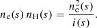
The plasma is assumed to be composed of hydrogen and helium. The abundance of helium is 10% and is not ionised. The ionisation degree is defined here as i = ne/nH where ne is the electron density and nH the total hydrogen density (nHI + np). The total particle number is defined as N = nH + nHe + ne, and using the previous definitions and the helium abundance (nHe = 0.1 nH) it is written as
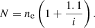
Using the ideal gas law we find that the electron density in terms of pressure, temperature, and ionisation degree is (writing the explicit dependence of the variables)
The ionisation degree, i, depends on p and T and it is calculated from Table 1 of Heinzel et al. (2015). To simplify things, hereafter we write i(p(s),T(s)) as i(s).
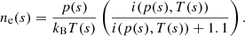
For the total density we have that ρ = nH mp + nHe 4 mp + ne me (being mp and me the proton and electron masses). It reduces to the following expression when the electron mass is neglected in front of the proton mass,
Now the term in the brackets plays the role of  in Eq. (2). In the partially ionised situation it is more convenient to solve the equilibrium equations for gas pressure and temperature because the ionisation degree calculated in Heinzel et al. (2015) depends on these two magnitudes.
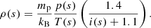
The equation for hydrostatic equilibrium in Eq. (1) is written in terms of pressure and temperature because density has been eliminated using Eq. (17). Partial ionisation changes the equation for thermal equilibrium in the conduction and radiation terms. The factor in front of the radiative term is now
In the conductivities the contribution of neutrals has to be added to the electron contribution. We have that according to Soler et al. (2010, 2012),

where the relative density of species are in our case ξp(s) = i(s)/1.4, ξHI(s) = (1 − i(s))/1.4, and ξHeI = 0.4/1.4. For the conductivities we have that κ0 = 1.1 × 10⁻¹¹ W m−1 K−7/2, κ1 = 2.24 × 10⁻² W m−1 K−3/2, and κ2 = 3.18 × 10⁻² W m−1 K−3/2. The effective conduction coefficient is now the sum of electron and neutral conductivities
The conduction term involves spatial derivatives of this coefficient. The coefficient κ∥ depends on temperature and ionisation degree, and this last parameter also depends on temperature and pressure. Regarding the ionisation, from the practical point of view we adjusted a second-order polynomial to the function i(p, T) given in Heinzel et al. (2015) (table for an altitude of 20 Mm). The calculation of the partial derivatives of i with p and T is straightforward using the polynomial fit.
We repeated some of the previous calculations including the effect of partial ionisation through the change in the radiation and conduction terms and the modification of the ideal gas law. Since we have shown that the inclusion of a chromosphere has little effect on the conditions within the threads, we do not include this pseudo-layer in the present calculations.
The main result is that partial ionisation significantly increases the size of the thread. An example is shown in Fig. 10 where the length of the thread is four times longer than in the fully ionised case. We have to keep in mind that the initial values of the thread parameters at s = 0, required to perform the integration of the differential equations, are now different to those in the fully ionised case because of the change introduced in the gas law by partial ionisation (see Eq. (17)). In the present example temperature and gas pressure are the same at the thread centre, but the reference density is different. In Fig. 10 (bottom panel) we can see how the ionisation degree changes inside the thread because of the implemented model of Heinzel et al. (2015). The ionisation degree raises smoothly from 0.72 at the thread centre to 1 at the edge of the thread where high (coronal) temperatures are achieved.
 |
Fig. 10. Hydrostatic and thermal equilibrium along a thread under partial ionisation (continuous lines) and full ionisation (dashed lines). In this particular example temperature (T0 = 8 × 10³ K) and pressure at (s = 0) are the same for the partially and fully ionised situations. In these solutions E0 = 0 is imposed. The radiative function is the same as in Athay (1986). Model A is used in this plot. |
The increment in the thread length produced by partial ionisation is a consequence of the changes in thermal conduction, which is larger owing to the contribution of neutrals on the conductivities. For a better understanding of this feature we proceed as in the fully ionised situation when gravity is absent. Using the same approximation as in Eq. (9), we find that under the presence of partial ionisation the characteristic spatial scale of the thread is
where i0 = i(p0, T0) is the ionisation degree at the centre of the thread. The value of i0 is typically around 0.72, but the reference density, ρ0, also depends on i0 (see Eq. (17)). It is not difficult to calculate the ratio of the radiation term for partial ionisation relative to full ionisation for constant reference pressure (p0) and temperature (T0). For partial ionisation the reference density is
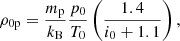
while for full ionisation
The ratio of the two corresponding radiation terms is
This ratio is always lower than one, meaning that radiative losses under partial ionisation are reduced in comparison with the fully ionised case. Since this term appears in the denominator of Eq. (22) it means that it produces an increase in the thread length.
For thermal conduction we need to evaluate the three terms that appear in the numerator of Eq. (22). The sum of the three terms is typically around 4.5 times the value for the fully ionised situation. This increment leads to longer threads under partial ionisation. It turns out that the increased conduction under partial ionisation is mostly produced by the presence of neutral helium. This is visualised in Fig. 11 where the different conduction terms are plotted as a function of position for a typical case. Inside the thread, conduction by neutrals dominates conduction by electrons. The contribution of neutral helium is the largest, although its abundance is just 10%. Conduction by neutral H goes to zero as we approach the edge of the thread where plasma is fully ionised. In the coronal medium the contribution of neutral He is artificially forced to go to zero since at coronal temperatures it is fully ionised. Neutral He is therefore responsible, together with the reduced radiation, for the rise of the obtained thread lengths.
 |
Fig. 11. Conduction terms as a function of position (in the range 0–30 Mm for visualisation purposes). Conduction by neutral H (dashed line) goes to zero at the edge of the thread where the plasma is fully ionised. Conduction by neutral He (dotted line) dominates inside the thread and becomes zero in the corona where there is conduction by electrons only (continuous line). The same parameters as in Fig. 10 are used. |
Finally, Fig. 12 shows how the thread length changes with the central temperature under partial ionisation. The behaviour is the same as in Fig. 7 for the fully ionised case, and for comparison purposes we also represent the results for full ionisation for the same reference pressure at s = 0. Interestingly, as the central temperature increases the two curves approach each other since the higher the temperature, the larger the ionisation degree in the prominence. We find again longer threads in the presence of partial ionisation; the difference is relative to full ionisation, a factor that varies from 5.3 to 2.6 in the range of temperatures of the plot. The analytical approximation given by Eq. (22) is also plotted in the figure, and the agreement with the numerical result is remarkable.
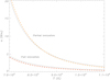 |
Fig. 12. Thread length as a function of temperature under partial ionisation and full ionisation. In these solutions E0 = 0 is imposed. The radiative function is the same as in Athay (1986). The analytical approximations given by Eqs. (22) (partial ionisation) and (13) (full ionisation) are plotted with orange and red dashed lines. The same parameters as in Fig. 10 are used. |
5. Summary and conclusions
In the present work we have analysed the features of one-dimensional equilibrium thread models under hydrostatic and thermal balance. We started with the situation without gravity and progressively increased the complexity of the model. This has allowed us a better comprehension of the results. Gravitational stratification, the presence of a chromosphere, and finally partial ionisation effects were incorporated into our model. The main outcome of our study is summarised in the following:
-
The value of the background heating in comparison with the radiative losses at the centre of the thread is crucial to lead to thread-like solutions surrounded by coronal plasma. Only if
 do static, cold, and dense plasma threads under thermal equilibrium exist. In the opposite situation when the background heating is higher than the radiative losses at the centre of the structure, only loop-like solutions are achieved.
 -
Several thread-like condensations are in principle possible along the field lines and not necessarily located at the dips of the magnetic field. We find that the physical origin of the secondary condensations is related to the critical length introduced by Field (1965) and related to the characteristic spatial scale for thermal stability.
-
The presence of gravity in the model can produce that the secondary condensations collapse and no equilibrium configuration on a given length of the magnetic field line is achieved. Again the value of the background heating plays a major role in the behaviour of secondary thread-like solutions, located in general near the footpoints. The gravitational stability of the obtained solutions needs to be investigated; this will be addressed in Paper II.
-
A parametric survey has been carried out to understand the dependence of the thread length, on the different values of the parameters. The geometry of the field lines is not especially important, but the radiative losses for low temperatures are crucial to obtain realistic thread lengths. Athay’s radiative function, with reduced losses under typical thread conditions (see Fig. 2), is the most suitable choice from the ensemble of radiative losses analysed in the present work. In any case, since the plasma is optically thick under typical prominence and/or thread conditions, the incorporation of more realistic physics requires us to properly solve the radiative transport problem.
-
We have derived a simple analytical expression for the characteristic spatial scale of the thread, lth, under static equilibrium that explains the dependence of the computed thread lengths, a, with the different parameters of the model, including partial ionisation. This could be used in a novel way, for example to infer the ratio of radiation to heating if the length of the thread and the central temperature and density are known from observations.
-
Significantly long threads are obtained when partial ionisation is present. This is a consequence of the reduced radiation and increased conduction produced by neutral helium in comparison to the fully ionised case. It is assumed that helium is totally neutral in the thread, but this is not completely true under real conditions (see Soler et al. 2010), and in reality this may decrease the length of the threads. This needs to be addressed in the future.
-
The connection of the thread-corona system with a chromosphere is obtained when heating around a certain threshold is localised near the footpoints, in agreement with Dahlburg et al. (1998). The chromospheric model used here (a stratified and isothermal layer under full ionisation) is a first approximation, and more physics needs to be included in future studies. However, the presence of a chromosphere is interesting for the applications regarding the damped oscillations that will be discussed in Paper II.
-
Related to the previous point, we have shown that localised footpoint heating does not significantly alter the temperature and density of the cold plasma representing the thread relative to the case without footpoint heating, at least for the parameters considered in this work. In our model the localised heating essentially leads to the existence of a chromospheric layer alone.
The numerical solutions presented in this work will be used to compute the corresponding eigenmodes to compare the damping rates of our calculations and the reported in the observations (Paper II). Firstly, this will allow us to better understand the damping mechanism of the oscillations, and secondly, this information will be used to constrain or to infer some modifications to the models (see Anzer & Heinzel 2008) and most likely about the dependence of the radiative losses on temperature. The comparison of theory and observations will be used for seismological purposes.
Acknowledgments
We acknowledge the support from grant AYA2017-85465-P (MINECO/AEI/FEDER, UE), to the Conselleria d’Innovació, Recerca i Turisme del Govern Balear, and also to IAC3. We are grateful to the ISSI Team led by M. Luna “Large-Amplitude Oscillations as a Probe of Quiescent and Erupting Solar Prominences” for inspiring this work in the fruitful meetings held in Bern in 2018 and 2019. We also thank ISSI-Beijing for hosting the team “The eruption of solar filaments and the associated mass and energy transport” led by J. C. Vial and P. F. Chen where part of the results of this paper were presented. M. Luna acknowledges support through the Ramón y Cajal fellowship RYC2018-026129-I from the Spanish Ministry of Science and Innovation, the Spanish National Research Agency (Agencia Estatal de Investigación), the European Social Fund through Operational Program FSE 2014 of Employment, Education and Training and the Universitat de les Illes Balears. We are grateful to Rafel Prohens from the Departament de Ciències Matemàtiques i Informàtica, Universitat de les Illes Balears (UIB) for his advise on phase analysis of non-linear differential equations. We thank the anonymous referee for their useful comments that helped to improve the manuscript.
References
- Antiochos, S. K., & Klimchuk, J. A. 1991, ApJ, 378, 372 [NASA ADS] [CrossRef] [Google Scholar]
- Anzer, U., & Heinzel, P. 2008, A&A, 480, 537 [NASA ADS] [CrossRef] [EDP Sciences] [Google Scholar]
- Arregui, I., Oliver, R., & Ballester, J. L. 2018, Liv. Rev. Sol. Phys., 15, 3 [Google Scholar]
- Athay, R. G. 1986, ApJ, 308, 975 [Google Scholar]
- Ballester, J. L., & Priest, E. R. 1989, A&A, 225, 213 [NASA ADS] [Google Scholar]
- Begelman, M. C., & McKee, C. F. 1990, ApJ, 358, 375 [NASA ADS] [CrossRef] [Google Scholar]
- Dahlburg, R. B., Antiochos, S. K., & Klimchuk, J. A. 1998, ApJ, 495, 485 [NASA ADS] [CrossRef] [Google Scholar]
- Degenhardt, U., & Deinzer, W. 1993, A&A, 278, 288 [NASA ADS] [Google Scholar]
- Dere, K. P., Landi, E., Mason, H. E., Monsignori Fossi, B. C., & Young, P. R. 1997, A&AS, 125, 149 [NASA ADS] [CrossRef] [EDP Sciences] [Google Scholar]
- Fiedler, R. A. S., & Hood, A. W. 1992, Sol. Phys., 141, 75 [Google Scholar]
- Field, G. B. 1965, ApJ, 142, 531 [NASA ADS] [CrossRef] [Google Scholar]
- Heinzel, P., Vial, J. C., & Anzer, U. 2014, A&A, 564, A132 [NASA ADS] [CrossRef] [EDP Sciences] [Google Scholar]
- Heinzel, P., Gunár, S., & Anzer, U. 2015, A&A, 579, A16 [NASA ADS] [CrossRef] [EDP Sciences] [Google Scholar]
- Hildner, E. 1974, Sol. Phys., 35, 123 [NASA ADS] [CrossRef] [Google Scholar]
- Hillier, A., & van Ballegooijen, A. 2013, ApJ, 766, 126 [NASA ADS] [CrossRef] [Google Scholar]
- Jenkins, J. M., Hopwood, M., Démoulin, P., et al. 2019, ApJ, 873, 49 [NASA ADS] [CrossRef] [Google Scholar]
- Johnston, C. D., & Bradshaw, S. J. 2019, ApJ, 873, L22 [NASA ADS] [CrossRef] [Google Scholar]
- Karpen, J. T., Antiochos, S. K., Hohensee, M., Klimchuk, J. A., & MacNeice, P. J. 2001, ApJ, 553, L85 [NASA ADS] [CrossRef] [Google Scholar]
- Klimchuk, J. A., & Cargill, P. J. 2001, ApJ, 553, 440 [NASA ADS] [CrossRef] [Google Scholar]
- Klimchuk, J. A., Karpen, J. T., & Antiochos, S. K. 2010, ApJ, 714, 1239 [NASA ADS] [CrossRef] [Google Scholar]
- Koyama, H., & Inutsuka, S.-I. 2004, ApJ, 602, L25 [NASA ADS] [CrossRef] [Google Scholar]
- Landi, E., Del Zanna, G., Young, P. R., Dere, K. P., & Mason, H. E. 2012, ApJ, 744, 99 [Google Scholar]
- Lionello, R., Linker, J. A., & Mikić, Z. 2009, ApJ, 690, 902 [CrossRef] [Google Scholar]
- Luna, M., & Karpen, J. 2012, ApJ, 750, L1 [NASA ADS] [CrossRef] [Google Scholar]
- Luna, M., Karpen, J. T., & DeVore, C. R. 2012, ApJ, 746, 30 [Google Scholar]
- Luna, M., Karpen, J., Ballester, J. L., et al. 2018, ApJS, 236, 35 [NASA ADS] [CrossRef] [Google Scholar]
- Mikić, Z., Lionello, R., Mok, Y., Linker, J. A., & Winebarger, A. R. 2013, ApJ, 773, 94 [NASA ADS] [CrossRef] [Google Scholar]
- Milne, A. M., Priest, E. R., & Roberts, B. 1979, ApJ, 232, 304 [NASA ADS] [CrossRef] [Google Scholar]
- Okamoto, T. J., Tsuneta, S., Berger, T. E., et al. 2007, Science, 318, 1577 [NASA ADS] [CrossRef] [PubMed] [Google Scholar]
- Patsourakos, S., & Vial, J.-C. 2002, Sol. Phys., 208, 253 [NASA ADS] [CrossRef] [Google Scholar]
- Rempel, M., Schmitt, D., & Glatzel, W. 1999, A&A, 343, 615 [NASA ADS] [Google Scholar]
- Schmitt, D., & Degenhardt, U. 1995, Rev. Mod. Astron., 8, 61 [NASA ADS] [Google Scholar]
- Sharma, P., Parrish, I. J., & Quataert, E. 2010, ApJ, 720, 652 [NASA ADS] [CrossRef] [Google Scholar]
- Soler, R., Oliver, R., & Ballester, J. L. 2010, A&A, 512, A28 [NASA ADS] [CrossRef] [EDP Sciences] [Google Scholar]
- Soler, R., Ballester, J. L., & Goossens, M. 2011, ApJ, 731, 39 [NASA ADS] [CrossRef] [Google Scholar]
- Soler, R., Ballester, J. L., & Parenti, S. 2012, A&A, 540, A7 [NASA ADS] [CrossRef] [EDP Sciences] [Google Scholar]
- Tandberg-Hanssen, E. 1995, The Nature of Solar Prominences, 199, 308 [Google Scholar]
- van der Linden, R. A. M., & Goossens, M. 1991, Sol. Phys., 134, 247 [NASA ADS] [CrossRef] [Google Scholar]
- Zhang, Q. M., Chen, P. F., Xia, C., & Keppens, R. 2012, A&A, 542, A52 [NASA ADS] [CrossRef] [EDP Sciences] [Google Scholar]
- Zhang, Q. M., Chen, P. F., Xia, C., Keppens, R., & Ji, H. S. 2013, A&A, 554, A124 [NASA ADS] [CrossRef] [EDP Sciences] [Google Scholar]
- Zhou, Y.-H., Chen, P.-F., Zhang, Q.-M., & Fang, C. 2014, Res. Astron. Astrophys., 14, 581 [NASA ADS] [CrossRef] [Google Scholar]
- Zhou, Y.-H., Ruan, W.-Z., Xia, C., & Keppens, R. 2021, A&A, 648, A29 [NASA ADS] [CrossRef] [EDP Sciences] [Google Scholar]
All Figures
|
Fig. 1. Sketch of the assumed magnetic field geometry. The different parameters change the shape and curvature of the field lines where the thread is allocated (based on Dahlburg et al. 1998). The configurations are labelled A, B, and C. The three configurations are represented with different total lengths for visualisation purposes only. The parameters of each curve following the definition in Dahlburg et al. (1998) are A (bottom curve): s1 = 0.05L, s2 = 0.5L, d = 0.1L; B (middle curve): s1 = 0.1L, s2 = 0.5L, d = 0.05L; and C (top curve): s1 = 0.2L, s2 = 0.5L, d = 0.01L. L is half the length of the magnetic field line. |
| In the text | |
|
Fig. 2. Radiative loss functions used in the present work: Athay (1986) (continuous line) and Hildner (1974) (dotted line). Athay’s function has reduced losses in comparison with Hildner’s for typical temperatures in the range 4000–12 000 K. |
| In the text | |
|
Fig. 3. Hydrostatic and thermal equilibrium along the field line with zero gravity. The continuous line corresponds to Athays’s radiation function, the dashed line represents the results for Hildner’s function, while the background heatings are E0 = 2.75 × 10⁻⁹ W m−3 and E0 = 1.75 × 10⁻⁶ W m−3. In this particular example T0 = 104 K, ρ0 = 10−11 kg m−3, and the total length of the field line is 2L = 200 Mm. Model A is used in this plot. |
| In the text | |
|
Fig. 4. Hydrostatic and thermal equilibrium along the field line with gravity. The continuous line corresponds to Athays’s radiation function and the dashed line represents the results for Hildner’s function, while the background heatings are E0 = 2.75 × 10⁻⁹ W m−3 and E0 = 1.25 × 10⁻⁶ W m−3. In this particular example T0 = 104 K, ρ0 = 10−11 kg m−3 and the total length of the field line is 2L = 200 Mm. Model A is used in this plot. |
| In the text | |
|
Fig. 5. Terms in the energy equation, Eq. (4), as a function of position at the thread body. The continuous line corresponds to the conduction term, the dashed line to the radiation losses, while the dotted line represents the constant background heating. The same parameters as in Fig. 4 for Athay’s function are used. Model A is used in this plot. |
| In the text | |
|
Fig. 6. Thread length, a, as a function of the heating constant, E0, for different reference densities ρ0. In this plot the reference temperature is T0 = 8 × 10³ K, and Athay’s radiative loss is used. The analytical approximation given by Eq. (13) is plotted with red dashed lines. Model A is used in this plot. |
| In the text | |
|
Fig. 7. Thread length, a, as a function of the central temperature for different reference densities. The radiative function is based on Athay (1986). The analytical approximation given by Eq. (13) is plotted with red dashed lines. Model A is used in this plot. |
| In the text | |
|
Fig. 8. Thread density at s = 0, as a function of the central temperature for models A, B, and C, matching a coronal temperature of 1 MK. A shooting method was used. The radiative function is the same as in Athay (1986). |
| In the text | |
|
Fig. 9. Hydrostatic and thermal equilibrium along the field line with gravity for Hildner’s function. The background heating is E0 = 5 × 10⁻⁷ W m−3 and hch = 35, 15, 0 for the continuous, dashed, and dotted lines. In this particular example T0 = 104 K, ρ0 = 10−11 kg m−3 and the temperature threshold for the imposed chromosphere is 104 K. Model A is used in this example. |
| In the text | |
|
Fig. 10. Hydrostatic and thermal equilibrium along a thread under partial ionisation (continuous lines) and full ionisation (dashed lines). In this particular example temperature (T0 = 8 × 10³ K) and pressure at (s = 0) are the same for the partially and fully ionised situations. In these solutions E0 = 0 is imposed. The radiative function is the same as in Athay (1986). Model A is used in this plot. |
| In the text | |
|
Fig. 11. Conduction terms as a function of position (in the range 0–30 Mm for visualisation purposes). Conduction by neutral H (dashed line) goes to zero at the edge of the thread where the plasma is fully ionised. Conduction by neutral He (dotted line) dominates inside the thread and becomes zero in the corona where there is conduction by electrons only (continuous line). The same parameters as in Fig. 10 are used. |
| In the text | |
|
Fig. 12. Thread length as a function of temperature under partial ionisation and full ionisation. In these solutions E0 = 0 is imposed. The radiative function is the same as in Athay (1986). The analytical approximations given by Eqs. (22) (partial ionisation) and (13) (full ionisation) are plotted with orange and red dashed lines. The same parameters as in Fig. 10 are used. |
| In the text | |
Current usage metrics show cumulative count of Article Views (full-text article views including HTML views, PDF and ePub downloads, according to the available data) and Abstracts Views on Vision4Press platform.
Data correspond to usage on the plateform after 2015. The current usage metrics is available 48-96 hours after online publication and is updated daily on week days.
Initial download of the metrics may take a while.