| Issue |
A&A
Volume 652, August 2021
|
|
|---|---|---|
| Article Number | A45 | |
| Number of page(s) | 7 | |
| Section | Celestial mechanics and astrometry | |
| DOI | https://doi.org/10.1051/0004-6361/202141344 | |
| Published online | 06 August 2021 | |
Astrometric radial velocities for nearby stars
Lund Observatory, Department of Astronomy and Theoretical Physics, Lund University,
Box 43,
22100
Lund,
Sweden
e-mail: This email address is being protected from spambots. You need JavaScript enabled to view it.
; This email address is being protected from spambots. You need JavaScript enabled to view it.
Received:
19
May
2021
Accepted:
14
June
2021
Abstract
Context. Under certain conditions, stellar radial velocities can be determined from astrometry, without any use of spectroscopy. This enables us to identify phenomena, other than the Doppler effect, that are displacing spectral lines.
Aims. The change of stellar proper motions over time (perspective acceleration) is used to determine radial velocities from accurate astrometric data, which are now available from the Gaia and HIPPARCOS missions.
Methods. Positions and proper motions at the epoch of HIPPARCOS are compared with values propagated back from the epoch of the Gaia Early Data Release 3. This propagation depends on the radial velocity, which obtains its value from an optimal fit assuming uniform space motion relative to the solar system barycentre.
Results. For 930 nearby stars we obtain astrometric radial velocities with formal uncertainties better than 100 km s−1; for 55 stars the uncertainty is below 10 km s−1, and for seven it is below 1 km s−1. Most stars that are not components of double or multiple systems show good agreement with available spectroscopic radial velocities.
Conclusions. Astrometry offers geometric methods to determine stellar radial velocity, irrespective of complexities in stellar spectra. This enables us to segregate wavelength displacements caused by the radial motion of the stellar centre-of-mass from those induced by other effects, such as gravitational redshifts in white dwarfs.
Key words: astrometry / proper motions / techniques: radial velocities / methods: data analysis / white dwarfs
© ESO 2021
1 Introduction
Stellar radial velocities of enhanced precision are required for applications such as the tracing of stellar wobble caused by an exoplanet, motion against a binary companion, or velocity relative to nearby stars in a moving cluster. The common method of interpreting wavelength positions of spectral lines in terms of a Doppler shift caused by radial motion reaches a limit when accuracies much better than ~1 km s−1 are required. Even for objects with well-defined and rich spectra, limits are set by spectral line asymmetries and displacements caused by physical motions on the stellar surface and by gravitational redshifts. One step towards an improved understanding of such effects and their eventual mitigation is to measure stellar radial velocities also without the use of spectroscopy. With adequate accuracy and sufficient baselines in time, such determinations are now enabled through space astrometry.
Astrometric methods to determine the radial component of stellar motion include monitoring the secular change of the annual parallax, measuring changes in proper motion, and assessing the varying angular extent of moving clusters whose stars share the same space velocity (Dravins et al. 1999). Among these methods, the moving-cluster one offered the highest accuracy based on HIPPARCOS data (Perryman et al. 1997), and radial motions for stars in such clusters have been determined by de Bruijne et al. (2001), Leão et al. (2019), Lindegren et al. (2000), and Madsen et al. (2002). When combining astrometric data with spectroscopic data, it then becomes possible to search for phenomena, other than the Doppler effect, that are displacing stellar spectral lines (Lindegren & Dravins 2003; Madsen et al. 2003; Moschella et al. 2021; Pasquini et al. 2011; Pourbaix et al. 2002). In solar-type stars, both convective blueshifts and gravitational redshifts amount to ~0.5 km s−1, while the moving-cluster method enables accuracies of the order of a few hundred m s−1. Such levels are comparable to the modulation of apparent radial velocities by stellar magnetic activity (Meunier 2021).
2 Perspective change of proper motions
In this paper, we examine how perspective acceleration, measured as proper motions changing over time, permits the radial component of stellar motion to be determined. The potential of such astrometric observations was realised already long ago (Ristenpart 1902; Schlesinger 1917; Seeliger 1900); however, except for a few stars of very large proper motion, they were not practical to apply until adequate observational precision was achieved by space astrometry. By combining positions and proper motions from HIPPARCOS with old measurements from the Carte du Ciel and its Astrographic Catalogue, Dravins et al. (1999) obtained astrometric radial velocities for 16 stars with typical errors in the range of 30–40 km s−1. For one object, however, the data could be combined with the visual observations by Bessel from 1838, reducing the uncertainty to 11 km s−1. Recent data releases from the Gaia mission have enabled order-of-magnitude improvements over the past HIPPARCOS study, and they are thetopic of this paper.
Proper motions of stars change gradually with time even if their space motions are strictly uniform relative to the solar system barycentre (SSB). This perspective (or secular) acceleration is proportional to the radial velocity of the star and therefore allows the line-of-sight component of the space motion to be measured. An assumption is that the space motion is not significantly accelerated by the gravitational pull of a companion body. Because the perspective effect is proportional to the parallax and proper motion of the star, the method is limited to nearby single stars of high proper motion in practice. Contrary to the moving-cluster method, where the attainable precision is ultimately limited by internal motions in the cluster, the perspective acceleration method continues to improve for measurements accumulated over longer periods in time and, therefore, has a higher potential accuracy, albeit only for nearby, unperturbed stars.
3 Method and data
We applied the method to a sample of HIPPARCOS stars that also appear in the Gaia Early Data Release 3 (EDR3; Gaia Collaboration 2021). The nearly 25 yr epoch difference between HIPPARCOS (J1991.25) and EDR3 (J2016.0) is sufficient to give a potentially interesting precision of the astrometric radial velocity for hundreds of stars, although for many of them the measured acceleration is dominated by other effects.
Geometric effects cause the proper motion (μ) and parallax(ϖ) of nearby stars to change at the rates
 (1)
(1)
(e.g. Schlesinger 1917; van de Kamp 1977; Dravins et al. 1999), where ρ is the radial velocity and A is the astronomical unit1. Following Lindegren & Dravins (2003), we use ρ to designate the radial component of the space motion and vr for the (spectroscopic) radial velocity. The perspective acceleration refers to the effect given by  in Eq. (1). Propagated over the time interval Δt (= 24.75 yr in this case), the accumulated change in proper motion is −2μϖρΔt∕A, in position −μϖρΔt2∕A, and in parallax −ϖ2ρΔt∕A. The largest changes are expected for Barnards’s star (HIP 87937) owing to its sizeable parallax (≃ 547 mas), proper motion (≃ 10 393 mas yr−1), and radial velocity (≃ − 110 km s−1). For this star, the perspective effects produce, over the 24.75 yr, a position difference of about 393 mas, an increase in the parallax by 0.84 mas, and an increase in the proper motion by about 32 mas yr−1.
Our method to obtain an astrometric estimate of ρ is simple in principle: for a given star, the astrometric parameters, as given in EDR3 for the epoch J2016.0, are propagated back in time to epoch J1991.25, where they are compared with the corresponding values in the HIPPARCOS catalogue, yielding the differences Δα cosδ, Δδ, Δϖ, Δμα*, and Δμα* in the five astrometric parameters. The propagation depends on the assumed value of ρ (at the epoch J2016.0), which is then adjusted for the best overall agreement with the data. We minimised the goodness-of-fit measure
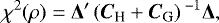 (2)
(2)
where Δ is the 5 × 1 matrix of the parameter differences, CH, CG are the covariance matrices for the corresponding parameters in the HIPPARCOS catalogue and the (propagated) Gaia data, and Δ′ is the transpose of Δ. Confidence intervals of the estimated ρ were obtained from the increase in χ2(ρ) around the minimum value; in particular, the 68% confidence interval (± 1σρ) is where 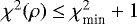 (Press et al. 2007). For the HIPPARCOS data, we used the re-reduction by van Leeuwen (2007), with covariances computed as described in Appendix B of Michalik et al. (2014).
To identify HIPPARCOS stars in Gaia EDR3, we used the cross-match table gaiaedr3.hipparcos2_best_neighbour provided with the release; of the 99 525 HIPPARCOS entries in that table, 98 004 have valid positions and proper motions in both catalogues. However, it is not meaningful to attempt to estimate the radial velocity for all of them. As indicated by Eq. (1), the precision on ρ mainly depends on the size of the product μϖ, and we therefore consider only the 13 161 sources in this sample that have μϖ > 1000 mas2 yr−1 in EDR3.
The practical implementation of the method to estimate ρ is complicated by the need to use a very accurate algorithm for propagating the astrometric parameters and by possible systematic differences between the Gaia and HIPPARCOS data sets. We used the propagation formulae derived by Butkevich & Lindegren (2014), which assume uniform rectilinear motion relative to the SSB and rigorously take light-time effects into account in addition to the geometric effects in Eq. (1).
In Gaia EDR3, there are known issues with the parallax zero point as well as with the reference frame of the bright stars (G ≲ 13, which includes all HIPPARCOS stars). Moreover, the HIPPARCOS reference frame may differ systematically from the EDR3 frame even after the latter has been corrected for the known issues (e.g. Brandt 2021). All of this could produce errors of the order of 1 mas and 0.2 mas yr−1 in the calculated parameter differences Δ in Eq. (2), which would affect our estimation of ρ. In order to minimise their impact, we used the following correction procedure in three steps. In the first step, the EDR3 data were corrected by subtracting the parallax bias according to Lindegren et al. (2021) and the magnitude-dependent proper motion bias according to Cantat-Gaudin & Brandt (2021). The resulting EDR3 data are, to the best of our knowledge, absolute and on a non-rotating reference frame for all magnitudes.
In the second step, we propagated the corrected EDR3 data to the HIPPARCOS epoch and analysed the HIPPARCOS–Gaia differences in position and proper motion in terms of an orientation error (ε) and spin (ω) of the HIPPARCOS reference frame with respect to the (corrected) Gaia frame. This used the equations
![Mathematical equation: \begin{equation*}\begin{bmatrix} (\alpha_{\textrm{H}}-\alpha_{\textrm{G}})\cos\delta \\[6pt] \delta_{\textrm{H}}-\delta_{\textrm{G}} \end{bmatrix} = \vec{M}\vec{\varepsilon}, \quad\quad \begin{bmatrix} \mu_{\alpha*,\textrm{H}}-\mu_{\alpha*,\textrm{G}} \\[6pt]\mu_{\delta,\textrm{H}}-\mu_{\delta,\textrm{G}} \end{bmatrix} = \vec{M}\vec{\omega},\end{equation*}](/articles/aa/full_html/2021/08/aa41344-21/aa41344-21-eq5.png) (3)
(3)
where the subscript H refers to the HIPPARCOS data as published by van Leeuwen (2007), G refers to the corrected and propagated Gaia data, and
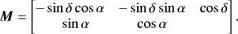 (4)
(4)
Using least-squares solutions weighted by the inverse combined variances, as in Eq. (2), this resulted in the estimates
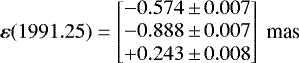 (5)
(5)
and
 (6)
(6)
Initially thefull set of 98 004 sources was included; however, after iteratively removing sources with significant residuals (mainly binaries), the final solutions used 86 914 sources for ε and 96 400 sources for ω. The uncertainties were estimated by bootstrap resampling. The offsets in Eqs. (5) and (6) are consistent with the estimated uncertainties of the HIPPARCOS reference frame, namely ± 0.6 mas for the components of ε(1991.25) and ± 0.25 mas yr−1 for the components of ω (Kovalevsky et al. 1997).
In the third and final step, the HIPPARCOS data were transformed to the (corrected) Gaia reference frame by subtracting Mε from the positions and Mω from the proper motions. These were then used together with corrected Gaia data to compute the parameter differences Δ in Eq. (2).
The various systematic corrections to the parallaxes and, in particular, the proper motions have a small but not entirely negligible impact on the estimated values of ρ. However, if none of the above corrections were applied, the resulting changes in ρ would in most cases be less than ±0.3σρ.
We note that other researchers have used similar techniques of combining HIPPARCOS and Gaia data for the somewhat orthogonal purpose of identifying astrometric binaries and stars dynamically accelerated by faint companions. Investigations based on the second release (DR2) of Gaia data include Brandt (2018) and Kervella et al. (2019), while Brandt (2021) provides an update using EDR3. In these studies the perspective effect was removed by adopting the spectroscopic radial velocity, when available, for the radial motion. In principle, the resulting χ2 (or similar) then includes a contribution from a possible difference between the astrometric and spectroscopic velocities; however, in general our method tends to give a high  for the same stars that are identified as accelerated in these other studies.
4 Determined radial velocities
When the algorithm outlined above is applied to the selected sample of HIPPARCOS stars, most of them obtain physically unrealistic values of ρ and/or very large formal uncertainties σρ. For 930 stars, we find | ρ | < 2000 km s−1 and σρ < 100 km s−1 and in Table 1 we give the results for the 55 entries among them having σρ < 10 km s−1. Of the 930 stars, all but four have spectroscopic radial velocities (vr) in the SIMBAD database (Wenger et al. 2000), and in Fig. 1 we show the distribution of ρ − vr for these stars as the light-blue histogram. Their median ρ − vr is + 2.3 km s−1 and the interquartile range (IQR) is 101.3 km s−1. The sub-sample of 852 stars that also have a reasonably good fit is shown in darker blue,  , indicating that the stars are perhaps not strongly perturbed by a companion. For these stars the median difference is + 1.2 km s−1 and the IQR is 95.5 km s−1.
For a number of the high-precision stars with small or moderate  , the agreement between the astrometric and spectroscopic values is remarkable. This is illustrated in the top panel of Fig. 2, where the two quantities are plotted against each other for the sub-sample with
  . The correlation is especially clear for the high-precision points shown in darker colours. Excluding the outlier van Maanen 2 (see Sect. 5.1), a least-squares fit to the remaining 851 data points, weighted by
  , yields
 (7)
(7)
The reduced chi-square of this fit is high, about 8.3, as can be expected from the presence of a number of binaries in the sample. The closeness of Eq. (7) to the equality relation ρ = vr, nevertheless, suggests that the binaries do not bias the population mean of ρ. The lower panel in Fig. 2 shows the velocity differences, with error bars, for the sub-sample in Table 1.
The uncertainties of ρ given in the table and diagrams are formal ones obtained as described in Sect. 3, based on the astrometric uncertainties provided in the HIPPARCOS and Gaia EDR3 catalogues. From a comparison of these two catalogues, Brandt (2021) concludes that the uncertainties in EDR3, for these bright sources, are underestimated by a factor of 1.37. If this is also the case for the present high-precision sub-sample, the uncertainties in Table 1 on average should be multiplied by a factor ≃ 1.2, and  by a factor ≃ 0.9. It would however have a negligible impact on the estimated values of ρ.
Many entries in Table 1 show a large discrepancy between ρ and vr (by many times the formal uncertainty)combined with a large  . These may be components of physical systems where the mutual perturbations cause dynamical accelerations that strongly bias the estimated ρ. A prime example is the binary system 61 Cyg AB (HIP 104214+104127), where the application of the method in Sect. 3 to the individual components gives
  of 249 and 29 285, respectively.
For binaries such as this, the method should instead be applied to the centre of mass (CM) of the system, yielding an estimate of the systemic ρ. Given the mass ratio q = MB∕MA, the astrometric parameters (a) of the CM in each catalogue can be computed as (aA + qaB)∕(1 + q), with covariance  . Propagatingthese parameters from EDR3 to the HIPPARCOS epoch and applying Eq. (2) yields a function χ2 (ρ, q) from which it may be possible to estimate both the (systemic) ρ and the mass ratio q.
Because the mass ratio equals the inverse ratio of the dynamical accelerations (e.g. Eq. (24) in Kervella et al. 2019), it is only possible to determine the mass ratio when the measured accelerations are significantlydifferent for the two components, leading to significantly different (and biased) estimates of ρ when the dynamical contributions are neglected. In addition to 61 Cyg AB (with Δρ ≡ ρB − ρA = −33.54 ± 3.76 km s−1), there are two other systems that fulfil this condition: HIP 91768+91772 (Δρ= −347.55 ± 9.80 km s−1) and HIP 45343+120005 (Δρ= −552.68 ± 41.26 km s−1). Estimates ofq and the centre-of-mass ρ for these systems are given in Table 2. For comparison, the table also gives the estimated ρ and  when the mass ratio is constrained to the value based on evolutionary models (for 61 Cyg, from Kervella et al. 2008), or the absolute K band magnitude (for GJ 338 and GJ725, from Kervella et al. 2019 using the calibration by Mann et al. 2015). The q values used in the constrained solutions are given without error limits in the second line of each object in Table 2. For a separate discussion of 61 Cyg AB, see Sect. 5.4.
For many more pairs, it is possible to compute a systemic ρ by assuming a particular value of q for the pair, for example, based on infrared photometry. While these estimates are less biased by dynamical acceleration than the component values ρA and ρB and, therefore, often in much better agreement with the spectroscopic values, we do not report them here as they are to a good approximation given by the weighted averages ρCM = (ρA + qρB)∕(1 + q).
5 Notes on individual objects
5.1 HIP 3829 (van Maanen 2)
In Fig. 2, one strikingly deviating point at vr = 263 km s−1 and ρ = −12 ± 7 km s−1 is van Maanen 2 (HIP 3829 or Wolf 28). At a distance of 4.3 pc, this is the closest single white dwarf and, after Sirius B and Procyon B, the third nearest. Theestimated ρ gives almost perfect agreement between the EDR3 and HIPPARCOS data ( for 4 dof).
Although the presence of a possible companion has been suggested, deep infrared imaging (Burleigh et al. 2008) and searches for binarity from possible proper-motion anomalies by Kervella et al. (2019) seem to exclude any nearby orbiting companion more massive than 2 MJup.
The strongly deviant spectroscopic value cannot be reconciled with the astrometric data for any reasonable amount of gravitational redshift. The spectroscopic number is the one generally quoted in catalogue compilations, entering databases such as SIMBAD (Duflot et al. 1995; Gontcharov 2006), and it merits closer scrutiny. In tracing the origins of this quantity, one finds it to come from the General Catalogue of Stellar Radial Velocities (Wilson 1953). Examining the remarks in the printed version of this catalogue2, one finds this value to arise from an observation made at Mt. Wilson Observatory, in a listing of stars with large radial velocities by Adams & Joy (1926). In that work, data for most stars are based upon several spectrograms, although ‘in a few cases of exceptional interest’, even a single observation was included. The stars are typically of visual magnitude 7–9, with van Maanen 2 being the faintest of that sample at V = 12.3 (the second faintest had V = 10.8). Only one exposure was recorded with the lowest resolution camera, and the deduced value is further marked as ‘subject to especial uncertainty’. Clearly, this cannot be seen as a precise or reliable measurement.
Together with other white dwarfs, van Maanen 2 was later observed with the Hale telescope on Palomar by Greenstein & Trimble (1967), yielding vr = +54 km s−1, a value those authors classified as ‘reliable’. In a somewhat later reexamination, Greenstein (1972) arrived at + 39 km s−1 from measuring numerous spectrograms, but with differences between various spectral lines. For such faint sources with very diffuse spectral lines, measured values may fluctuate greatly depending on the spectrograph dispersion and the depth of photographic exposure (Greenstein 1954). Even more precise spectral recordings face challenges: by using only the Ca II K line, Aannestad et al. (1993) obtained vr = +15 km s−1, but a fit to both the H and K lines instead gave + 54 km s−1, probably influenced by pressure shifts in the white-dwarf atmosphere.
The large proper motion of van Maanen 2 caused Oort (1932, page 287), expanding on an earlier suggestion by Russell & Atkinson (1931), to suggest the use of secular changes in proper motion to distinguish the gravitational redshift from actual radial motion, envisioned to be feasible after 30 or 40 yr of observations. Using the long-focus Sproul refractor during 1937–1970, van de Kamp (1971) derived a value for the astrometric velocity, with a significant uncertainty but remarkably consistent with the early spectroscopic measurements. However, Gatewood & Russell (1974) pointed out an error in those calculations. Using images from even longer time series with the Allegheny refractor, they deduced a new value with an astrometric velocity of + 6 ± 15 km s−1 and argued that this implies a plausible gravitational redshift. The Sproul plate series were continued until 1976, and they were re-measured by Hershey (1978), who then found an astrometric value of + 25 ± 18 km s−1.
The actual gravitational redshift depends on the white-dwarf mass. In a spectrophotometric study, Giammichele et al. (2012) obtained the mass 0.68±0.02 M⊙, implying a likely redshift of the order of 40 km s−1, thus leaving a contribution to the wavelength shift caused by the stellar motion that is reasonably consistent with our astrometric value of − 12 ± 7 km s−1.
The misperception of the anomalously large spectroscopic value for this star seems to have originated by the quoting and re-quoting of one particular uncertain observation, whereupon its inclusion in general catalogues was chosen as being the value that had the greatest number of citations. Such a case is by no means unique. For an example where early 19th century visual observations of suggested stellar variability were carried over into modern catalogues, see Dravins et al. (1993).
Estimated astrometric radial velocities for selected HIPPARCOS stars in order of increasing formal uncertainty.
Estimated systemic astrometric radial velocities and mass ratios for physical pairs.
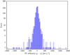 |
Fig. 1 Distribution of the difference ρ − vr between the astrometric and spectroscopic radial velocities for two samples of HIPPARCOS stars. Light blue: 926 stars with | ρ | < 2000 km s−1, σρ < 100 km s−1, and with radial velocities in SIMBAD. Dark blue: sub-sample of 852 stars that, in addition, have
|

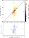 |
Fig. 2 Comparison of the astrometric and spectroscopic radial velocities. Top: astrometric versus spectroscopic values for the sample shown as the dark blue histogram in Fig. 1 and colour-coded according to the formal uncertainty (σρ) of the astrometric radial velocity estimate. The black line is the 1:1 relation. There are 28 data points that fall outside the limits ofthis plot. Bottom: difference between the astrometric and spectroscopic velocities for the sub-sample with σρ < 10 km s−1 (corresponding to Table 1), with error bars at ±σρ. There are 11 data points outside of this plot. |
5.2 HIP 57367 (LAWD 37)
Obtaining accurate gravitational redshifts in white dwarfs remains a challenge. Only in the particular nearby system of Sirius B, observed from Hubble Space Telescope, has a precise value of 80.65 ± 0.77 km s−1 been measured for its rather massive white dwarf (Barstow et al. 2005; Joyce et al. 2018).
In Table 1 the white dwarf with the most precise determination of astrometric radial velocity is LAWD 37 (HIP 57367 or GJ 440) with ρ = +28 ± 5 km s−1. As van Maanen 2, it fits the combined HIPPARCOS and Gaia EDR3 astrometry almost perfectly and has no known companion (Schroeder et al. 2000; Kervella et al. 2019). It does not have a spectroscopic velocity in SIMBAD, but it is clearly an interesting target for the determination of the gravitational redshift if a spectroscopic vr is obtained and an improved astrometric value can be derived using future releases of Gaia data. The significance of such data is enhanced by the prospects of measuring its mass from gravitational microlensing (Klüter et al. 2020; McGill et al. 2018, 2020).
Based on HIPPARCOS and Gaia DR2 data, Kervella et al. (2019) identified a proper-motion anomaly for LAWD 37 at a signal-to-noise ratio of 4.9, which could suggest the presence of a massive companion. That result, however, is not supported by the present study.
5.3 HIP 87937 (Barnard’s star)
This nearby red dwarf yields the most precise velocity value, with an uncertainty comparable to the star’s expected gravitational redshift. At these accuracy levels, differences between spectroscopic and astrometric values may start to provide unique astrophysical information. A feature of both Barnard’s star and other red dwarfs, is the presence of additional effects that are modulating the stellar spectrum. Precise Doppler monitoring sets limits on possible exoplanets (Choi et al. 2013; Kürster et al. 2003; Zechmeister et al. 2009), while variability in chromospheric emission lines suggests a long-term activity cycle (Gomes da Silva et al. 2012; Toledo-Padrón et al. 2019), accompanied by occasional flaring (Paulson et al. 2006). ‘Chromatic’ radial velocities obtained from different parts of the spectrum may segregate signatures from magnetic activity, convection, or other effects (Baroch et al. 2020); however, obtaining a zero point for the different wavelength shifts, corresponding to the radial motion of the stellar centre-of-mass, does require astrometry.
Analogous considerations apply to other red dwarfs including Proxima Centauri and Kapteyn’s star. Nearby red dwarfs are numerous (making up 35 out of the 55 entries in Table 1), and they can be expected to display statistically similar properties. Even if an adequate accuracy cannot yet be obtained for each of them, there is the prospect of averaging astrometric and spectroscopic velocities for groups of such M-dwarfs to identify features in their spectroscopic signatures once adequate data are available for a sufficient number of them. As mentioned in connection with Eq. (7), the possible presence of perturbing companions to some of the stars should not systematically bias the mean astrometric radial velocity for such a group.
5.4 HIP 104214 + 104217 (61 Cyg AB)
For the binary system 61 Cyg AB, we derived the mass ratio MB ∕MA = 0.758 ± 0.049 from the combined HIPPARCOS and Gaia EDR3 astrometry. This gives a significantly better fit to the combined astrometry than the higher mass ratio 0.877 estimated from evolutionary models by Kervella et al. (2008). As discussed therein, the masses of the components are not well constrained by observations and the mass ratio derived here is well within the range of previous dynamical estimates. However, both components are very bright for Gaia (G = 4.77 and 5.45 mag) and the astrometry in EDR3 is known to degrade rapidly for G ≲ 6 mag (Lindegren et al. 2018), which could bias our result.
In Dravins et al. (1999), we derived an astrometric radial velocity for 61 Cyg of ρ = −68.0 ± 11.1 km s−1. This was obtained from a combination of HIPPARCOS data and the visual observations by Bessel (1838), made in 1837–38 as part of his successful campaign to measure the parallax of the system. Considering that the perspective effect in position increases quadratically with the temporal baseline, it might still be relevant to consider Bessel’s measurements in combination with the Gaia and HIPPARCOS data. However, we have not been able to obtain a consistent solution including all three kinds of data. If this inconsistency would be caused by the problem in EDR3 mentioned above for the very bright stars, the results in Table 2 for this system should be viewed with caution.
6 Conclusions
The feasibility of determining radial velocities from purely geometric measurements was already realised long ago, along with its ensuing observational demands. In evaluating the observability of van Maanen’s star, Russell & Atkinson (1931) wrote: ‘in a century or less the true radial velocity of a star of such large proper motion and parallax as this could be found from the second order term in the proper motion’. Accuracies realised in space astrometry now permit such measurements over more manageable timescales. The most precise results should be obtainable for the nearest stars but, unfortunately, the brighter of those are still difficult to observe. Proxima Centauri yielded a precise value (Table 1), but the other components of the α Cen system weretoo bright to be included in Gaia EDR3 and they may have to be tied to the Gaia reference frame by means of other instruments (e.g. Akeson et al. 2021) or await future exploration of space observations. Already now, the method permits one to estimate gravitational redshifts of white dwarfs and to set limits on convective shifts in other stars.
Acknowledgements
This work has made use of data from the European Space Agency (ESA) mission Gaia (https://www.cosmos.esa.int/gaia), processed by the Gaia Data Processing and Analysis Consortium (DPAC, https://www.cosmos.esa.int/web/gaia/dpac/consortium). Funding for the DPAC has been provided by national institutions, in particular the institutions participating in the Gaia Multilateral Agreement. The work by LL is supported by the Swedish National Space Agency. The work by DD is supported by grants from The Royal Physiographic Society of Lund. This research has made use of the SIMBAD database, operated at CDS, Strasbourg, France. Diagrams were produced using the astronomy-oriented data handling and visualisation software TOPCAT (Taylor 2005). Use was made of NASA’s ADS Bibliographic Services and the arXivⓇ distribution service. We thank the referee, Pierre Kervella, for his detailed and insightful comments.
References
- Aannestad, P. A., Kenyon, S. J., Hammond, G. L., & Sion, E. M. 1993, AJ, 105, 1033 [NASA ADS] [CrossRef] [Google Scholar]
- Adams, W. S., & Joy, A. H. 1926, PASP, 38, 121 [CrossRef] [Google Scholar]
- Akeson, R., Beichman, C., Kervella, P., Fomalont, E., & Benedict, G. F. 2021, AJ, 162, 14 [CrossRef] [Google Scholar]
- Baroch, D., Morales, J. C., Ribas, I., et al. 2020, A&A, 641, A69 [EDP Sciences] [Google Scholar]
- Barstow, M. A., Bond, H. E., Holberg, J. B., et al. 2005, MNRAS, 362, 1134 [CrossRef] [Google Scholar]
- Bessel, F. W. 1838, Astron. Nachr., 16, 65 [NASA ADS] [CrossRef] [Google Scholar]
- Brandt, T. D. 2018, ApJS, 239, 31 [NASA ADS] [CrossRef] [Google Scholar]
- Brandt, T. D. 2021, ApJS, 254, 42 [CrossRef] [Google Scholar]
- Burleigh, M. R., Clarke, F. J., Hogan, E., et al. 2008, MNRAS, 386, L5 [NASA ADS] [CrossRef] [Google Scholar]
- Butkevich, A. G., & Lindegren, L. 2014, A&A, 570, A62 [NASA ADS] [CrossRef] [EDP Sciences] [Google Scholar]
- Cantat-Gaudin, T., & Brandt, T. D. 2021, A&A, 649, A124 [CrossRef] [EDP Sciences] [Google Scholar]
- Choi, J., McCarthy, C., Marcy, G. W., et al. 2013, ApJ, 764, 131 [NASA ADS] [CrossRef] [Google Scholar]
- de Bruijne, J. H. J., Hoogerwerf, R., & de Zeeuw, P. T. 2001, A&A, 367, 111 [NASA ADS] [CrossRef] [EDP Sciences] [Google Scholar]
- Dravins, D., Lindegren, L., Nordlund, A., & Vandenberg, D. A. 1993, ApJ, 403, 385 [NASA ADS] [CrossRef] [Google Scholar]
- Dravins, D., Lindegren, L., & Madsen, S. 1999, A&A, 348, 1040 [NASA ADS] [Google Scholar]
- Duflot, M., Figon, P., & Meyssonnier, N. 1995, A&AS, 114, 269 [Google Scholar]
- Gaia Collaboration (Brown, A. G. A., et al.) 2021, A&A, 649, A1 [NASA ADS] [CrossRef] [EDP Sciences] [Google Scholar]
- Gatewood, G.,& Russell, J. 1974, AJ, 79, 815 [NASA ADS] [CrossRef] [Google Scholar]
- Giammichele, N., Bergeron, P., & Dufour, P. 2012, ApJS, 199, 29 [NASA ADS] [CrossRef] [Google Scholar]
- Gomes da Silva, J., Santos, N. C., Bonfils, X., et al. 2012, A&A, 541, A9 [NASA ADS] [CrossRef] [EDP Sciences] [Google Scholar]
- Gontcharov, G. A. 2006, Astron. Lett., 32, 759 [NASA ADS] [CrossRef] [Google Scholar]
- Greenstein, J. L. 1954, AJ, 59, 322 [CrossRef] [Google Scholar]
- Greenstein, J. L. 1972, ApJ, 173, 377 [CrossRef] [Google Scholar]
- Greenstein, J. L., & Trimble, V. L. 1967, ApJ, 149, 283 [NASA ADS] [CrossRef] [Google Scholar]
- Hershey, J. L. 1978, AJ, 83, 197 [CrossRef] [Google Scholar]
- Joyce, S. R. G., Barstow, M. A., Holberg, J. B., et al. 2018, MNRAS, 481, 2361 [NASA ADS] [CrossRef] [Google Scholar]
- Kervella, P., Mérand, A., Pichon, B., et al. 2008, A&A, 488, 667 [NASA ADS] [CrossRef] [EDP Sciences] [Google Scholar]
- Kervella, P., Arenou, F., Mignard, F., & Thévenin, F. 2019, A&A, 623, A72 [NASA ADS] [CrossRef] [EDP Sciences] [Google Scholar]
- Klüter, J., Bastian, U., & Wambsganss, J. 2020, A&A, 640, A83 [CrossRef] [EDP Sciences] [Google Scholar]
- Kovalevsky, J., Lindegren, L., Perryman, M. A. C., et al. 1997, A&A, 323, 620 [NASA ADS] [Google Scholar]
- Kürster, M., Endl, M., Rouesnel, F., et al. 2003, A&A, 403, 1077 [NASA ADS] [CrossRef] [EDP Sciences] [Google Scholar]
- Leão, I. C., Pasquini, L., Ludwig, H. G., & de Medeiros, J. R. 2019, MNRAS, 483, 5026 [NASA ADS] [CrossRef] [Google Scholar]
- Lindegren, L., & Dravins, D. 2003, A&A, 401, 1185 [NASA ADS] [CrossRef] [EDP Sciences] [Google Scholar]
- Lindegren, L., Madsen, S., & Dravins, D. 2000, A&A, 356, 1119 [NASA ADS] [Google Scholar]
- Lindegren, L., Hernández, J., Bombrun, A., et al. 2018, A&A, 616, A2 [NASA ADS] [CrossRef] [EDP Sciences] [Google Scholar]
- Lindegren, L., Bastian, U., Biermann, M., et al. 2021, A&A, 649, A4 [EDP Sciences] [Google Scholar]
- Madsen, S., Dravins, D., & Lindegren, L. 2002, A&A, 381, 446 [NASA ADS] [CrossRef] [EDP Sciences] [Google Scholar]
- Madsen, S., Dravins, D., Ludwig, H.-G., & Lindegren, L. 2003, A&A, 411, 581 [NASA ADS] [CrossRef] [EDP Sciences] [MathSciNet] [PubMed] [Google Scholar]
- Mann, A. W., Feiden, G. A., Gaidos, E., Boyajian, T., & von Braun, K. 2015, ApJ, 804, 64 [CrossRef] [Google Scholar]
- McGill, P., Smith, L. C., Evans, N. W., Belokurov, V., & Smart, R. L. 2018, MNRAS, 478, L29 [NASA ADS] [CrossRef] [Google Scholar]
- McGill, P., Everall, A., Boubert, D., & Smith, L. C. 2020, MNRAS, 498, L6 [CrossRef] [Google Scholar]
- Meunier, N. 2021, ArXiv e-prints, [arXiv:2104.06072] [Google Scholar]
- Michalik, D., Lindegren, L., Hobbs, D., & Lammers, U. 2014, A&A, 571, A85 [NASA ADS] [CrossRef] [EDP Sciences] [Google Scholar]
- Moschella, M., Slone, O., Dror, J. A., Cantiello, M., & Perets, H. B. 2021, ArXiv e-prints, [arXiv:2102.01079] [Google Scholar]
- Oort, J. H. 1932, Bull. Astron. Inst. Netherlands, 6, 249 [Google Scholar]
- Pasquini, L., Melo, C., Chavero, C., et al. 2011, A&A, 526, A127 [NASA ADS] [CrossRef] [EDP Sciences] [Google Scholar]
- Paulson, D. B., Allred, J. C., Anderson, R. B., et al. 2006, PASP, 118, 227 [Google Scholar]
- Perryman, M. A. C., Lindegren, L., Kovalevsky, J., et al. 1997, A&A, 500, 501 [NASA ADS] [Google Scholar]
- Pourbaix, D., Nidever, D., McCarthy, C., et al. 2002, A&A, 386, 280 [NASA ADS] [CrossRef] [EDP Sciences] [Google Scholar]
- Press, W., Teukolsky, S., Vetterling, W., & Flannery, B. 2007, Numerical Recipes: The Art of Scientific Computing, 3rd ed. (Cambridge University Press) [Google Scholar]
- Ristenpart, F. 1902, Vierteljahrsschrift Astron. Ges., 37, 242 [Google Scholar]
- Russell, H. N., & Atkinson, R. D. 1931, Nature, 127, 661 [CrossRef] [Google Scholar]
- Schlesinger, F. 1917, AJ, 30, 137 [NASA ADS] [CrossRef] [Google Scholar]
- Schroeder, D. J., Golimowski, D. A., Brukardt, R. A., et al. 2000, AJ, 119, 906 [NASA ADS] [CrossRef] [Google Scholar]
- Seeliger, H. 1900, Astronom. Nachr., 154, 65 [NASA ADS] [CrossRef] [Google Scholar]
- Taylor, M. B. 2005, ASP Conf. Ser., 347, 29 [Google Scholar]
- Toledo-Padrón, B., González Hernández, J. I., Rodríguez-López, C., et al. 2019, MNRAS, 488, 5145 [Google Scholar]
- van de Kamp, P. 1971, in White Dwarfs, IAU Symp., ed. W. J. Luyten, 42, 32 [CrossRef] [Google Scholar]
- van de Kamp, P. 1977, Vistas Astron., 21, 289 [NASA ADS] [CrossRef] [Google Scholar]
- van Leeuwen, F. 2007, Hipparcos, the New Reduction of the Raw Data, AASL, 350 (Springer) [Google Scholar]
- Wenger, M., Ochsenbein, F., Egret, D., et al. 2000, A&AS, 143, 9 [NASA ADS] [CrossRef] [EDP Sciences] [Google Scholar]
- Wilson, R. E. 1953, General Catalogue of Stellar Radial Velocities, Carnegie Institution of Washington Publ., 601, Washington DC, 344 [Google Scholar]
- Zechmeister, M., Kürster, M., & Endl, M. 2009, A&A, 505, 859 [NASA ADS] [CrossRef] [EDP Sciences] [Google Scholar]
With radial velocity expressed in km s−1 and the astrometric quantities in milliarcseconds (mas), mas per Julian year (yr), and mas yr−2, we have A = (149 597 870.7 km) × (648 000 000∕π mas rad −1)∕(365.25 × 86 400 s yr−1) = 9.7779222168… × 108 mas km yr s−1.
All Tables
Estimated astrometric radial velocities for selected HIPPARCOS stars in order of increasing formal uncertainty.
Estimated systemic astrometric radial velocities and mass ratios for physical pairs.
All Figures
|
Fig. 1 Distribution of the difference ρ − vr between the astrometric and spectroscopic radial velocities for two samples of HIPPARCOS stars. Light blue: 926 stars with | ρ | < 2000 km s−1, σρ < 100 km s−1, and with radial velocities in SIMBAD. Dark blue: sub-sample of 852 stars that, in addition, have
|
| In the text | |
|
Fig. 2 Comparison of the astrometric and spectroscopic radial velocities. Top: astrometric versus spectroscopic values for the sample shown as the dark blue histogram in Fig. 1 and colour-coded according to the formal uncertainty (σρ) of the astrometric radial velocity estimate. The black line is the 1:1 relation. There are 28 data points that fall outside the limits ofthis plot. Bottom: difference between the astrometric and spectroscopic velocities for the sub-sample with σρ < 10 km s−1 (corresponding to Table 1), with error bars at ±σρ. There are 11 data points outside of this plot. |
| In the text | |
Current usage metrics show cumulative count of Article Views (full-text article views including HTML views, PDF and ePub downloads, according to the available data) and Abstracts Views on Vision4Press platform.
Data correspond to usage on the plateform after 2015. The current usage metrics is available 48-96 hours after online publication and is updated daily on week days.
Initial download of the metrics may take a while.