| Issue |
A&A
Volume 652, August 2021
|
|
|---|---|---|
| Article Number | A81 | |
| Number of page(s) | 6 | |
| Section | Stellar structure and evolution | |
| DOI | https://doi.org/10.1051/0004-6361/202141052 | |
| Published online | 13 August 2021 | |
Hunt for extremely eccentric eclipsing binaries
1
Astronomical Institute, Charles University, Faculty of Mathematics and Physics, V Holešovičkách 2, 180 00 Praha 8, Czech Republic
e-mail: This email address is being protected from spambots. You need JavaScript enabled to view it.
2
Variable Star and Exoplanet Section of the Czech Astronomical Society, Vsetínská 941/78, 757 01 Valašské Meziříčí, Czech Republic
3
FZU – Institute of Physics of the Czech Academy of Sciences, Na Slovance 1999/2, 182 21 Praha, Czech Republic
Received:
12
April
2021
Accepted:
6
June
2021
Abstract
We report the very first analysis of 27 eclipsing binary systems with high eccentricities that sometimes reach up to 0.8. The orbital periods for these systems range from 1.4 to 37 days, and the median of the sample is 10.3 days. Star CzeV3392 (= UCAC4 623 022784), for example, currently is the eclipsing system with the highest eccentricity (e = 0.22) of stars with a period shorter than 1.5 days. We analysed the light curves of all 27 systems and obtained the physical parameters of both components, such as relative radii, inclinations, or relative luminosities. The most important parameters appear to be the derived periods and eccentricities. They allow constructing the period–eccentricity diagram. This eccentricity distribution is used to study the tidal circularisation theories. Many systems have detected third-light contributions, which means that the Kozai-Lidov cycles might also be responsible for the high eccentricities in some of the binaries.
Key words: binaries: eclipsing / stars: fundamental parameters
© ESO 2021
1. Introduction
Eclipsing binaries (hereafter EBs) still play a crucial role in astrophysics today (Southworth 2012), mainly because they are used as calibrators in stellar evolutionary models (Torres et al. 2010). However, another use of EBs is also widely found in the literature. In addition to their use as distance indicators, they can also serve as ideal sources for statistical studies of stellar populations, such as studies of period distributions in various stellar populations, mass ratio distributions, or period–eccentricity relations (see e.g., Tokovinin 2008).
Period–eccentricity relations are studied mainly because a certain limit of the maximum value of eccentricity for a particular period is expected. The circularisation is a very slow process, but it is also inevitable. It causes all eccentric orbits to be more circular. The efficiency of this effect strongly depends on the relative sizes of the stars, that is, their R/a ratios. This means that the systems that are close enough (compact systems) should be well circularised or are still very young. On the other hand, longer-period systems should still have some non-zero eccentricity. All of these were studied several times in the past (using different binary samples) as a consequence of the tidal interaction in these systems, see for example Sztakovics et al. (2019) or Mazeh (2008). For the eclipsing binaries, the Kepler satellite and the studies of eclipsing binaries detected in its fields were very important. Quite recently, a study (Benbakoura et al. 2021) analysed the red giants in eclipsing binaries and discussed the circularisation theories in these evolved stars. Another paper (Van Eylen et al. 2016) studied the sample of Kepler binaries with respect to their temperatures and found an agreement with the theory that hotter stars have longer circularisation times.
Therefore we decided to focus our attention on the still rather sparsely populated areas in the period–eccentricity diagram near the higher limit of eccentricity for the particular period. These new data can bring us some new limits for the maximum eccentricity and the tidal circularisation theories, or possibly for the study of Kozai-Lidov cycles. Such effect is able to excite the eccentricity to higher values, or even break up the whole system. A necessary condition is a third component in the system in addition to the inner eclipsing pair, however. A weak indication of such a putative third body should also be gained through an analysis of the light curves (hereafter LCs) when a conclusive level of third-light contribution is detected.
2. Current status of the topic
Only a rather limited number of papers on the P − e diagram for eclipsing binaries is published so far, with only a few attempts to identify these higher eccentric systems. For example the well-known catalogues of eccentric eclipsing binaries published in 2007 by Bulut & Demircan that were later updated by Kim et al. (2018) are surprisingly very incomplete in this aspect. The authors studied only the O − C diagrams and apsidal motions, but the light curve solutions published for some of the systems were not included, especially those with higher eccentricities. In particular, the apsidal motion and the orbital period are related (the rapid apsidal motion is usually present in shorter-period systems), therefore these systems with high eccentricities were missed because they are not so interesting for observers. Moreover, Kim et al. (2018) were a rather dubious source of information on eccentricity at times. For example, the system with the highest eccentricity in Kim et al. (2018) is V345 Lac with e = 0.54, but this information was later revised to a much lower value of 0.26 by Wolf et al. (2019). This is a quite typical situation when the method of the O − C diagram analysis alone is used to derive the eccentricity instead of a more reliable light curve analysis. The most eccentric system in Kim et al. (2018) therefore is the star V1143 Cyg (= HD 185912, see Lester et al. 2019) with a period of 7.64 days and an eccentricity of 0.538.
The P − e relation was studied several times for spectroscopic binaries (see e.g., Latham et al. 2002, or Meibom & Mathieu 2005) or other types of systems such as exoplanets (Jurić & Tremaine 2008). However, because it is relatively easy and straightforward to derive the eccentricity in case of eclipsing binaries, we decided to use these objects. The eclipsing systems were used to detect of higher eccenricities, for instance using the ASAS (Pojmanski & Maciejewski 2004) photometric surveys by Shivvers et al. (2014), which appears to be one of only a few dedicated studies focusing on the detection of high eccentricities. The authors found the highest eccentricity for system ASAS 144242−5904.1 with e = 0.64, which was the maximum eccentricity found for eclipsing binary at that time. The rather questionable eclipsing system IO Com with its eccentric orbit e = 0.69 and P = 53 d is still quite problematic because no secondary eclipse has been detected (Taş & Evren 2014). The rich and precise data provided by the Kepler satellite (Borucki et al. 2010) were analysed later and yielded a large number of detached and highly eccentric systems, one of which has an eccentricity of 0.845, but an orbital period of 265 d (Kjurkchieva et al. 2017). However, these highly eccentric systems usually have rather long orbital periods, and the most eccentric system with an orbital period shorter than 40 days has an eccentricity of 0.702. Unfortunately, these longer-period systems have only little effect on our study of the P − e diagram because the most interesting curvature lies in periods shorter than 50 days. This was the main motivation for our study.
3. Selected systems
We chose for our analysis binaries that satisfied the following criteria: (i) They were never studied before (to enlarge the sample of already known binaries with high eccentricities), (ii) they have good phase coverage of their light curves (only with well-covered LC are we able to derive the eccentricity conclusively enough), and (iii) their high eccentricities are obvious. The last point comes easily from the fact that with the publicly available databases today, we can identify systems with high eccentricities only when the photometric data are plotted with proper period. These most eccentric systems show two signs of their eccentric orbits. First, the displacement of the primary and secondary minima out of 0.0 and 0.5 phases, respectively. Second, the very different eclipse durations. A combination of these two approaches applies for most of the systems we present here.
All binaries presented and analysed below were found using one of these two methods. First, six systems were identified in the OGLE fields of the LMC galaxy. The whole set of 26 121 eclipsing binaries identified in the OGLE III dataset (Graczyk et al. 2011) was scanned and the most eccentric systems were chosen. Then we used OGLE III and OGLE IV data (Pawlak et al. 2016) for the subsequent analysis. A second part of our sample are the systems that were discovered by chance in the monitored fields of some already known system by the authors M.M. and Z.H. For these new binaries the new TESS photometry (Ricker et al. 2015) was downloaded and analysed. For obtaining the photometry from the raw TESS data, we used the tool lightkurve (Lightkurve Collaboration 2018). There was the usual problem with these TESS data that the pixels are too large and the photometry is sometimes contaminated with close components (which usually has nothing to do with the eclipsing binary itself). Sometimes the method of flattening these TESS fluxes provides rather problematic trends and artefacts. Therefore we have to be very cautious when comparing the TESS photometric data with other ground-based photometry, especially its eclipse depths. For these reasons, we plot the TESS photometry only relatively (i.e., the out-of-eclipse magnitude was set to 0.0). For only one system were we not able to obtain any TESS data, therefore we used for the LC analysis the other available photometry from ASAS (Pojmanski 2002), and ASAS-SN (Shappee et al. 2014, and Kochanek et al. 2017) databases.
For basic information about the selected stars, see Table 1. Their identification in various catalogues is presented. Here we would like to emphasize the steadily growing number of new eclipsing systems (more than 2200 at present) discovered and included in the Czech Variable Star Catalogue, CzeV (Skarka et al. 2017). Moreover, the position on the sky and magnitude out-of-eclipse is provided in the Table 1 together with some temperature or spectral information, if available.
Individual systems.
4. Analysis
For the whole analysis we used the software PHOEBE, ver 0.32svn (Prša & Zwitter 2005). It uses a classical Roche-based model by Wilson & Devinney (1971), with its later modifications. The eccentric orbit was also implemented. The only unknown issue therefore remains for the start of analysis: the period. However, the periodicity of these selected stars was easily detectable from the photometry. The TESS data provide a superb coverage and precision, while the OGLE database even provides a period directly for every detected eclipsing binary.
For the analysis we applied several simplifications. Due to missing spectroscopy and only very limited information about these stars, we applied the following assumptions: (i) the mass ratio was set to unity, (ii) the synchronicity parameters were also set to pseudo-synchronous rotation, and (iii) albedo and gravity brightening coefficients were set to their suggested values according to the particular temperature of the stars. The most problematic issue remains the effective temperature of the primary component, which has to be set and remain fixed during the whole fitting process. Because the spectroscopy is not available, the only piece of information we have are the photometric indices, which can be used for a rough estimate of the temperatures. For the stars in our Galaxy using the TESS data, we usually used the temperature estimate based on the Gaia DR2 data (Gaia Collaboration 2018), while for the stars in LMC using the OGLE data, we tried to estimate roughly the effective temperatures based on the dereddened photometric indices as published by Zaritsky et al. (2004) and Massey (2002). We are aware that our main goal is to derive the period and eccentricity, and not to derive the precise physical parameters of the components. Therefore these simplifications are probably not crucial.
We did not include any spots for modelling either. The only system showing some additional asymmetry is CzeV3304. Its LC cannot be properly modelled with eccentricity and reflection (albedo and gravity-brightening effects).
5. Results
All the results of the systems we analysed are plotted together in Fig. 1, where all the final fits are given together with the data. The widths of the eclipses are rather narrow at times, but it is important to plot the whole phase of the light curves, not only a part of it zoomed near the min-eclipses. Because very narrow eclipses cover only a small fraction of the whole period, the proper primary and secondary eclipses are sometimes covered with only a few data points. This is still adequate for a precise derivation of the eccentricity value for the particular system, however. The results of the fittings are given in Table 2 together with some basic parameters such as relative radii R/a and also the periods and eccentricities of all systems. The higher values of the eccentricities for the longer-period binaries is clearly visible. See the more detailed discussion of the P − e relation in the next section.
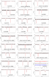 |
Fig. 1. Final light curves from our analysis. |
Parameters of the light-curve fits.
We plotted all light curves shifted in phase to always have the deeper minimum in 0.0, while the primary and secondary eclipses are also given in Table 2. These ephemerides for the primary and secondary should be used by future observers to plan their observations of both eclipses because the apsidal motion is negligible here. The hotter component is always the primary component, that is, the component with the derived fixed temperature from the values given in Table 1.
Although the individual masses are only roughly estimated and the mass ratio can only barely be derived for these detached systems (Terrell & Wilson 2005), our fits are thought to be reliable. They should be taken as good starting points for some future more detailed analyses of these systems, especially when good spectroscopy is available (then the need of a mass ratio fixed to unity would become obsolete). However, the missing mass ratio information can led to rather problematic results (e.g., the more luminous component is hotter, but smaller) that might also affect the resulting p–e values. The question is whether a problematic assumption in the beginning can lead to incorrect eccentricity values and if some significant offset of e can be caused by our method. To determine this, we tried the following test. A far more realistic LC solution (following the assumption of the main-sequence components) can be obtained using the method of mass ratio derivation by Graczyk (2003). This method uses the inferred luminosities of the two components to calculate the mass ratio, which is then more realistic. We used this method for the first two systems in our sample. For the first system, it resulted in exactly the same numbers as our simplified approach (as expected because the two components are very similar to each other). For the second system, UCAC4 750-003736, however, this more sophisticated approach led to q = 0.55 and e = 0.57. This eccentricity is even higher than the original (e = 0.54), even outside the original error bars. This means that the original uncertainties of the eccentricities are probably rather underestimated, a typical situation when using PHOEBE.
The detection of the third light (at a non-negligible level) for most of the systems was quite remarkable. About two-thirds of all binaries here appear to contain some additional component. This is a rather high fraction. Not all of them should be considered as triples in nature (because the quite large TESS pixels also cause close stars in the field to contribute to the signal, and a similar situation is known for the OGLE superdense LMC fields), but this result probably means that for a significant fraction of the stars, some triple-star dynamics cannot be completely excluded.
6. Discussion and conclusions
The discovery of several highly eccentric systems is still of great importance for the discussion of the period–eccentricity diagram (see Fig. 2) and tidal circularisation theories. The tendency of closer and more compact systems to orbit on more circular orbits was confirmed here. Moreover, some of the systems found here lie very close to the upper limit for the eccentricity for a particular period. These systems should be monitored in more detail in the next years as well. Zahn & Bouchet (1989) and their Fig. 1 or Khaliullin & Khaliullina (2011) and their Fig. 4 show that in serendipitous circumstances, when the eccentricity decrease is fastest, this eccentricity decline should be of about 0.001/100 yr. This lies just at the capability limits of current techniques. After some time (hundreds or thousands of orbits?), some circularisation should become visible in real time. This effect should be well observable in precise photometric data, which should later be compared to our solution. It also should be discussed whether some real change in eccentricity can be detected. The highly eccentric binaries should be most strongly affected.
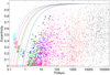 |
Fig. 2. Period–eccentricity diagram. Small black points are the data from the Orbit Catalog of Visual Binaries (Hartkopf et al. 2001), and small red points denote the spectroscopic binaries from the SB9 catalogue (Pourbaix et al. 2004). Green dots show eclipsing binaries from the catalogue of eccentric binaries by Kim et al. (2018), magenta dots show Kepler binaries by Kjurkchieva et al. (2017), and blue dots show those from ASAS published by Shivvers et al. (2014). The highly eccentric systems of this study are shown by the crosses. The colour curves represent the approximate limits of very close periastron approaches of the two components (i.e., 1.5 × R⋆ = a ⋅ (1 − e) and the semimajor axis a taken from Kepler’s third law) when they should collide with each other. The periastron distances were calculated for different spectral types (B to M) according to their typical radii and masses (Pecaut & Mamajek 2013), with the assumption that the two components are similar to each other (same masses and radii). |
The whole situation is clearly more complicated because tidal circularisation processes are differently effective for early- and late-type stars because of their internal structure (radiative and convective atmospheres). The two subsets of stars with a distinction between the different temperatures should therefore show a rather different P − e distribution. However, most of the data from Fig. 2 do not provide this information and thus cannot be easily divided into these two different groups of stars. The subset of SBs from Pourbaix et al. (2004) might preferentially contain the hotter stars, and in contrast, most of the EBs from Kepler (Kjurkchieva et al. 2017) are rather later spectral types, but it would be hard to clearly estimate the temperatures for the eccentric stars from Kim et al. (2018), or for the long-period visual binaries. Therefore we plot only our 27 systems in Fig. 3 in which these two subsets of hotter and cooler stars differ, and this is still a rather limited sample to show any difference between these two groups.
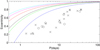 |
Fig. 3. Period–eccentricity diagram of our sample of stars with a distinction between the convective (circles) and radiative (crosses) stars according to the temperature estimates from Table 1. |
On the other hand, when we also take a possible role of the Kozai-Lidov cycles into account, the high eccentricity value detected here might be a consequence of the triple-star dynamics. The eccentricity of the inner pair can also be excited by the motion of the third star, and this effect can be much more rapid than the tidal circularization. Our high relative fraction of the detected systems with third light would slightly support this hypothesis. Only further investigation of this concern can confirm or refute any such hypothesis, not only with spectroscopy (convincingly detecting the third component), but also with good photometry obtained with much better angular resolution to separate the fluxes from the eclipsing pair itself and some possible close companion. The effect of a close companion that causes the photocenter shifts can also be studied using the precise TESS data (Sullivan et al. 2015), but that is beyond the scope of our analysis. To conclude, our study can be considered as a first step and calls for more detailed and dedicated observations, especially for these most eccentric targets in the close future.
Acknowledgments
At this place we would like to thank the referee of the manuscript, Dr. Andrei Tokovinin, whose helpful and critical suggestions greatly improved the quality of the manuscript. This research has made use of the SIMBAD and VIZIER databases, operated at CDS, Strasbourg, France and of NASA Astrophysics Data System Bibliographic Services. This research made use of Lightkurve, a Python package for TESS data analysis (Lightkurve Collaboration 2018). M.Mašek would like to thank to projects financed by Ministry of Education of the Czech Republic LM2018102 and LM2018105.
References
- Bai, Y., Liu, J., Bai, Z., et al. 2019, AJ, 158, 93 [CrossRef] [Google Scholar]
- Benbakoura, M., Gaulme, P., McKeever, J., et al. 2021, A&A, 648, A113 [CrossRef] [EDP Sciences] [Google Scholar]
- Borucki, W. J., Koch, D., Basri, G., et al. 2010, Science, 327, 977 [NASA ADS] [CrossRef] [PubMed] [Google Scholar]
- Bulut, I., & Demircan, O. 2007, MNRAS, 378, 179 [NASA ADS] [CrossRef] [Google Scholar]
- Gaia Collaboration (Brown, A. G. A., et al.) 2018, A&A, 616, A1 [NASA ADS] [CrossRef] [EDP Sciences] [Google Scholar]
- Graczyk, D. 2003, MNRAS, 342, 1334 [NASA ADS] [CrossRef] [Google Scholar]
- Graczyk, D., Soszyński, I., Poleski, R., et al. 2011, Acta Astron., 61, 103 [Google Scholar]
- Hartkopf, W. I., Mason, B. D., & Worley, C. E. 2001, AJ, 122, 3472 [NASA ADS] [CrossRef] [Google Scholar]
- Houk, N., & Smith-Moore, M. 1988, Michigan Catalogue of Two-dimensional Spectral Types for the HD Stars. Volume 4, Declinations–26°.0 to–12°.0. Department of Astronomy, University of Michigan, Ann Arbor, MI 48109–1090, USA. 14+505 pp. Price US 25.00 (USA, Canada), US 28.00 (Foreign) (1988) [Google Scholar]
- Jurić, M., & Tremaine, S. 2008, ApJ, 686, 603 [NASA ADS] [CrossRef] [Google Scholar]
- Khaliullin, K. F., & Khaliullina, A. I. 2011, MNRAS, 411, 2804 [CrossRef] [Google Scholar]
- Kim, C.-H., Kreiner, J. M., Zakrzewski, B., et al. 2018, ApJS, 235, 41 [NASA ADS] [CrossRef] [Google Scholar]
- Kjurkchieva, D., Vasileva, D., & Atanasova, T. 2017, AJ, 154, 105 [CrossRef] [Google Scholar]
- Kochanek, C. S., Shappee, B. J., Stanek, K. Z., et al. 2017, PASP, 129, 104502 [Google Scholar]
- Lasker, B. M., Lattanzi, M. G., McLean, B. J., et al. 2008, AJ, 136, 735 [NASA ADS] [CrossRef] [PubMed] [Google Scholar]
- Latham, D. W., Stefanik, R. P., Torres, G., et al. 2002, AJ, 124, 1144 [NASA ADS] [CrossRef] [Google Scholar]
- Lester, K. V., Gies, D. R., Schaefer, G. H., et al. 2019, AJ, 158, 218 [CrossRef] [Google Scholar]
- Lightkurve Collaboration (Cardoso, J. V. de M., et al.) 2018, Astrophysics Source Code Library [record ascl:1812.013] [Google Scholar]
- Liu, Z., Cui, W., Liu, C., et al. 2019, ApJS, 241, 32 [CrossRef] [Google Scholar]
- Massey, P. 2002, ApJS, 141, 81 [Google Scholar]
- Massey, P., Garmany, C. D., Silkey, M., et al. 1989, AJ, 97, 107 [NASA ADS] [CrossRef] [Google Scholar]
- Mazeh, T. 2008, EAS Publ. Ser., 29, 1 [CrossRef] [Google Scholar]
- Meibom, S., & Mathieu, R. D. 2005, ApJ, 620, 970 [NASA ADS] [CrossRef] [Google Scholar]
- Nassau, J. J., & Harris, D. 1952, ApJ, 115, 459 [CrossRef] [Google Scholar]
- Pawlak, M., Soszyński, I., Udalski, A., et al. 2016, Acta Astron., 66, 421 [Google Scholar]
- Pecaut, M. J., & Mamajek, E. E. 2013, ApJS, 208, 9 [Google Scholar]
- Pojmanski, G. 2002, AcA, 52, 397 [Google Scholar]
- Pojmanski, G., & Maciejewski, G. 2004, Acta Astron., 54, 153 [NASA ADS] [CrossRef] [Google Scholar]
- Pourbaix, D., Tokovinin, A. A., Batten, A. H., et al. 2004, A&A, 424, 727 [NASA ADS] [CrossRef] [EDP Sciences] [Google Scholar]
- Prša, A., & Zwitter, T. 2005, ApJ, 628, 426 [NASA ADS] [CrossRef] [Google Scholar]
- Ricker, G. R., Winn, J. N., Vanderspek, R., et al. 2015, J. Astron. Telescopes Instrum. Syst., 1, 014003 [Google Scholar]
- Shappee, B. J., Prieto, J. L., Grupe, D., et al. 2014, ApJ, 788, 48 [NASA ADS] [CrossRef] [Google Scholar]
- Shivvers, I., Bloom, J. S., & Richards, J. W. 2014, MNRAS, 441, 343 [CrossRef] [Google Scholar]
- Skarka, M., Mašek, M., Brát, L., et al. 2017, Open Eur. J. Variable Stars, 185, 1 [Google Scholar]
- Southworth, J. 2012, Orbital Couples: Pas de Deux in the Solar System and the Milky Way, 51 [Google Scholar]
- Sullivan, P. W., Winn, J. N., Berta-Thompson, Z. K., et al. 2015, ApJ, 809, 77 [NASA ADS] [CrossRef] [Google Scholar]
- Sztakovics, J., Forgács-Dajka, E., Borkovits, T., et al. 2019, EAS Publ. Ser., 82, 127 [CrossRef] [Google Scholar]
- Taş, G., & Evren, S. 2014, Baltic Astron., 23, 27 [Google Scholar]
- Terrell, D., & Wilson, R. E. 2005, Ap&SS, 296, 221 [NASA ADS] [CrossRef] [Google Scholar]
- Tokovinin, A. 2008, MNRAS, 389, 925 [NASA ADS] [CrossRef] [Google Scholar]
- Torres, G., Andersen, J., & Giménez, A. 2010, A&ARv, 18, 67 [Google Scholar]
- Van Eylen, V., Winn, J. N., & Albrecht, S. 2016, ApJ, 824, 15 [Google Scholar]
- Wilson, R. E., & Devinney, E. J. 1971, ApJ, 166, 605 [NASA ADS] [CrossRef] [Google Scholar]
- Wolf, M., Zasche, P., Kučáková, H., et al. 2019, Acta Astron., 69, 63 [Google Scholar]
- Zacharias, N., Finch, C. T., Girard, T. M., et al. 2013, AJ, 145, 44 [NASA ADS] [CrossRef] [EDP Sciences] [Google Scholar]
- Zahn, J.-P., & Bouchet, L. 1989, A&A, 223, 112 [Google Scholar]
- Zaritsky, D., Harris, J., Thompson, I. B., et al. 2004, AJ, 128, 1606 [NASA ADS] [CrossRef] [Google Scholar]
All Tables
All Figures
|
Fig. 1. Final light curves from our analysis. |
| In the text | |
|
Fig. 2. Period–eccentricity diagram. Small black points are the data from the Orbit Catalog of Visual Binaries (Hartkopf et al. 2001), and small red points denote the spectroscopic binaries from the SB9 catalogue (Pourbaix et al. 2004). Green dots show eclipsing binaries from the catalogue of eccentric binaries by Kim et al. (2018), magenta dots show Kepler binaries by Kjurkchieva et al. (2017), and blue dots show those from ASAS published by Shivvers et al. (2014). The highly eccentric systems of this study are shown by the crosses. The colour curves represent the approximate limits of very close periastron approaches of the two components (i.e., 1.5 × R⋆ = a ⋅ (1 − e) and the semimajor axis a taken from Kepler’s third law) when they should collide with each other. The periastron distances were calculated for different spectral types (B to M) according to their typical radii and masses (Pecaut & Mamajek 2013), with the assumption that the two components are similar to each other (same masses and radii). |
| In the text | |
|
Fig. 3. Period–eccentricity diagram of our sample of stars with a distinction between the convective (circles) and radiative (crosses) stars according to the temperature estimates from Table 1. |
| In the text | |
Current usage metrics show cumulative count of Article Views (full-text article views including HTML views, PDF and ePub downloads, according to the available data) and Abstracts Views on Vision4Press platform.
Data correspond to usage on the plateform after 2015. The current usage metrics is available 48-96 hours after online publication and is updated daily on week days.
Initial download of the metrics may take a while.