| Issue |
A&A
Volume 652, August 2021
|
|
|---|---|---|
| Article Number | A20 | |
| Number of page(s) | 12 | |
| Section | Astrophysical processes | |
| DOI | https://doi.org/10.1051/0004-6361/202141049 | |
| Published online | 03 August 2021 | |
Electron acceleration driven by the lower-hybrid-drift instability
An extended quasilinear model
1
Laboratoire Lagrange, Observatoire de la Côte d’Azur, Université Côte d’Azur, CNRS, Nice, France
e-mail: This email address is being protected from spambots. You need JavaScript enabled to view it.
2
Dipartimento di Fisica “E. Fermi”, Università di Pisa, Pisa, Italy
3
LPC2E, CNRS, Univ. d’Orléans, OSUC, CNES, Orléans, France
4
IRAP, CNRS-CNES-UPS, Toulouse, France
Received:
11
April
2021
Accepted:
13
May
2021
Abstract
Context. Density inhomogeneities are ubiquitous in space and astrophysical plasmas, particularly at contact boundaries between different media. They often correspond to regions that exhibit strong dynamics across a wide range of spatial and temporal scales. Indeed, density inhomogeneities are a source of free energy that can drive various instabilities such as the lower-hybrid-drift instability, which, in turn, transfers energy to the particles through wave-particle interactions and eventually heats the plasma.
Aims. Our study is aimed at quantifying the efficiency of the lower-hybrid-drift instability to accelerate or heat electrons parallel to the ambient magnetic field.
Methods. We combine two complementary methods: full-kinetic and quasilinear models.
Results. We report self-consistent evidence of electron acceleration driven by the development of the lower-hybrid-drift instability using 3D-3V full-kinetic numerical simulations. The efficiency of the observed acceleration cannot be explained by standard quasilinear theory. For this reason, we have developed an extended quasilinear model that is able to quantitatively predict the interaction between lower-hybrid fluctuations and electrons on long time scales, which is now in agreement with full-kinetic simulations results. Finally, we apply this new, extended quasilinear model to a specific inhomogeneous space plasma boundary, namely, the magnetopause of Mercury. Furthermore, we discuss our quantitative predictions of electron acceleration to support future BepiColombo observations.
Key words: plasmas / methods: numerical / instabilities / waves / methods: observational
© F. Lavorenti et al. 2021
 Open Access article, published by EDP Sciences, under the terms of the Creative Commons Attribution License (https://creativecommons.org/licenses/by/4.0), which permits unrestricted use, distribution, and reproduction in any medium, provided the original work is properly cited.
1. Introduction
Inhomogeneities in the magnetic field, velocity, density, temperature, etc. from fluid down to kinetic scales are commonly encountered in space and astrophysical plasmas (Amatucci 1999). The gradient associated with such inhomogeneous plasma regions is a source of “free” energy that can drive various kind of plasma instabilities. For instance, in the case of density gradient on scale close to the ion gyroradius, a situation that is commonly encountered in many plasma environments, the plasma is unstable against the so-called drift instabilities. These instabilities arise from the relative motion between ions and electrons, and turn out to be of paramount importance in shaping plasma boundaries found in space, allowing for strong anomalous mass and energy transport not achievable by standard collision-like diffusion.
In situ measurements show that lower-hybrid waves (LHW) with a frequency close to the lower-hybrid frequency  are ubiquitous in magnetized space plasma environments. Such waves are commonly observed at Earth’s magnetotail (Huba et al. 1978; Retinó et al. 2008; Zhou et al. 2009, 2014; Khotyaintsev et al. 2011; Norgren et al. 2012; Le Contel et al. 2017) and Earth’s magnetopause (André et al. 2001; Bale et al. 2002; Vaivads et al. 2004; Graham et al. 2017, 2019; Tang et al. 2020). In these two regions, LHW are commonly observed in the vicinity of magnetic reconnection sites where strong density gradients do form. Their role on the onset (or relaxation) of magnetic reconnection has been addressed in the past and still represents a key point in the context of reconnection research (Daughton 2003; Lapenta et al. 2003, 2018; Yoo et al. 2020).
Moreover, LHW are also observed at plasma shock fronts such as the terrestrial bow shock (Walker et al. 2008), interplanetary shocks in the solar wind (Krasnoselskikh et al. 1985; Zhang & Matsumoto 1998; Wilson et al. 2013), and supernova remnants (Laming 2001). Finally, LHW have been observed in induced ionosphere of comet 67P (André et al. 2017; Karlsson et al. 2017; Goldstein et al. 2019), of the planets Venus (Scarf et al. 1980; Shapiro et al. 1995) and Mars (Sagdeev et al. 1990), as well as at Earth’s ionosphere (Reiniusson et al. 2006). In this context, space observations of supra-thermal electron populations in conjunction with LHW represents one of the basic points motivating the interest in the study of the interaction of these waves with electrons (Norgren et al. 2012; Zhou et al. 2014; Le Contel et al. 2017; Broiles et al. 2016; Goldstein et al. 2019).
As more than just a mechanism at work in space plasma environments, electron acceleration by LHW is a mechanism commonly used in tokamak experiments to heat electrons and hence the plasma along the toroidal magnetic field lines (Bécoulet et al. 2011; Pericoli-Ridolfini et al. 1999). This naturally suggests that LHW generated in space are an efficient driver for electron acceleration in space plasma environments (Broiles et al. 2016). However, the mechanism for the generation of LHW in laboratory differs strongly from the one that is at play in space plasmas. In plasma fusion experiments, the LHW are commonly excited by an external pump enabling to sustain the waves and so the electron acceleration process on long time scales, with the parameters controlled by the experimenter himself. In inhomogeneous space plasma, LHW are instead generated by the development of plasma instabilities, in which nonlinear saturation might reduce the efficiency of the acceleration process when compared to plasma fusion experiments.
In a natural plasma environment, the two instabilities that can be responsible for the generation of LHW are: (i) the modified-two-stream instability (MTSI) driven by a supra-thermal ion beam (Ott et al. 1972; McBride et al. 1972; McBride & Ott 1972); and (ii) the lower-hybrid-drift instability (LHDI) driven by the relative drift between ions and electrons (Krall & Liewer 1971; Krall & Trivelpiece 1973; Gary 1993). The electron acceleration driven by LHW generated by the MTSI has been widely addressed in the literature using quasilinear theory (McBride et al. 1972; Shapiro et al. 1999), full-kinetic simulations (McClements et al. 1993; Bingham et al. 2002), and experiments (Rigby et al. 2018). The MTSI is considered the typical source for the above-mentioned LHW observations at plasma shock fronts (Krasnoselskikh et al. 1985; Shapiro et al. 1995, 1999) due to the reflection of a large fraction of solar wind ions by the shock front; however, LHW are routinely observed also in the absence of such beams of reflected ions, a condition that stands in the way of invoking the MTSI as the underlying mechanism. In such cases, the LHW are instead generated by the LHDI. The driver for the development of the LHDI has to be found in the “strong” density gradients that reach length scales on the order of, or even shorter than, the ion gyroradius. This is the case, for instance, for the above-mentioned observations at Earth’s magnetosphere and in cometary plasmas. Henceforth in this work, we focus on LHW generated by the LHDI and their interaction with the electron population.
The fastest growing modes of the LHDI propagate perpendicular to both the density gradient, say the x-direction, and the ambient magnetic field direction, the z-direction. The phase velocity is of the order of the ion thermal speed (Gary 1993). However, the LHDI modes are unstable over a narrow cone angle around this direction (in this case, the y-direction) proportional to the square root of the ion-to-electron mass ratio  (Gary & Sanderson 1978). This means that the oblique LHDI modes have a component of the phase velocity parallel (resp. perpendicular) to the ambient magnetic field of the order of the electron (resp. ion) thermal speed. As a result, electrons can be resonantly accelerated by LHDI fluctuations in the direction parallel to the ambient magnetic field through wave-particle interactions; hereafter, we refer to this mechanism as LHDI electron acceleration.
The goal of this paper is to investigate the efficiency of the LHDI electron acceleration. As of today, the state-of-the-art theoretical model of this mechanism is provided by the analytical quasilinear model proposed by Cairns & McMillan (2005), hereafter, called the QL model. The QL model is well suited to the study of the early stage of the electron acceleration, but eventually it breaks down when the nonlinear feedback from the particle distribution to the wave becomes important. More precisely, the QL model breaks down as soon as nonlinear effects locally modify the distribution function shape (i.e. around the resonant velocity); hereafter referred to as nonlinear LD-like effects because they are analogous to the well-known nonlinear Landau damping effects (see Brunetti et al. 2000 and references therein).
Other past works have addressed the problem of the interaction between pump-generated LHW and electrons, including such nonlinear LD-like effects (Singh et al. 1996, 1998; Zacharegkas et al. 2016). However, the configuration adopted in these works is not well suited for space plasma configurations where LHW are typically driven by a plasma instability, such as the LHDI, and not by an external pump. To the best of our knowledge, the LHDI electron acceleration mechanism has not yet been studied using a self-consistent full-kinetic model.
In the past, the efficiency of LHDI electron acceleration has been addressed by means of reduced analytical models similar to the QL model, mostly because of the limitations on computational resources. Indeed, the computational power required to solve the Vlasov equation for LHDI electron acceleration is challenging because (i) ion and electron kinetic physics must be included self-consistently in the model, meaning that a full-kinetic numerical simulation is required; and (ii) the wave propagation occurs over an angle, in the y − z plane, perpendicular to the inhomogenity direction, the x-direction, meaning that three-dimensional (3D) numerical simulations are required. All in all, investigating the electron acceleration generated by the LHDI requires full-kinetic 3D-3V simulations. This is one of the methods used in this work.
In this paper we investigate the electron acceleration associated with the LHDI through a comparison of complementary numerical simulations. We use the quasilinear approach and direct full-kinetic 3D-3V simulations. This enables us to assess the intrinsic limits of the QL model and to investigate the consequences of nonlinear LD-like effects on the LHDI electron acceleration. We present the first direct numerical evidence of LHDI electron acceleration from full-kinetic 3D-3V simulations, and we build up an extended quasilinear (eQL) model that takes into account the effect of such nonlinear saturation to quantitatively estimate electron acceleration under realistic space plasma parameters.
The paper is organized as follows: Section 2 describes the QL model and the full-kinetic 3D-3V simulation model we use here. Section 3 presents the results of both models using two common sets of plasma parameters (“strong” and “weak” gradient configurations). Section 4 compares the results of the two models, shows the limitations of the QL model as compared to the full-kinetic one, and presents a novel eQL model. Finally, we apply this new eQL model to the magnetopause of Mercury in view of the future observations of the BepiColombo space mission. Section 5 summarizes our findings and presents our conclusions.
2. Models and methods
In this study, we use two different models of plasma evolution. First, a QL model of LHDI electron interaction based on the work of Cairns & McMillan (2005). Second, a full-kinetic 3D-3V plasma simulations of a plasma boundary initially unstable to the LHDI. The former is a simplified model of the plasma dynamics that does not account for the full response of the plasma itself to nonlinear interactions, and is therefore considered a reduced model. The latter instead is fully self-consistent, even if constrained by a specific parameter choice, and it is therefore considered an ab initio model. The full-kinetic model, being more general than the QL one, is used to assess the limits of the latter and eventually, to build an extended description that properly models the LHDI electron acceleration still within a quasilinear framework.
2.1. Quasilinear analytical model
The wave-particle interaction between LHW (generated from LHDI) and electrons can be modeled using a powerful analytical tool: quasilinear theory (Bernstein & Engelmann 1966; Alexandrov et al. 1984). Quasilinear theory is based on a second order perturbative expansion of the Vlasov equation averaged over the spatial variables. The system of quasilinear equations describes: (i) the diffusion in velocity space of the electron distribution function through a diffusion coefficient proportional to the electric field energy (Eqs. (1) and (2)); and (ii) the time evolution of the electric field energy (Eqs. (3) and (4)). The state-of-the-art QL model for LHDI electron interaction is the one developed in Cairns & McMillan (2005) and summarized here:
 (1)
(1)
 (2)
(2)
![Mathematical equation: $$ \begin{aligned}&\partial _t S_k(k_{\bot },k_{\parallel },t) = \left[ \gamma _{\mathrm{LHDI}} \left( 1-\frac{S_k}{S_{k,\max }} \right) +\gamma _e(k_{\bot },k_{\parallel },t) \right] S_k, \end{aligned} $$](/articles/aa/full_html/2021/08/aa41049-21/aa41049-21-eq5.gif) (3)
(3)
 (4)
(4)
Here, fe(v∥, t) is the electron distribution function, k⊥ (resp. k∥) is the wavevector perpendicular (resp. parallel) to the ambient magnetic field,  is the electric field energy density in wavevector-space, Sk, max is the maximum value of Sk attained at saturation, n0 is the plasma density, ωLH, ωci are the lower-hybrid and ion cyclotron frequencies, ω(k⊥, k∥) is the spectrum of the wave, γLHDI is twice the linear growth rate of the LHDI, and δ(x) is the Dirac delta function. In the following, ρi is the ion gyroradius, and vthi = ρiωci is the ion thermal speed.
After normalization, this nonlinear system of coupled partial differential equations (Eqs. (1)–(4)) is solved by numerical integration using a time staggered leapfrog scheme. In k-space, we limit the computation to the region of LHDI fastest growing modes, that is, 0.7 < k⊥ρe < 1 and 0 < k∥ρi < 1, as done in Cairns & McMillan (2005). Since the wavevectors are limited to this region, the wave spectrum turns out to be more or less flat with a corresponding frequency for the fastest growing mode given by the lower-hybrid frequency, ω(k⊥, k∥) ≃ ωLH. The grid in velocity space is chosen by testing the convergence of the solution.
The QL model, Eqs. (1)–(4), depends on four parameters: mi/me, ωpe/ωce, γLHDI, and Sk, max. The first two parameters, mi/me, ωpe/ωce, define the plasma itself. The last two parameters γLHDI and Sk, max (or analogously Smax = ∫d3kSk, max) define the linear growth and saturation level of the instability, and they only depend on the initial plasma configuration. The analytical expressions for these two quantities are given by:
 (5)
(5)
 (6)
(6)
where βi is the ion plasma beta, and the inverse gradient scale length ϵn is defined as
 (7)
(7)
The growth rate γLHDI in Eq. (5) has been obtained using a linearized kinetic model by Davidson et al. (1977). The electric energy at saturation Smax in Eq. (6) has been obtained using an analytic quasilinear approach by Davidson (1978), and it was later tested numerically by Brackbill et al. (1984) using 2D full-kinetic simulations. The LHDI can saturate through two different processes depending on the initial value of the density gradient: ion trapping (resp. current relaxation) for high (resp. low) values of the density gradient (Brackbill et al. 1984).
The derivation of Eqs. (5) and (6) is based on the assumption that the only source of drift in the plasma is the density gradient. Thus, all particle drifts, apart from the diamagnetic drift vDi, are considered negligible. As a consequence, vDi/vthi = ϵnρi. In the full-kinetic simulations, presented in the next section (Sect. 2.2), this assumption is essentially verified.
Quasilinear models are inherently limited because they do not include the nonlinear feedback from the modified plasma dispersion function on the electromagnetic fields. To overcome this limitation, we present in the next section (Sect. 2.2) a full-kinetic 3D-3V numerical plasma model.
2.2. Setup for full-kinetic 3D-3V simulations
The full-kinetic model of the plasma is based on a direct solution of the Vlasov-Maxwell system of equations using a Lagrangian PIC (particle-in-cell) approach.
To run the simulations of a plasma boundary unstable to the LHDI, we used the explicit, electromagnetic, relativistic, PIC code SMILEI (Derouillat et al. 2018). The ambient magnetic field is directed along the z-axis and the density gradient along the x-axis. In order to model both wave propagation (predominantly along the y-axis, perpendicular to both the magnetic field and the density gradient direction) and the electron wave-particle interaction (predominantly along the z-axis, parallel to the magnetic field), we considered a 3D numerical box. Compared to previous numerical investigations of the LHDI (Brackbill et al. 1984; Gary & Sgro 1990; Hoshino et al. 2001; Shinohara & Hoshino 1999; Lapenta & Brackbill 2002), which focused on the wave generation mechanism only through 2D-3V simulations in the equivalent of our (x, y) plane, we also include in this study the out-of-plane direction that hosts the electron acceleration resonant processes. An overview of the numerical setup is shown in Fig. 1, with the right panel showing the 3D numerical box used here and highlighting: (i) a slice of the ion density field in the (x, y) plane; and (ii) the plane (y, z) that is most unstable to the LHDI in yellow.
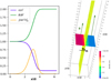 |
Fig. 1. Schematic view of the setup of the full-kinetic 3D-3V simulations presented in this study. Left panel: Density, magnetic field, and current profiles at t = 0 along the direction of the inhomogeneity (x-axis) in the “strong gradient” simulation. Right panel: 3D visualization of the ion density in the “strong gradient” simulation at |

The initialization of the simulations ensures pressure balance by means of the Vlasov equilibrium proposed in Alpers (1969), Pu et al. (1981), which shapes a plasma boundary with density and magnetic field asymmetries, uniform temperature, with no electric field and no velocity nor magnetic field shear. Hereafter, we refer to the side I (resp. side II) of this boundary as the high (resp. low) density side. The expressions for the initialization profiles are:
 (8)
(8)
 (9)
(9)
 (10)
(10)
Here, T = Ti + Te is the uniform temperature, PBC is the constant of pressure balance (set to have the plasma beta βI = 10/3 and βII = 1/12), and w is a constant that defines the width of the layer – set to 0.98 (resp. 0.5) in the “strong” (resp. “weak”) gradient case. We use a density and magnetic field asymmetry of nI/nII = 10 and BI/BII = 0.5. The shape of these initialization profiles is shown in the left panel of Fig. 1. In the following, all quantities are normalized to ion quantities in side I: the ion gyrofrequency,  ; the ion skin depth,
  ; and the Alfvén speed
  . The numerical box dimensions are: Lx = Ly = 2π and Lz = 20π, with a number of cells, namely, Nx = Ny = 288 and Nz = 1472. The box is elongated (by a factor of
  in the magnetic field direction in order to reliably include the narrow cone angle over which unstable LHDI modes grow. The timestep used in the simulations is dt = 3.4 × 10⁻⁴ to satisfy the CFL stability condition. The simulations are ran for several tens of the ion gyroperiods until electron acceleration saturates. We use 100 macro-particles per cell and a second order spline interpolation for the macro-particles. We use a reduced ion-to-electron mass ratio mi/me = 100 to make simulations computationally feasible while maintaining a sufficient scale separation between ions and electrons. The implications of using such a reduced mass ratio are discussed in Sect. 4. We use an ion-to-electron temperature ratio Ti/Te = 1, and a plasma-to-cyclotron frequency ratio of
  . The magnitude of the density asymmetry used in these simulations encompasses the typical parameters observed in small planetary magnetospheres such as Mercury (Gershman et al. 2015).
Two different simulations are investigated using two different layer widths: (i) a steeper boundary case (with the inverse gradient scale length ϵn = 1, defined in Eq. (7)), hereafter called a “strong gradient” simulation; and (ii) a smoother boundary case (with ϵn = 0.5), hereafter called the “weak gradient” simulation. These parameters are chosen to ensure that the amplitude of the LHDI fluctuations is well above the PIC noise level and also to saturate through the two different mechanisms introduced in Sect. 2.1: ion trapping or current relaxation.
3. Evolution of LHDI and associated electron acceleration: Simulations results
First, we show the results of the full-kinetic model. Then we show those obtained with the QL model using the same parameters as for the full-kinetic simulations. Finally, we compare the results of the two models showing the range of validity and the limitations of the QL model.
3.1. Results from the full-kinetic 3D-3V simulations
In both the “strong gradient” and “weak gradient” full-kinetic simulations, the layer is unstable to the LHDI due to the presence of a density gradient on ion kinetic scales. The LHDI fluctuations grow exponentially in the layer for times t < tsat as predicted by kinetic linear theory. The fastest growing mode (FGM) is electrostatic and directed along the y-axis with wavevector of kyρe ≈ 1, frequency of ω ⪅ ωLH and a growth rate of γ ⪅ ωLH, which are in agreement with the linear estimation (Eq. (5)) for both simulations. The growth of the electric field energy – normalized to the ion thermal energy and integrated over the unstable layer – is shown in Fig. 3 with green curves for both simulations. At t ≈ tsat (corresponding to the first vertical dashed lines in each panel of Fig. 3), the electric field fluctuation’s growth saturates. Using the growth rate and the saturation level from Eqs. (5) and (6), we compute the saturation time analytically as
![Mathematical equation: $$ \begin{aligned} t_{\rm sat}=\frac{\ln \left[ S_{\max }/S(t=0) \right] }{\gamma _{\mathrm{LHDI}}}. \end{aligned} $$](/articles/aa/full_html/2021/08/aa41049-21/aa41049-21-eq20.gif) (11)
(11)
We note that the initial amplitude of the electric field energy, S(t = 0) ≈ 10−4nTi in both simulations, is due to the particle noise intrinsic to the full-PIC algorithm that we use.
The saturation mechanism of the LHDI has been extensively addressed in the past, see, e.g., (Winske & Liewer 1978; Davidson 1978; Chen & Birdsall 1983; Brackbill et al. 1984), with results demonstrating that LHDI saturates because of ion trapping (resp. current relaxation) in the case of strong (resp. weak) density gradients. The saturation mechanisms at play in our simulations are shown in Fig. 2. First, in the strong gradient simulation, we give evidence for ion trapping (top left panel) in the potential well of the LH waves (bottom left panel). These phase space vortices are not observed in the weak gradient simulation. Second, we show a significantly stronger decrease of the total charge current in the layer in the weak gradient simulation (orange) compared to that in the strong gradient one (blue) (right panel). This is consistent with saturation taking place via current relaxation in the weak gradient simulation, that is, the LHDI fluctuations inhibit its source of free energy by reducing the electron drift in the layer. We conclude that in the strong gradient simulation the LHDI saturates due to ion trapping, while in the weak gradient simulation, the LHDI saturates due to current relaxation, as is expected based on past studies. This is further confirmed by the fact that in both cases, the saturation levels are comparable with the ones obtained by Eq. (6). Subsequently, in the strong gradient simulation, we observe for t > tsat a rapid decrease of the electric fluctuations amplitude, characteristic of an overshoot pattern, which is shown in the electric-to-thermal energy ratio in Fig. 3 (left panel, green curve) at a time t = tsat. Such an overshoot of the electric field fluctuations is not observed in the weak gradient simulation. An important point to note is that in both simulations, the electric field energy always remains much smaller than the thermal energy of the particles (it never exceeds 1%).
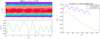 |
Fig. 2. Saturation mechanisms at play in the two simulations: ion trapping (left panels) and current relaxation (right panel). Left panels: isocontour of the ion phase space density (top panel) together with the electric potential of the LHDI waves (bottom panel) on the same spatial axis, both quantities being computed in the unstable layer. Right panel: evolution of the difference between the average charged current in the unstable layer (2 < x < 4) and its value at t = 0, for both simulations. |
We also note that a common issue with PIC simulations is the possible occurrence of spurious numerical heating of the macroparticles population during the simulation. This effect, due to the so-called “finite grid instability” (Birdsall & Langdon 1991; Markidis & Lapenta 2010; McMillan 2020), appears when the Debye length is not sufficiently resolved by the numerical grid. In such a case, the electrons would be numerically heated, which would hide the wave-particle interaction we are looking for. We carefully checked that our PIC simulations are free from such numerical spurious heating, by comparing the evolution of the supra-thermal electron density in the unstable layer to the one outside the layer on both sides, where the plasma is stable, to check that the numerical heating of the electrons is negligible compared to the one arising from wave-particle interaction in the layer.
To quantify the efficiency of the LHDI in accelerating electrons parallel to the ambient magnetic field, we define a supra-thermal electrons density as follows:
 (12)
(12)
Here, the supra-thermal electrons density Ne, sup is used as a quantitative tracer of the LHDI electron acceleration. The growth and saturation of Ne, sup is shown for both simulations in Fig. 3, with red curves.
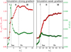 |
Fig. 3. Full-kinetic simulations: evolution of the electron supra-thermal density Ne, sup(t)/Ne, sup(0) (red curves) and of the electric field energy normalized to the ion thermal energy S/nTi(t) (green curves), both curves are integrated over the unstable layer (3.5 < x < 4 for strong gradient and 3.5 < x < 4.5 for weak gradient). We note that time axes are different for the two simulations. |
In both simulations, the efficiency of the LHDI electron acceleration process can be described through a three-phase evolution: (i) the linear phase, 0 < t < tsat; (ii) the quasilinear phase, tsat < t < τNL; and (iii) the strongly nonlinear phase, t > τNL. The characteristic time scales, tsat and τNL, computed from Eqs. (11) and (16), respectively, are marked in Fig. 3 by vertical dashed lines. The latter time scale constitutes the fundamental outcome of the full-kinetic model and an extensive discussion is provided in Sect. 4.2.
In the linear phase (phase I in Fig. 3), the electric field grows exponentially, as predicted by linear theory. In the weak gradient case, in phase I, the electron acceleration remains weak compared to the overall electron acceleration observed at saturation. This is understandable since the resonant electric field fluctuations themselves remain weak compared to their steady-state value at saturation. On the contrary, in the strong gradient case, in phase I, around tsat, the electric field of the LHDI waves reaches values even higher than the saturation value. As a result, we observe a non-negligible increase of the supra-thermal electron density in a very short time scale around tsat, this process is discussed in detail in Sect. 4.
In the quasilinear phase (phase II in Fig. 3), electron acceleration starts to take place as observed in both simulations. In this phase, the efficiency of the acceleration is directly related to the driver intensity (i.e., the stronger the electric field the stronger the acceleration), as expected from the QL diffusion equations (Eqs. (1) and (2)).
Finally, in the strongly nonlinear phase (phase III in Fig. 3), while the electric field amplitude remains constant and finite, the acceleration stops due to the onset of nonlinear LD-like effects.
Such a multi-phase evolution is observed in both strong and weak gradient simulations (see Fig. 3). One main difference between the two simulations is the presence – in the strong gradient simulation – of an overshoot in the electric energy, which is not observed in the weak gradient simulation. Such an overshoot corresponds to a sharp peak in the electric-to-thermal energy ratio at t ≈ tsat, which subsequently leads to a strong electron acceleration for the overshoot duration (see Fig. 3, left panel around tsat). However, the overall contribution of this phenomenon to the total amount of accelerated electrons is shown not to be significant in Sect. 4. In the end, for both simulations, the supra-thermal electron density in the inhomogeneous layer is increased by around 15%−20%. However, in the two cases, this same final value is attained through a different evolution: in the strong gradient simulation, the acceleration is faster but stops sooner (at τNL ≈ 10), while in the weak gradient simulation the acceleration occurs at a slower rate but remains efficient on longer time scales (up to τNL ≈ 40). Interestingly, these two effects seems to compensate each other.
The nonlinear LD-like time scale τNL, which is not accessible to quasilinear models, represents the original result of our full-kinetic simulations. An extensive discussion of this is given in Sect. 4.
3.2. Results of the standard quasilinear model
To enable a quantitative comparison between the QL model described in Sect. 2.1 and the full-kinetic one, the former is solved using the same plasma parameters as for the unstable layer of the full-kinetic simulations. More precisely, the input parameters of the QL model are obtained by averaging the plasma density, and the magnetic field in the layer 3.5 < x < 4 (resp. 3.5 < x < 4.5) for the strong (resp. weak) gradient full-kinetic simulation.
Numerical integration of the QL model (Eqs. (1)–(4)) provides the time evolution of the electron distribution function fe(vz) shown in Fig. 4 at different time instants. We observe a diffusion in velocity space for both “strong” and “weak” gradient cases, corresponding to electron acceleration by LHW. The characteristic timescale for such acceleration turns out to be of the order of hundreds of ion cyclotron periods. As expected, this time scale is longer in the weak gradient case than in the strong gradient one.
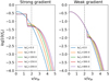 |
Fig. 4. Results of the QL model for the strong and weak gradient parameter case, shown in the left and right panel, respectively. Both panels show the electron distribution function at different time instants in the direction parallel to the magnetic field. Grey vertical dashed lines at v = 2vthe ≈ vphz correspond to the point from where the supra-thermal electron density (Eq. (12)) is computed. |
Eventually, electron acceleration described by QL theory slows down after long times. Indeed, as already explained in Cairns & McMillan (2005), the characteristic time scale to accelerate an electron of velocity v∥ by an amount δv∥ scales as  for δv∥ ∼ v∥. With the parameters used in our two simulations, the electron acceleration obtained from the QL model becomes negligible after time τDiff ⪆ 150 (resp. τDiff ⪆ 400) in the strong (resp. weak) gradient case, as shown in Fig. 4.
Such LHDI electron acceleration appears much weaker than those presented in the work of Cairns & McMillan (2005). This discrepancy is directly associated with the choice of the parameter Smax/nTi, the electric-to-thermal energy at the saturation of the LHDI, which is proportional to the quasilinear diffusion coefficient (Eq. (2)). In this study, we use Smax/nTi = 0.01 (resp. 0.002) for the strong (resp. weak) gradient case to obtain the results shown in Fig. 4. These values are obtained from Eq. (6) and are consistent with those observed in our full-kinetic simulations. Differently, in the seminal paper of Cairns & McMillan (2005) the authors have used a value Smax/nTi = 0.5 that is two orders of magnitude larger than what is expected from the theory of saturation of the LHDI in Davidson (1978) using the configuration considered in that study. Such a choice for an overestimated value of the parameter Smax/nTi unavoidably leads to an overestimation of the quasilinear diffusion coefficient and, therefore, of a higher electron acceleration efficiency. This indicates that a consistent choice of the electric-to-thermal energy ratio at saturation is crucial in quasilinear models in order to accurately assess a reliable value of the quasilinear diffusion coefficient.
Despite the different choice of the parameter Smax/nTi, the time evolution of the electron distribution function obtained with the QL model agrees qualitatively with the one presented in Cairns & McMillan (2005). The comparison with the evolution obtained from the full-kinetic model is given in the next section (Sect. 4.1).
4. Discussion: Toward an extended quasilinear model and beyond
In this section, we first compare the full-kinetic and standard quasilinear results, then we show the discrepancies between the two models, and we highlight the physical processes that give rise to such discrepancies. Next, in order to overcome the intrinsic limits of the standard quasilinear theory, we build an extended quasilinear model (eQL) that includes the consequences of nonlinear LD-like effects. Finally, we validate such eQL and extrapolate how it scales with the plasma parameters of interest (e.g., ion-to-electron mass ratio, gradient length) in order to enable its use beyond the two specific set of parameters of our full-kinetic simulations.
4.1. Comparison between the full-kinetic and the QL models
To quantitatively compare the results of the full-kinetic and QL models on LHDI electron acceleration, we focus on the evolution of the supra-thermal electron density (defined in Eq. (12)), shown for both strong and weak gradient cases in Fig. 5, where the two characteristic times, tsat and τNL, (previously identified from the full-kinetic simulations) are recalled for sake of clarity (vertical dashed lines). The three-phase evolution of LHDI electron acceleration observed in the full-kinetic simulations (red lines in Fig. 5) is not explicable in terms of the QL model (blue lines in Fig. 5). Two main discrepancies are identified.
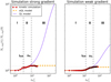 |
Fig. 5. Comparison of the evolution of supra-thermal electron density (tracer of LHDI electron acceleration) computed from full-kinetic simulations (red curve), QL model (blue curve), extended QL model (orange curve). Vertical dashed lines indicate the saturation time tsat, and nonlinear time τNL. Horizontal dotted gray lines indicate the results of Eq. (20). We note that time axes are different for the two simulations. |
First, we observe a minor discrepancy between the two models around t = tsat in the strong gradient case, see Fig. 5 left panel. At this time, the supra-thermal electron density obtained from the full-kinetic simulation (red curve) is higher than that obtained from the QL model (blue curve). This enhanced electron acceleration is due to the overshoot of the electric field in the full-kinetic simulation, an effect that is not included in the QL model and not observed in the weak gradient case. However, this short and sharply peaked phenomenon brings a negligible contribution to the total amount of supra-thermal electrons at the end of the simulation.
Second, we observe a strong discrepancy between the two models for times t > τNL (phase III in Fig. 5). Indeed, on the one hand, the electron acceleration stops at time t ≈ τNL in full-kinetic simulations (red curve) due to the onset of nonlinear LD-like effects, while on the other hand, the electron acceleration goes on in the QL model (blue curve) up to time t ≈ τDiff. The fact that the value of τNL (obtained from full-kinetic simulations) is about one order of magnitude lower than τDiff (obtained from QL simulations) is the main reason for the strong discrepancy between the two models. Such discrepancy is due to the fact that the QL model does not include the nonlinear LD-like effects that are responsible for the abrupt stop of electron acceleration observed at t = τNL in the full-kinetic simulations. Therefore, even though the two models are in good agreement in the linear and quasilinear phases (phases I and II in Fig. 5), the final value of the supra-thermal electron density is strongly overestimated by the QL model. In the following, we use the increase in the supra-thermal electron density, defined as:
 (13)
(13)
to quantify the discrepancy between the models. In particular, the value of ΔNe, sup is 50 (resp. 20) times higher in the strong (resp. weak) gradient case for the QL model as compared to the full-kinetic model.
4.2. Need for an extended quasilinear model
Quasilinear theory is a powerful tool to study wave-particle interaction in an analytical framework due to its relative simplicity. Therefore, it represents an ideal way to provide quantitative predictions on LHDI electron acceleration or heating.
However, due to its derivation via a perturbative approach, QL theory does not include “strong” nonlinear effects (i.e., those effects, arising at sufficiently long times, that alter the wave fluctuations due to the feedback from the modified distribution function to the fields), also called nonlinear LD-like effects. Although they are not included in the QL model, these effects are well self-consistently reproduced by the full-kinetic simulations. The comparison between both models (Sect. 4.1) highlights the need to build an extended QL model (hereafter called eQL) that overcomes the intrinsic limitations of standard QL model and provide a dynamics consistent with that observed in full-kinetic models. For this purpose, we argue that such eQL model: (1) does not require us to include the possible overshoot of the electric field, as we have shown it is not a dominant process in energizing electrons; (2) does require us to include the eventual inhibition of LHDI electron acceleration by nonlinear LD-like effects through the parameter τNL.
The nonlinear time τNL is the parameter used in the eQL to define when nonlinear LD-like effects become dominant in the layer, inhibiting efficient wave-particle interactions. From such time, the QL diffusion coefficient (Eq. (2)) becomes negligible even though the amplitude of the electric field remains constant, as shown in Fig. 6 for both full-kinetic simulations. This is due to its integral dependence on  . The underlying physical process is the energy transfer, in k-space, from resonant, oblique modes to out-of-resonance, more perpendicular modes, which physical mechanism is discussed below. Therefore, we explicitly switch off the QL diffusion coefficient for t > τNL in the eQL model (Eqs. (14) and (15)).
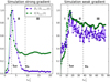 |
Fig. 6. Evolution of the electric field energy S(t)/Smax (green curve), and of the QL diffusion coefficient De(t, vz = 2vthe)/De, max in Eq. (2) (blue curve), computed for both full-kinetic simulations. We note that time axes are different for the two simulations. |
We now focus on the estimation of this new parameter τNL. Previous works on the LHDI addressing its nonlinear evolution using 2D full-kinetic simulations suggest a connection between LHDI modes and drift-kink-instability (fvDKI) modes (Pritchett et al. 1996; Shinohara & Hoshino 1999; Lapenta & Brackbill 2002). The DKI is driven unstable in the presence of a current sheet on a scale length on the order of (or smaller than) the ion gyroradius, as in our full-kinetic simulations setup (see Fig. 1, left panel). The main characteristics of the LHDI are as follows: (i) While the LHDI is an electrostatic instability, the DKI is electromagnetic; (ii) The growth rate of the DKI is much smaller than that of the LHDI: indeed, the DKI frequency and growth rate γDKI are both smaller than the ion gyrofrequency; (iii) The DKI wavevectors are smaller than the inverse of the ion gyroradius; (iv) The DKI modes propagate perpendicular to the magnetic field (Daughton 1998, 1999). In our simulations, the LHDI saturates and start to behave nonlinearly when the DKI is still in its linear stage. As a consequence of the nonlinear dynamics of the LHDI, we observe a coupling between the two instabilities that allows energy to flow from oblique LHDI modes (in their nonlinear stage) to perpendicular DKI modes (in their linear stage). Such a coupling mechanism between LHDI and DKI has been reported and studied in past numerical studies (Pritchett et al. 1996; Shinohara & Hoshino 1999; Lapenta & Brackbill 2002). Therefore, we assume that the mechanism underlying the energy transfer from oblique to strictly perpendicular modes at t > τNL, observed in our full-kinetic simulations, is a LHDI-DKI coupling. Consequently, we estimate that the time of onset of LHDI nonlinear LD-like effects scales as the inverse linear growth rate of the DKI, that is, τNL ∝ 1/γDKI. The DKI linear growth rate, γDKI, scaling with plasma physical parameters has been addressed in Daughton (1998) using kinetic theory, and validated in Daughton (1999) using a two-fluid theory. In our work, we use such results to build our eQL model (Eq. (16)).
Taking all those considerations into account, the eQL model is defined as follows:
 (14)
(14)
 (15)
(15)
 (16)
(16)
where τ0 = 1.5 is a constant obtained from our two full-kinetic simulations. This value is obtained by fitting the evolution of the supra-thermal electron density of the full-kinetic simulations with the one of the eQL model.
4.3. Validation of the extended quasilinear model
The eQL model presented in Sect. 4.2 (Eqs. (14)–(16)) retains all the advantages of the standard QL model (namely being analytical and easily integrable using a numerical solver) while extending its range of validity to asymptotically long time scales. This now enables us to provide quantitative predictions of LHDI electron acceleration. Indeed, as shown by the time evolution of the supra-thermal electron density in Fig. 5, unlike the standard QL predictions (blue), the eQL model (orange) is able to reproduce the predictions of the nonlinear Vlasov-Maxwell theory (red). The relative discrepancy between the two curves does never exceed 5% in both simulations. This validation of the eQL model is of particular interest with regard to quantifying the LHDI electron acceleration over a long time scale.
The results of the eQL model strongly depend on the estimation of the nonlinear time τNL, identified as the inverse linear growth rate of the DKI 1/γDKI. This choice is justified both (i) a priori via previous numerical works that have shown evidence that the long time evolution of a LHDI-unstable layer gets coupled to a DKI (Pritchett et al. 1996; Shinohara & Hoshino 1999); and (ii) a posteriori by validating that the scaling γDKI ∝ (ϵnρi)2 in Eq. (16) is consistent with the outputs of our two full-kinetic simulations.
In our two full-kinetic simulations – which have enabled us to both define and validate the eQL model – we used a reduced ion-to-electron mass ratio mi/me = 100. Using such a reduced mass ratio is standard procedure in PIC plasma simulations since it allows us to reduce the scale separation among the two species in order to run the numerical simulation on reasonable amount of CPU time (still about one million computational hours per simulation, in our case), while maintaining the necessary temporal and spatial scales separations between both species dynamics. However, the properties of the LHDI actually depend on the ion-to-electron mass ratio because of the hybrid character of the instability. Therefore, the quantitative predictions of our full-kinetic simulations are not directly applicable to a realistic plasma configuration (with a physical proton-to-electron mass ratio of 1836). This is exactly where an eQL model becomes extremely useful.
4.4. Using the extended quasilinear model to assess LHDI electron acceleration at physical mass ratio
The eQL model does not suffer from the strong computational constraints of full-PIC simulations and enables us to address, in this section, the question of LHDI electron acceleration using a realistic proton-to-electron mass ratio. The results of the eQL models are summarized in Fig. 7, showing both the electron distribution function evolution averaged in the inhomogeneous layer (top panels) and the resulting supra-thermal electron density (bottom panels), for both strong and weak gradient setups. Here, we use the two setups described in Sect. 2, where only the mass ratio is modified to address the case mi/me = 1836. We emphasize that full kinetic simulations using such a physical mass ratio would have been extremely challenging computationally, so that we consider the eQL model as a way to extrapolate the results of our full-kinetic simulations (done using a reduced mass-ratio) to a physical plasma environment.
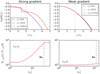 |
Fig. 7. Output of the eQL model using the strong (left panels) and weak (right panels) set of plasma parameters with realistic proton-to-electron mass ratio. Top panels: electron distribution function at different time instants in the direction parallel to the magnetic field. Grey vertical dashed lines correspond to v = 2vthe ≈ vphz. Bottom panels: evolution supra-thermal electron density in Eq. (12). Vertical dashed line indicate the nonlinear time τNL in Eq. (16). Horizontal dotted gray lines indicate the results of Eq. (20). We note that time axes are different for the two simulations. |
Compared to results shown in Sect. 4.3 for a reduced mass ratio, using a physical mass ratio the nonlinear time increases following Eq. (16). This means that the LHW-particle interaction occurs over longer times, thus more electrons are accelerated. However, on the one hand, this effect can be compensated by the reduction of the electric field energy of order ∼me/mi (Eq. (6)) if the LHDI saturates through current relaxation, namely, in the weak gradient case, see Fig. 7 right panel. On the other hand, if the LHDI saturates through ion trapping the saturation level does not depend on the mass-ratio (Eq. (6)); therefore, the LHDI electron acceleration is more efficient by a factor ∼mi/me due to the increase in the nonlinear time.
All in all, the mass ratio does not affect the weak gradient case, while it increases the fraction of LHDI accelerated electrons by a factor ∼1836/100 in the strong gradient case. These predictions – solely based on scaling arguments – are well reproduced by the numerical solution of the eQL using a realistic proton-to-electron mass-ratio, as shown in Fig. 7, and are also confirmed by the analytical estimates developed below in this section.
Now, we focus on the value of the supra-thermal electron density at asymptotically long times, since, all in all, this is the quantity relevant for space plasma observations of LHDI accelerated electrons. Under some simplifying assumptions, we derive an analytical expression for this quantity in the framework of the eQL model.
First, we approximate the evolution of the supra-thermal electron density by a linear interpolation in the time interval tsat < t < τNL to get
 (17)
(17)
then, we integrate Eq. (1) in v∥-space to get
![Mathematical equation: $$ \begin{aligned} \frac{d}{\mathrm{d}t} N_{e,\mathrm{sup}}(t) = \left[ D_e \partial _{ v} f_e \right]_{{ v}_{\parallel }=2{ v}_{\rm the}}, \end{aligned} $$](/articles/aa/full_html/2021/08/aa41049-21/aa41049-21-eq29.gif) (18)
(18)
which is constant in the interval tsat < t < τNL since we assume that (i) the distribution function is weakly modified by the interaction with the wave, that is, fe(t, v∥) ≈ fe(0, v∥), and (ii) the amplitude of the resonant electric field wave |E(k⊥, k∥)| remains constant after the saturation of the LHDI for t > tsat. Finally, under the previous assumptions, using the expression for the QL diffusion coefficient (Eq. (2)) and assuming a Maxwellian distribution function for the electrons, Eqs. (17) and (18) lead us to:
 (19)
(19)
Before going on, we stress here that the increase in supra-thermal density ΔNe, sup is proportional to the amplitude of the electric field at saturation, Smax. This emphasizes how the input parameter Smax/nTi impacts the output of QL theory and further supports the discussion regarding the difference between our results and the ones by Cairns & McMillan (2005) in Sect. 3.2.
Finally, expressing the electric field at saturation Smax using Eq. (6), the nonlinear time, τNL, using Eq. (16), the saturation time, tsat, using Eq. (11), and the LHDI growth rate, γLHDI, using Eq. (5), and under the assumption ωpe > ωce, the supra-thermal density increase in Eq. (19) becomes:
 (20)
(20)
where χ reads:
![Mathematical equation: $$ \begin{aligned} \mathcal \chi = \frac{1.6}{\tau _0} \left(1+\frac{T_e}{T_i}\right)\sqrt{1+\beta _i/2} \ln \left[S_{\max }/S(t=0)\right] . \end{aligned} $$](/articles/aa/full_html/2021/08/aa41049-21/aa41049-21-eq32.gif) (21)
(21)
With the parameters considered in this study, and typically encountered in space plasmas,  . As a consequence, the supra-thermal electron density increase at long times is well approximated analytically by:
 (22)
(22)
depending on the LHDI saturation mechanism at play.
This estimation leads to a total increase in the supra-thermal electron density summarized in Table 1 for the different sets of parameters used throughout this work. These values are also shown as horizontal gray dotted lines in both panels of Fig. 5 – for reduced mass ratio – and Fig. 7 for a physical mass ratio.

From the values in Table 1, we infer that our analytical approximation (Eq. (20)) is valid (error of the order of 10%) in the limit of “weak” LHDI electron acceleration (i.e.,  ). Stronger discrepancies arise for stronger electron acceleration (see third row in Table 1), as expected.
4.5. Application to Mercury’s magnetopause
Mercury’s magnetopause represents an excellent “textbook” example of a plasma boundary with an ion kinetic scale density gradient potentially LHDI-unstable. Previous space missions at Mercury – Mariner 10 (Russell et al. 1988) and MESSENGER (Solomon et al. 2007) – did not bring an instrumental payload capable of providing simultaneous measurements of electric field in the lower-hybrid frequency range and of the electron distribution function. Therefore, the expected LHW physics at Mercury cannot yet be tackled from past observations. However, the physics at these scales is exactly one of the main scientific objectives of the ongoing ESA/JAXA space mission BepiColombo (Benkhoff et al. 2010). Different plasma instruments onboard the Mio spacecraft will provide measurements of: (i) the plasma density profile along the spacecraft trajectory, using different complementary experiments, namely, Langmuir probe measurements (Karlsson et al. 2020), quasi-thermal noise measurements (Moncuquet et al. 2006), and mutual impedance measurements (Gilet et al. 2019), all within the Plasma Wave Investigation (PWI) consortium (Kasaba et al. 2020), (ii) the electric field in the lower-hybrid frequency range (PWI), and (iii) the electron distribution function (MPPE/MEA, Mercury Plasma Particle Experiment and Mercury Electron Analyzer (Saito et al. 2010)). This will enable us to directly address the physics of Mercury’s strongly inhomogeneous magnetopause. In this section, we quantify the expected efficiency of LHDI electron acceleration at Mercury’s magnetopause using the eQL model developed in our work in support for future BepiColombo observations.
As previously pointed out in Sect. 2.2, the parameters used in our strong and weak gradient cases are taken in the range expected at Mercury’s magnetopause (Slavin et al. 2008; Gershman et al. 2015). Therefore, we make use of the results of our eQL model with physical mass ratio in Sect. 4.4 to assess the importance of electron acceleration driven by the LHDI at Mercury’s magnetopause.
First, we discuss the features of the LHW that are expected to be generated by the development of the LHDI at Mercury’s magnetopause. These waves have a frequency of f ≈ fLH ≈ 5–20 Hz (in the frame of the drifting ions) and wavelength λ ≈ 2πρe ≈ 5 − 15 km (hereafter using typical magnetic field values at Mercury’s magnetopause of 10–30 nT, ion temperature 30–70 eV, and density 10–30 cm−3; see Milillo et al. 2020). In the reference frame of the spacecraft, given that those waves are advected by the shocked solar wind flow, estimated to have a speed VSW ≈ 100 km s−1, and with an ion drift speed vDi ≈ vthi ≈ 50 − 80 km s−1, the Doppler-shifted frequency of the LHW, expected to be observed in the spacecraft frame, lies in the range f′=f ± k(vDi + VSW) ≈ 50 − 200 Hz. We note that the Doppler-shifted component is expected to be much higher that the intrinsic frequency, so that the Taylor’s hypothesis is valid for these waves at Mercury’s magnetopause. Moreover, the electric field amplitude of these LHW at saturation is E ≈ 10 − 100 mV m−1, as obtained from Eq. (6). These typical frequency and energy range of LHW at Mercury suggests the use of electric field instruments onboard Mio spacecraft to address the LHW physics at Mercury’s magnetopause. In particular, the sensors MEFISTO and WPT that are part of the PWI consortium (Kasaba et al. 2020) will provide electric field observations in this frequency range with a sensitivity on the order of 10−3 mV m−1, which is well below the expected amplitude of these waves.
Second, we discuss the features of electron distribution functions possibly modified by resonant interaction with the previously discussed LHW. This resonant wave-particle interaction accelerates sub-thermal electrons (with speed vz ⪅ vthe) to supra-thermal energies (with speed vz ⪆ 2vthe) in the direction parallel to the ambient magnetic field, as shown in Fig. 7 top panels. In the following we assume an unperturbed electron temperature of 50 eV (typical values at Mercury’s magnetopause being ∼20 − 100 eV (Ogilvie et al. 1974; Uritsky et al. 2011)). This acceleration process is well in the range of observations of the electron instrument MPPE/MEA onboard the Mio spacecraft of the BepiColombo mission (Saito et al. 2010), since this instrument includes two electron analyzers that can measure the three-dimensional energy distribution of electrons in the range 3–3000 eV (in solar wind mode) or 3–25 500 eV (in magnetospheric mode), with a time resolution of 1 second (Milillo et al. 2020). Here, we simulate the instrumental response of MPPE/MEA when encountering electrons accelerated by a LHDI at Mercury’s magnetopause, as shown in Fig. 8, with the unperturbed electron distribution function in blue, and the one resulting from interaction with LHDI at long times in red. In Fig. 8, the uncertainties on the simulated response of the sensor MEA are obtained using the uncertainty on the G-factor of the instrument reported in Saito et al. (2010) (of the order of 10%). So, on the one hand we predict that the modifications in the electron distribution function above 100 eV are observable by MPPE/MEA in the case of a strongly inhomogeneous magnetopause (width around one ion gyroradius, or less), as shown in the left panel of Fig. 8. On the other hand, since this process is very sensitive to the width of the magnetopause layer, we expect negligible modifications in the electron distribution function for less inhomogeneous magnetopause conditions (width around two ion gyroradii or more), as shown in the right panel of Fig. 8. With typical magnetic field and temperature values at Mercury’s magnetopause the ion gyroradius is around 20 − 80 km.
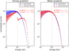 |
Fig. 8. Instrumental response of the instrument MPPE/MEA simulated using our extended QL model for both strong ϵnρi = 1 and weak ϵnρi = 0.5 gradient cases (left and right panels), in the direction parallel to the magnetic field. Unperturbed electron distribution function using temperature Te = 50 eV in blue, and results of eQL model at time t = τNL in red. The dashed vertical line indicates the energy from which the supra-thermal electron density Ne, sup is computed. |
We also assess that the interaction between LHDI and electrons increases both (i) the density of supra-thermal electrons Ne, sup (i.e., electrons with energy higher than 100 eV; see Eq. (12)) and (ii) the electron temperature. In the simulated responses with a strong (resp. weak) density gradient, the former increases by 20% (resp. 0.3%), due to the interaction with the LHW, and the latter increases by 80% (resp. 1.5%). We stress here how these two scalar quantities could be used as tracers of LHDI-electron interaction events in MPPE/MEA data, and how this response is limited to the direction parallel (anti-parallel) to the ambient magnetic field (i.e., around θ = 0° and 180° in the electron pitch-angle distributions).
Third, we present electron observations made by the NASA spacecraft Mariner 10 during its first Mercury flyby on 29 March 1974 (Ogilvie et al. 1974). In Fig. 9, we show the data for the magnetic field (upper panels) and electrons (bottom panels) for the inbound (left) and outbound (right) magnetopause crossings. In particular, we observe a bimodal character of the electron energy distribution during the crossing (bottom panels), with one ambient electron population around 10–30 eV and a second energized population around 100–300 eV. This is consistent with the signatures expected for LHDI-accelerated electrons. Although these observations suggest that the LHDI might play a role in the electron energization at Mercury’s Magnetopause, the Mariner 10 data cannot unambiguously confirm this hypothesis because of the lack of electric field observations. Moreover, the low time resolution of Mariner 10 electron measurements (1/6 s−1), along with the narrow energy range (13.4–687 eV) and the lack of a statistically significant number of crossings mean that the Mariner 10 observations stand in the way of establishing conclusive evidence of LHDI-accelerated electrons at Mercury’s magnetopause.
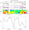 |
Fig. 9. Mariner 10 observations during its first Mercury flyby on the 29 March 1974, inbound (left panels) and outbound (right panels) magnetopause crossings are shown, the associated time intervals are 20:36:30–20:37:30 and 20:53:30–20:54:30, respectively. Magnetosphere (MSP) and magnetosheat (MSH) plasma measurements are shown. From top to bottom, we show the magnetic field module (first row) and its components in MSEQ coordinate (second row) obtained from the magnetometer onboard Mariner 10. Moreover, we show the electron energy spectra as a function of time (third row) and the electron energy spectrum at the time of the crossings (fourth row), obtained from the PLS instrument onboard Mariner 10. The time of the crossings is highlighted by black vertical dashed lines in the first three panels. |
The limits of such Mariner 10 measurements will be overcome by the more advanced and complete payload of the ESA-JAXA BepiColombo space mission, especially the joint electric field observations of LHW (with PWI/MEFISTO and PWI/WPT) and electrons (with MPPE/MEA). We are therefore confident that the Mio plasma and electric field instrumental suites of BepiColombo will soon enable us to shed some light on the statistical relevance of LHDI and associated electron heating in the global dynamics of Mercury’s magnetosphere frontier with the solar wind.
5. Conclusions
In this work, we address the question of electron acceleration efficiency by lower-hybrid waves generated by the lower-hybrid-drift instability.
For this purpose, we have performed 3D, full-kinetic numerical simulations to provide numerical evidence of electrons acceleration parallel to the ambient magnetic field by resonant wave-particle interaction with LHDI waves. Our self-consistent nonlinear model has also enabled us to address the consequences of the saturation of the instability on the eventual stoppage of the electron acceleration. To our the best of our knowledge, this is the first time that this process is self-consistently observed in full-kinetic simulations. This represents the first original contribution of this work.
Moreover, we have provided quantitative estimates of the efficiency of this resonant acceleration process. To model this process, we have (i) used a standard QL model based on the work of Cairns & McMillan (2005), and (ii) developed an extended QL model that includes the consequences of nonlinear LD-like effects on long time scales evolution of the electron distribution function. We compared the results of these two quasilinear models and the full-kinetic model. Such comparison highlighted the limitations at long time scales of the standard quasilinear theory that paved the way for an extended one, designed to overcome such limitations. Such a comparison also enabled us to validate the eQL model. This new extended quasilinear (eQL) model successfully captures the electron acceleration properties found on full-kinetic simulation results and represents the second original contribution of this work.
Thanks to its simplicity, the eQL model has enabled us to explore a range of parameter space that is not accessible to full-kinetic simulations due to computational constraints. In particular, we have addressed the efficiency of LHDI electron acceleration at Mercury’s magnetopause, using a realistic proton-to-electron mass ratio. In this context, we estimate that LHDI electron acceleration is an efficient mechanism for energizing electrons during periods of strong magnetospheric compression (when the magnetopause boundary steepens on scales of the order or lower than the ion gyroradius). This efficiency strongly depends on the density gradient at the magnetopause. Under such conditions of a “steep” magnetopause at Mercury, we expect strong signatures of LHDI electron acceleration in the BepiColombo instrumental suite response (PWI and MPPE/MEA).
We are confident that our extended quasilinear model will enable quantitative studies of the efficiency of electron acceleration in inhomogeneous space plasmas in support of past and future space plasma observations. More importantly, this work also provides a validated framework for extending the range of the validity and applicability of quasilinear modeling, not only associated with the lower-hybrid-drift instability – as in this study – but also to a broader variety of waves and instabilities in space plasmas.
Acknowledgments
The authors thank the referee for useful comments and suggestions. This study was granted access to the HPC resources of SIGAMM infrastructure (http://crimson.oca.eu), hosted by Observatoire de la Côte d’Azur and which is supported by the Provence-Alpes Côte d’Azur region. This work was performed using HPC resources from GENCI-CINES (Grants 2020-A0080411496, 2021-A0100412428). We acknowledge PRACE for awarding us access to Joliot-Curie at GENCI@CEA, France. We acknowledge the CINECA award under the ISCRA initiative, for the availability of high performance computing resources and support for the project IsC71. We acknowledge the computing center of Cineca and INAF, under the coordination of the “Accordo Quadro MoU per lo svolgimento di attivitá congiunta di ricerca Nuove frontiere in Astrofisica: HPC e Data Exploration di nuova generazione”, for the availability of computing resources and support. The authors would like to thank the Smilei team for their brilliant technical support (https://smileipic.github.io/Smilei), and in particular Mickael Grech for the fruitful discussions. Data analysis was performed with the AMDA science analysis system provided by the Centre de Données de la Physique des Plasmas (CDPP) supported by CNRS, CNES, Observatoire de Paris and Université Paul Sabatier, Toulouse. The Mariner 10 data is also available on the Planetary Data System (https://pds.nasa.gov). We acknowledge the support of CNES for the BepiColombo mission.
References
- Alexandrov, A. F., Bogdankevich, L. S., & Rukhadze, A. A. 1984, Principles of Plasma Electrodynamics, Series in Electrophysics (Springer) [CrossRef] [Google Scholar]
- Alpers, W. 1969, Ap&SS, 5, 425 [CrossRef] [Google Scholar]
- Amatucci, W. E. 1999, J. Geophys. Res., 104, 14481 [CrossRef] [Google Scholar]
- André, M., Behlke, R., Wahlund, J. E., et al. 2001, Ann. Geophys., 19, 1471 [CrossRef] [Google Scholar]
- André, M., Odelstad, E., Graham, D., et al. 2017, MNRAS, 469 [Google Scholar]
- Bale, S. D., Mozer, F. S., & Phan, T. 2002, Geophys. Res. Lett., 29, 33 [CrossRef] [Google Scholar]
- Bécoulet, A., Hoang, G., Artaud, J., et al. 2011, Fusion Eng. Des., 86, 490 [CrossRef] [Google Scholar]
- Benkhoff, J., van Casteren, J., Hayakawa, H., et al. 2010, Planet. Space Sci., 58, 2 [NASA ADS] [CrossRef] [Google Scholar]
- Bernstein, I. B., & Engelmann, F. 1966, Phys. Fluids, 9, 937 [CrossRef] [Google Scholar]
- Bingham, R., Dawson, J. M., & Shapiro, V. D. 2002, J. Plasma Phys., 68, 161 [NASA ADS] [CrossRef] [Google Scholar]
- Birdsall, C. K., & Langdon, A. B. 1991, Plasma Physics via Computer Simulation (Adam Hilger IOP Publishing) [CrossRef] [Google Scholar]
- Brackbill, J. U., Forslund, D. W., Quest, K. B., & Winske, D. 1984, Phys. Fluids, 27, 2682 [CrossRef] [Google Scholar]
- Broiles, T. W., Burch, J. L., Chae, K., et al. 2016, MNRAS, 462, S312 [CrossRef] [Google Scholar]
- Brunetti, M., Califano, F., & Pegoraro, F. 2000, Phys. Rev. E, 62, 4109 [NASA ADS] [CrossRef] [Google Scholar]
- Cairns, I. H., & McMillan, B. F. 2005, Phys. Plasmas, 12 [Google Scholar]
- Chen, Y., & Birdsall, C. K. 1983, Phys. Fluids, 26, 180 [CrossRef] [Google Scholar]
- Daughton, W. 1998, J. Geophys. Res., 103, 29429 [CrossRef] [Google Scholar]
- Daughton, W. 1999, J. Geophys. Res., 104, 28701 [CrossRef] [Google Scholar]
- Daughton, W. 2003, Phys. Plasmas, 10, 3103 [CrossRef] [Google Scholar]
- Davidson, R. C. 1978, Phys. Fluids, 21, 1375 [CrossRef] [Google Scholar]
- Davidson, R. C., Gladd, N. T., Wu, C. S., & Huba, J. D. 1977, Phys. Fluids, 20, 301 [CrossRef] [Google Scholar]
- Derouillat, J., Beck, A., Pérez, F., et al. 2018, Comput. Phys. Commun., 222, 351 [CrossRef] [Google Scholar]
- Gary, S. P. 1993, Theory of Space Plasma Microinstabilities, Cambridge Atmospheric and Space Science Series (Cambridge University Press) [Google Scholar]
- Gary, S. P., & Sanderson, J. J. 1978, Phys. Fluids, 21, 1181 [CrossRef] [Google Scholar]
- Gary, S. P., & Sgro, A. G. 1990, Geophys. Res. Lett., 17, 909 [CrossRef] [Google Scholar]
- Gershman, D. J., Raines, J. M., Slavin, J. A., et al. 2015, J. Geophys. Res.: Space Phys., 120, 4354 [CrossRef] [Google Scholar]
- Gilet, N., Henri, P., Wattieaux, G., et al. 2019, Front. Astron. Space Sci., 6, 16 [CrossRef] [Google Scholar]
- Goldstein, R., Burch, J. L., Llera, K., et al. 2019, A&A, 630, A40 [CrossRef] [EDP Sciences] [Google Scholar]
- Graham, D. B., Khotyaintsev, Y. V., Norgren, C., et al. 2019, J. Geophys. Res.: Space Phys., 124, 8727 [CrossRef] [Google Scholar]
- Graham, D. B., Khotyaintsev, Y. V., Norgren, C., et al. 2017, J. Geophys. Res.: Space Phys., 122, 517 [CrossRef] [Google Scholar]
- Hoshino, M., Mukai, T., Terasawa, T., & Shinohara, I. 2001, J. Geophys. Res., 106, 25979 [NASA ADS] [CrossRef] [Google Scholar]
- Huba, J., Gladd, T., & Papadopoulos, K. 1978, J. Geophys. Res., 83 [Google Scholar]
- Karlsson, T., Eriksson, A. I., Odelstad, E., et al. 2017, Geophys. Res. Lett., 44, 1641 [NASA ADS] [Google Scholar]
- Karlsson, T., Kasaba, Y., Wahlund, J.-E., et al. 2020, Space Sci. Rev., 216 [Google Scholar]
- Kasaba, Y., Kojima, H., Moncuquet, M., et al. 2020, Space Sci. Rev., 216, 65 [CrossRef] [Google Scholar]
- Khotyaintsev, Y. V., Cully, C. M., Vaivads, A., André, M., & Owen, C. J. 2011, Phys. Rev. Lett., 106, 165001 [NASA ADS] [CrossRef] [Google Scholar]
- Krall, N. A., & Liewer, P. C. 1971, Phys. Rev. A, 4, 2094 [CrossRef] [Google Scholar]
- Krall, N. A., & Trivelpiece, A. W. 1973, Principles of Plasma Physics (McGraw-Hill) [Google Scholar]
- Krasnoselskikh, V. V., Kruchina, E. N., Volokitin, A. S., & Thejappa, G. 1985, A&A, 149, 323 [Google Scholar]
- Laming, J. M. 2001, ApJ, 563, 828 [NASA ADS] [CrossRef] [Google Scholar]
- Lapenta, G., & Brackbill, J. U. 2002, Phys. Plasmas, 9, 1544 [CrossRef] [Google Scholar]
- Lapenta, G., Brackbill, J. U., & Daughton, W. S. 2003, Phys. Plasmas, 10, 1577 [CrossRef] [Google Scholar]
- Lapenta, G., Pucci, F., Olshevsky, V., et al. 2018, J. Plasma Phys., 84, 715840103 [CrossRef] [Google Scholar]
- Le Contel, O., Nakamura, R., Breuillard, H., et al. 2017, J. Geophys. Res.: Space Phys., 122, 12,236 [CrossRef] [Google Scholar]
- Markidis, S., Lapenta, G., & Rizwan-uddin 2010, Math. Comput. Simul., 80, 1509 [CrossRef] [Google Scholar]
- McBride, J., & Ott, E. 1972, Phys. Lett. A, 39, 363 [CrossRef] [Google Scholar]
- McBride, J. B., Ott, E., Boris, J. P., & Orens, J. H. 1972, Phys. Fluids, 15, 2367 [CrossRef] [Google Scholar]
- McClements, K. G., Bingham, R., Su, J. J., Dawson, J. M., & Spicer, D. S. 1993, ApJ, 409, 465 [NASA ADS] [CrossRef] [Google Scholar]
- McMillan, B. F. 2020, Phys. Plasmas, 27, 052106 [CrossRef] [Google Scholar]
- Milillo, A., Fujimoto, M., Murakami, G., et al. 2020, Space Sci. Rev., 216, 93 [CrossRef] [Google Scholar]
- Moncuquet, M., Matsumoto, H., Bougeret, J. L., et al. 2006, Adv. Space Res., 38, 680 [Google Scholar]
- Norgren, C., Vaivads, A., Khotyaintsev, Y. V., & André, M. 2012, Phys. Rev. Lett., 109, 055001 [NASA ADS] [CrossRef] [Google Scholar]
- Ogilvie, K. W., Scudder, J. D., Hartle, R. E., et al. 1974, Science, 185, 145 [CrossRef] [Google Scholar]
- Ott, E., McBride, J. B., Orens, J. H., & Boris, J. P. 1972, Phys. Rev. Lett., 28, 88 [NASA ADS] [CrossRef] [Google Scholar]
- Pericoli-Ridolfini, V., Barbato, E., Cirant, S., et al. 1999, Phys. Rev. Lett., 82, 93 [CrossRef] [Google Scholar]
- Pritchett, P. L., Coroniti, F. V., & Decyk, V. K. 1996, J. Geophysical. Res.: Space Phys., 101, 27413 [CrossRef] [Google Scholar]
- Pu, Z.-Y., Quest, K. B., Kivelson, M. G., & Tu, C.-Y. 1981, J. Geophys. Res.: Space Phys., 86, 8919 [CrossRef] [Google Scholar]
- Reiniusson, A., Stenberg, G., Norqvist, P., Eriksson, A. I., & Rönnmark, K. 2006, Ann. Geophys., 24, 367 [CrossRef] [Google Scholar]
- Retinó, A., Nakamura, R., Vaivads, A., et al. 2008, J. Geophys. Res.: Space Phys., 113 [Google Scholar]
- Rigby, A., Cruz, F., Albertazzi, B., et al. 2018, Nat. Phys., 14, 475 [CrossRef] [Google Scholar]
- Russell, C. T., Baker, D. N., & Slavin, J. A. 1988, The Magnetosphere of Mercury (NTRS), 514 [Google Scholar]
- Sagdeev, R. Z., Shapiro, V. D., Shevchenko, V. I., et al. 1990, Geophys. Res. Lett., 17, 893 [CrossRef] [Google Scholar]
- Saito, Y., Sauvaud, J. A., Hirahara, M., et al. 2010, Planet. Space Sci., 58, 182 [NASA ADS] [CrossRef] [Google Scholar]
- Scarf, F. L., Taylor, W. W. L., Russell, C. T., & Elphic, R. C. 1980, J. Geophys. Res.: Space Phys., 85, 7599 [CrossRef] [Google Scholar]
- Shapiro, V. D., Szegö, K., Ride, S. K., Nagy, A. F., & Shevchenko, V. I. 1995, J. Geophys. Res., 100, 21289 [NASA ADS] [CrossRef] [Google Scholar]
- Shapiro, V. D., Bingham, R., Dawson, J. M., et al. 1999, J. Geophys. Res.: Space Phys., 104, 2537 [NASA ADS] [CrossRef] [Google Scholar]
- Shinohara, I., & Hoshino, M. 1999, Adv. Space Res., 24, 43 [CrossRef] [Google Scholar]
- Singh, N., Al-Sharaeh, S., Abdelrazek, A., Leung, W. C., & Wells, B. E. 1996, Geophys. Res. Lett., 23, 3663 [CrossRef] [Google Scholar]
- Singh, N., Wells, B. E., Abdelrazek, A., Al-Sharaeh, S., & Leung, W. C. 1998, J. Geophys. Res., 103, 9333 [CrossRef] [Google Scholar]
- Slavin, J. A., Acuña, M. H., Anderson, B. J., et al. 2008, Science, 321, 85 [NASA ADS] [CrossRef] [Google Scholar]
- Solomon, S. C., McNutt, R. L., Gold, R. E., & Domingue, D. L. 2007, Space Sci. Rev., 131, 3 [NASA ADS] [CrossRef] [Google Scholar]
- Tang, B. B., Li, W. Y., Graham, D. B., et al. 2020, Geophys. Res. Lett., 47, e89880 [Google Scholar]
- Uritsky, V. M., Slavin, J. A., Khazanov, G. V., et al. 2011, J. Geophys. Res.: Space Phys., 116 [Google Scholar]
- Vaivads, A., André, M., Buchert, S. C., et al. 2004, Geophys. Res. Lett., 31, L03804 [CrossRef] [Google Scholar]
- Walker, S. N., Balikhin, M. A., Alleyne, H. S. C. K., et al. 2008, Ann. Geophys., 26, 699 [CrossRef] [Google Scholar]
- Wilson, L. B., Koval, A., Szabo, A., et al. 2013, J. Geophys. Res. (Space Phys.), 118, 5 [CrossRef] [Google Scholar]
- Winske, D., & Liewer, P. C. 1978, Phys. Fluids, 21, 1017 [CrossRef] [Google Scholar]
- Yoo, J., Ji, J.-Y., Ambat, M. V., et al. 2020, Geophys. Res. Lett., 47 [Google Scholar]
- Zacharegkas, G., Isliker, H., & Vlahos, L. 2016, Phys. Plasmas, 23, 112119 [CrossRef] [Google Scholar]
- Zhang, Y., & Matsumoto, H. 1998, J. Geophys. Res.: Space Phys., 103, 20561 [CrossRef] [Google Scholar]
- Zhou, M., Deng, X. H., Li, S. Y., et al. 2009, J. Geophys. Res.: Space Phys., 114 [Google Scholar]
- Zhou, M., Li, H., Deng, X., et al. 2014, J. Geophys. Res.: Space Phys., 119, 8228 [CrossRef] [Google Scholar]
All Tables
All Figures
|
Fig. 1. Schematic view of the setup of the full-kinetic 3D-3V simulations presented in this study. Left panel: Density, magnetic field, and current profiles at t = 0 along the direction of the inhomogeneity (x-axis) in the “strong gradient” simulation. Right panel: 3D visualization of the ion density in the “strong gradient” simulation at |
| In the text | |
|
Fig. 2. Saturation mechanisms at play in the two simulations: ion trapping (left panels) and current relaxation (right panel). Left panels: isocontour of the ion phase space density (top panel) together with the electric potential of the LHDI waves (bottom panel) on the same spatial axis, both quantities being computed in the unstable layer. Right panel: evolution of the difference between the average charged current in the unstable layer (2 < x < 4) and its value at t = 0, for both simulations. |
| In the text | |
|
Fig. 3. Full-kinetic simulations: evolution of the electron supra-thermal density Ne, sup(t)/Ne, sup(0) (red curves) and of the electric field energy normalized to the ion thermal energy S/nTi(t) (green curves), both curves are integrated over the unstable layer (3.5 < x < 4 for strong gradient and 3.5 < x < 4.5 for weak gradient). We note that time axes are different for the two simulations. |
| In the text | |
|
Fig. 4. Results of the QL model for the strong and weak gradient parameter case, shown in the left and right panel, respectively. Both panels show the electron distribution function at different time instants in the direction parallel to the magnetic field. Grey vertical dashed lines at v = 2vthe ≈ vphz correspond to the point from where the supra-thermal electron density (Eq. (12)) is computed. |
| In the text | |
|
Fig. 5. Comparison of the evolution of supra-thermal electron density (tracer of LHDI electron acceleration) computed from full-kinetic simulations (red curve), QL model (blue curve), extended QL model (orange curve). Vertical dashed lines indicate the saturation time tsat, and nonlinear time τNL. Horizontal dotted gray lines indicate the results of Eq. (20). We note that time axes are different for the two simulations. |
| In the text | |
|
Fig. 6. Evolution of the electric field energy S(t)/Smax (green curve), and of the QL diffusion coefficient De(t, vz = 2vthe)/De, max in Eq. (2) (blue curve), computed for both full-kinetic simulations. We note that time axes are different for the two simulations. |
| In the text | |
|
Fig. 7. Output of the eQL model using the strong (left panels) and weak (right panels) set of plasma parameters with realistic proton-to-electron mass ratio. Top panels: electron distribution function at different time instants in the direction parallel to the magnetic field. Grey vertical dashed lines correspond to v = 2vthe ≈ vphz. Bottom panels: evolution supra-thermal electron density in Eq. (12). Vertical dashed line indicate the nonlinear time τNL in Eq. (16). Horizontal dotted gray lines indicate the results of Eq. (20). We note that time axes are different for the two simulations. |
| In the text | |
|
Fig. 8. Instrumental response of the instrument MPPE/MEA simulated using our extended QL model for both strong ϵnρi = 1 and weak ϵnρi = 0.5 gradient cases (left and right panels), in the direction parallel to the magnetic field. Unperturbed electron distribution function using temperature Te = 50 eV in blue, and results of eQL model at time t = τNL in red. The dashed vertical line indicates the energy from which the supra-thermal electron density Ne, sup is computed. |
| In the text | |
|
Fig. 9. Mariner 10 observations during its first Mercury flyby on the 29 March 1974, inbound (left panels) and outbound (right panels) magnetopause crossings are shown, the associated time intervals are 20:36:30–20:37:30 and 20:53:30–20:54:30, respectively. Magnetosphere (MSP) and magnetosheat (MSH) plasma measurements are shown. From top to bottom, we show the magnetic field module (first row) and its components in MSEQ coordinate (second row) obtained from the magnetometer onboard Mariner 10. Moreover, we show the electron energy spectra as a function of time (third row) and the electron energy spectrum at the time of the crossings (fourth row), obtained from the PLS instrument onboard Mariner 10. The time of the crossings is highlighted by black vertical dashed lines in the first three panels. |
| In the text | |
Current usage metrics show cumulative count of Article Views (full-text article views including HTML views, PDF and ePub downloads, according to the available data) and Abstracts Views on Vision4Press platform.
Data correspond to usage on the plateform after 2015. The current usage metrics is available 48-96 hours after online publication and is updated daily on week days.
Initial download of the metrics may take a while.