| Issue |
A&A
Volume 651, July 2021
|
|
|---|---|---|
| Article Number | A93 | |
| Number of page(s) | 20 | |
| Section | Planets and planetary systems | |
| DOI | https://doi.org/10.1051/0004-6361/202141141 | |
| Published online | 21 July 2021 | |
HADES RV programme with HARPS-N at TNG
XIV. A candidate super-Earth orbiting the M-dwarf GJ 9689 with a period close to half the stellar rotation period★,★★
1
INAF – Osservatorio Astronomico di Palermo,
Piazza del Parlamento 1,
90134
Palermo,
Italy
e-mail: jesus.maldonado@inaf.it
2
INAF – Osservatorio Astrofisico di Torino,
Via Osservatorio 20,
10025
Pino Torinese,
Italy
3
INAF – Osservatorio Astrofisico di Catania,
Via S. Sofia 78,
95123
Catania,
Italy
4
Centro de Astrobiología (CSIC-INTA),
Carretera de Ajalvir km 4,
28850
Torrejón de Ardoz,
Madrid,
Spain
5
Fundación Galileo Galilei-INAF,
Rambla José Ana Fernández Pérez 7,
38712
Breña Baja,
TF,
Spain
6
INAF – Osservatorio Astronomico di Brera,
Via E. Bianchi 46,
23807
Merate,
Italy
7
Institut de Ciéncies de l’Espai (ICE, CSIC),
Campus UAB, Carrer de Can Magrans s/n,
08193
Bellaterra,
Spain
8
Institut d’Estudis Espacials de Catalunya (IEEC),
08034
Barcelona,
Spain
9
Instituto de Astrofísica de Canarias,
38205
La Laguna,
Tenerife,
Spain
10
Universidad de La Laguna, Departamento Astrofísica,
38206
La Laguna,
Tenerife,
Spain
11
INAF – Osservatorio Astronomico di Trieste,
Via Tiepolo 11,
34143
Trieste,
Italy
12
INAF – Osservatorio Astronomico di Cagliari and REM,
Via della Scienza, 5,
09047
Selargius
CA,
Italy
13
INAF – Osservatorio Astronomico di Capodimonte,
Salita Moiariello 16,
80131
Napoli,
Italy
14
INAF – Osservatorio Astronomico di Padova,
vicolo dell’Osservatorio 5,
35122
Padova,
Italy
15
Dipartimento di Fisica e Astronomia Galileo Galilei,
Vicolo Osservatorio 3,
35122
Padova,
Italy
Received:
20
April
2021
Accepted:
12
May
2021
Context. It is now well-established that small, rocky planets are common around low-mass stars. However, the detection of such planets is challenged by the short-term activity of host stars.
Aims. The HARPS-N red Dwarf Exoplanet Survey programme is a long-term project at the Telescopio Nazionale Galileo aimed at monitoring nearby, early-type, M dwarfs, using the HARPS-N spectrograph to search for small, rocky planets.
Methods. A total of 174 HARPS-N spectroscopic observations of the M0.5V-type star GJ 9689 taken over the past seven years have been analysed. We combined these data with photometric measurements to disentangle signals related to the stellar activity of the star from possible Keplerian signals in the radial velocity data. We ran an MCMC analysis, applying Gaussian process regression techniques to model the signals present in the data.
Results. We identify two periodic signals in the radial velocity time series, with periods of 18.27 and 39.31 d. The analysis of the activity indexes, photometric data, and wavelength dependency of the signals reveals that the 39.31 d signal corresponds to the stellar rotation period. On the other hand, the 18.27 d signal shows no relation to any activity proxy or the first harmonic of the rotation period. We, therefore, identify it as a genuine Keplerian signal. The best-fit model describing the newly found planet, GJ 9689 b, corresponds to an orbital period of Pb = 18.27 ± 0.01 d and a minimum mass of MP sini = 9.65 ± 1.41 M⊕.
Key words: techniques: spectroscopic / techniques: radial velocities / stars: late-type / planetary systems / stars: individual: GJ 9689
Table A.1 is only available in electronic form at the CDS via anonymous ftp to cdsarc.u-strasbg.fr (130.79.128.5) or via http://cdsarc.u-strasbg.fr/viz-bin/cat/J/A+A/651/A93
© ESO 2021
1 Introduction
Starting with the first exoplanet discoveries (Wolszczan & Frail 1992; Mayor & Queloz 1995), astronomers have succeeded in unravelling an astonishing diversity of planetary systems, compositions, and host stellar properties (e.g. Udry & Santos 2007; Cumming 2010; Howard 2013; Perryman 2018). Low-mass stars or M dwarfs constitute the most common stellar component in the Milky Way (e.g. Chabrier & Baraffe 2000). However, unlike their FGK counterparts, results regarding the properties of planets around M dwarfs still focus on small sample sizes and suffer from the intrinsic difficulties in the spectral characterisation of M dwarfs. In spite of their high levels of stellar variability and their intrinsic faintness at optical wavelengths, it is now widely accepted that low-mass stars are optimal targets around which to search for small rocky planets (e.g. Dressing & Charbonneau 2013, 2015) and a large number of radial velocity (RV) and photometric surveys are currently focused on M dwarfs. Some examples include the HET and HPF M dwarf surveys (Endl et al. 2003; Wright et al. 2018), the HARPS-GTO programme (Bonfils et al. 2013), the HADES survey (Affer et al. 2016), CARMENES (e.g. Zechmeister et al. 2019), SPIRou (e.g. Klein et al. 2021), SOPHIE (e.g. Hobson et al. 2019), the MEarth project (Nutzman & Charbonneau 2008), APACHE (Sozzetti et al. 2013), TRAPPIST (Gillon, M. et al. 2012), and TESS (e.g. Feliz et al. 2021).
At the time of writing this paper, there are ~130 known RV planets around M dwarfs listed in the Extrasolar Planets Encyclopaedia (Schneider et al. 2011)1, and several interesting trends regarding the properties of planets around M dwarfs have already been discussed. It has been established that, unlike their solar-type counterparts, the frequency of gas-giant planets orbiting low-mass stars is low (Endl et al. 2003, 2006; Butler et al. 2006; Bonfils et al. 2007; Cumming et al. 2008; Johnson et al. 2010). On the other hand, as found for FGK stars, small planets orbiting M dwarfs seem to be very abundant, most of them being in multi-planet systems. The HARPS-M dwarf survey reports a 36% occurrence for super-Earths (Mp sini < 10 M⊕) in short periods (P < 10 d) and 52% for 10 days < P < 100 d (Bonfils et al. 2013). Tuomi et al. (2014) estimate a frequency of low-mass planets around M dwarfs of one planet per star, possibly even greater. Results from the KEPLER mission suggest that the frequency of planets (with periods below 50 days) around stars seems to increase as we move from F stars towards the M dwarf type (Howard et al. 2012). Along this line, Mann et al. (2012) report an occurrence rate of super-Earths with periods lower than 50 days of 36 ± 8% around late-K to early M dwarfs.
The frequency of planets around M dwarfs seems to follow the same stellar mass and metallicity trends as FGK stars. That is to say, the frequency of gas-giant planets is a function of the stellar metallicity as well as of the stellar mass. On the other hand, the frequency of low-mass planets does not depend on the metallicity content or the mass of the stellar host (Bonfils et al. 2007; Johnson & Apps 2009; Schlaufman & Laughlin 2010; Rojas-Ayala et al. 2012; Terrien et al. 2012; Neves et al. 2013; Montet et al. 2014; Courcol et al. 2016; Maldonado et al. 2020). While most studies have focused only on the iron contentor metallicity, in a recent work, Maldonado et al. (2020) show, for the first time, that there are no differences in the abundance distribution of elements other than iron between M dwarfs with and without known planets.
The detection of truly Earth twins via the Doppler technique requires a precision in the RV measurements of the order of 0.1 ms-1. While a new generation of ultra high-resolution spectrographs is coming to the forefront (e.g. ESPRESSO Pepe et al. 2021), it is now clear that the major challenge to high Doppler precision is not the instrumental precision, but the star itself. Stellar activity might produce line profile variations that skew the peak of a spectral line, leading to a velocity change in the star that can be (mis)interpreted as Keplerian in nature. (Saar & Donahue 1997; Santos et al. 2000; Paulson et al. 2004; Wright 2005; Desort et al. 2007; Dumusque et al. 2011a). Some techniques such as an optimal schedule of the observations or the use of spectroscopic indicators of activity might be used to mitigate the effects of stellar oscillations, granulation, or even long-term activity (Dumusque et al. 2011a,b). However, the short-term stellar activity, due to the evolution and decay of active regions, has a characteristic timescale comparable with the stellar rotation period (e.g. Scandariato et al. 2017). Disentangling ‘true’ Keplerian signals from stellar variations is highly complex and requires the use of complementary and imaginative approaches, such as red-noise models or Gaussian process regression (see e.g. Dumusque et al. 2017, and references therein).
Within the framework of the HARPS-N red Dwarf Exoplanet Survey (HADES) observing programme (Affer et al. 2016), we have started the RV monitoring of a large sample of low-mass stars (spectral types K7-M3). The main goal of HADES is to explore the frequency and formation conditions of small, potentially habitable planets around early-M dwarfs. The development of techniques to ensure the optimal outcome of the survey is an additional goal of HADES, and it includes target characterisation (Maldonado et al. 2015, 2020), optimal scheduling (Perger et al. 2017a), or detailed activity studies (Maldonado et al. 2017; Scandariato et al. 2017; Suárez Mascareño et al. 2018; González-Álvarez et al. 2019). HADES has already succeeded in discovering several super-Earth exoplanets, with masses ranging from 2.5 M⊕ to 9 M⊕ (Affer et al. 2016; Suárez Mascareño et al. 2017; Perger et al. 2017b; Pinamonti et al. 2018, 2019; Affer et al. 2019; Perger et al. 2019; Toledo-Padrón et al. 2021; González-Álvarez et al. 2021).
In this paper we present the discovery of a candidate super-Earth (Mp sini ~9.65 M⊕) planet orbiting around the early-M dwarf GJ 9689 with a period of 18.27 d. The detection of this planet has been challenging, as the proposed planetary period is very close to half the stellar rotation period (39.31 d). This fact makes the GJ 9689 b planet an interesting case of study. This paper is organised as follows. Section 2 reviews the stellar properties of GJ 9689. The spectroscopic data are presented in Sect. 3, while Sect. 4 describes the analysis of the RV data. The origin of the RV variations found in GJ 9689 is discussed at length in Sect. 5, where activity indicators, photometry,and CCF diagnostics are analysed. Section 6 describes the modelling of the RV variations. The results are set in the context of planetary systems in Sect. 7. Our conclusions follow in Sect. 8.
2 The host star
GJ 9689 is an M0.5 dwarf located at a distance of 30.69 ± 0.01 pc (Gaia Collaboration 2020) from the Sun. Its main stellar properties are listed in Table 1. Basic stellar parameters (effective temperature, spectral type, mass, radius, surface gravity, and luminosity) are from Maldonado et al. (2020). They were computed following the procedures described in Maldonado et al. (2015)2, which make use of the same spectra used in this work for the RV analysis. In brief, effective temperatures and spectral types were determined from ratios of pseudo-equivalent widths of spectral features calibrated using stars with interferometric estimates of their radii and spectral-type standards. By studying a large sample of early-M dwarfs, Maldonado et al. (2015) also provide empirical calibrations for the stellar mass, radius, and surface gravity as a function of the stellar metallicity and effective temperature. Stellar metallicity was computed by a methodology based on the use of a principal component analysis andsparse Bayesian methods, which also allows for the determination of abundances of other elements different from iron3 (Maldonado et al. 2020). These parameters are listed for the whole HADES sample in Maldonado et al. (2017) and for a large sample of Mdwarfs in current RV searches in Maldonado et al. (2020).
Galactic spatial-velocity components (U, V, W) were computed from the RVs, together with Gaia parallaxes and proper motions (Gaia Collaboration 2020), following the procedure described in Montes et al. (2001) and Maldonado et al. (2010). GJ 9689 is classified as a transition star (its kinematical properties lie in between the definitions of the thin and thick disk populations) applying the methodology described in Bensby et al. (2003, 2005). No comoving objects seems to be present after carefully checking the available data in the Gaia EDR3 catalogue.
Physical properties of GJ 9689.
3 Spectroscopic observations
GJ 9689 has been observed for a period of almost seven and a half years, from BJD = 2 5456 438 (May 26, 2013) toBJD = 2 459 130 (October 7, 2020). A total of 174 HARPS-N observations were collected during this period. HARPS-N spectra cover the wavelength range 383–693 nm with a resolving power of R ~115 000. Data were reduced using the latest version of the Data Reduction Software (DRS V3.7, Lovis & Pepe 2007), which implements the typical corrections involved in échelle spectra reduction, that is to say bias level correction, flat-fielding, order extraction, wavelength calibration, and merging individual orders. RVs are computed by cross-correlating the spectra of the target star with an optimised binary mask (Baranne et al. 1996; Pepe et al. 2002). For GJ 9689, the M2 mask was used. This procedure is known to have several shortcomings firstly since a symmetric analytical function is used to fit the asymmetric CCF. Furthermore, spectra of an M dwarf suffer from heavy blends, resulting in side-lobes in the CCF which might affect the RV precision as well as the asymmetry indexes of the CCF (e.g. Rainer et al. 2020). In order to overcome these difficulties, RVs were also computed with the Java-based Template-Enhanced Radial velocity Re-analysis Application (TERRA, Anglada-Escudé & Butler 2012). TERRA measures the RVs by a least-square match of each observed spectrum to a co-added high signal-to-noise ratio (S/N) template spectra derived from the same observations. We excluded the bluest part of the spectra from the analysis and only orders redder than the 22nd (λ > 453 nm) were considered (we note that HARPS-N spectra have a total of 66 échelle orders).
4 RV time series analysis
Figure 1 (top) shows the RV (derived with the TERRA pipeline) time series of GJ 9689. The RV data show a root mean square (rms) of 4.59 m s-1, approximately 3 times the mean error of the measured RVs (1.55 m s-1) when the TERRA pipeline is used. If the RV data are derived by the DRS then we obtain a rms of 5.35 m s-1, while the mean error of the measured RVs is 2.94 m s-1.
In a recent work, Perger et al. (2017a) performed a detailed comparison on the accuracy of the TERRA and DRS pipelines using the HADES spectra collected so far. Under the assumption that a smaller rms of the RV measurements correspond to a smaller RV noise rms, the authors conclude that TERRA RVs should be preferred. In particular, for GJ 9689, the rms of the RV measurements obtained with TERRA is around 1 ms-1 lower than the value derived by the DRS RVs. The analysis presented in the following refers to TERRA RVs.
A search for periodicities in the RV data was performed by using the generalised Lomb-Scargle periodogram (GLS, Zechmeister & Kürster 2009). The periodogram (see Fig. 2) identifies two significant frequencies. The peaks are found at 0.054734 ± 0.000039 d-1 (period of 18.27 ± 0.01 d) and 0.025436 ± 0.000059 d-1, which corresponds to a period of 39.31 ± 0.10 d. In order to test the significance of these frequencies, a bootstraping analysis was carried out. A series of 104 simulations was performed. In each simulation the dates of the observed RVs were kept, but random RVs were constructed from the original ones by drawing random values from normal distributions with means equals to the RV value and σ equal to the RV error. Then, the simulated RVs were randomly shuffled. The false alarm probability (FAP) of a given period is obtained as the fraction of simulated periodograms in which a peak with a periodogram power larger than the original period’s power is found (e.g. Endl et al. 2001). Both signals are found to have a FAP below the 0.1% threshold.
We performed a search for additional periods by subtracting the most prominent period in a sequential way until no significant signal was left, a procedure usually known as pre-whitening. First of all, a sinusoidal function with a period of 18.27 d was fitted and subtracted. It can be seen from the periodogram (middle panel of Fig. 2) that the period at 39.31 d is still significant after the removal of the 18.27 d signal. Once the 39.31 d signal is also subtracted, no significant periods remain in the periodogram analysis (bottom panel of Fig. 2). We note that the peak with the highest power seems to be the harmonic of the 39.31 d signal as it is located at a frequency of 0.050364 ± 0.000075 d-1, which corresponds to a period of 19.86 ± 0.03 d.
We note that if the 39.31 d signal is firstly pre-whitened from the raw RV dataset, then the 18.27 d signal clearly remains (Fig. 3). That suggests that both signals are not connected. For the sake of completeness, we also show the GLS periodogram derived using the DRS RVs in Fig. B.1, finding similar results.
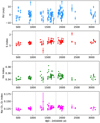 |
Fig. 1 From top to bottom: original RV (derived with the TERRA pipeline), S-index, Hα-index, and Na I D1, D2 -index time series for GJ 9689. Vertical dotted lines indicate the first three observing seasons as used in our study. |
5 Origin of the RV variations
5.1 Activity indexes
In order to disentangle the effects of activity in the measured RVs from other possible effects, we made use ofseveral spectroscopic indicators of chromospheric activity, the Ca II H and K (S-index), Hα, and Na I D1, D2 lines. Although these quantities are provided by the TERRA pipeline, the Hα, and Na I activity indexes came without uncertainty measurements. Therefore, we decided to measure the activity indexes following the definitions provided by Gomes da Silva et al. (2011, 2018).
Figure 1 shows the temporal variation of the different activity indexes, while the periodogram analysis is given in Fig. 4. A long-term activity trend in the three time series is seen. The trend has a period of ~34 500 d, 20 400 d, and 56 500 d in the S-index, Hα, and Na I index, respectively, suggesting an activity cycle of more than 55 yr4. We note that these periods are much longer than the observation timespan, so they are extremely uncertain. Once the long-term activity trend is subtracted by a sinusoidal fit, a group of peaks with periods in the range from 35–45 d is found in all the activity indexes. The highest peaks are located at 35.55 ± 0.05 d (S-index), 39.27 ± 0.03 d (Hα-index), and 42.54 ± 0.10 d (Na I-index). A clear peak close to the RV signal at 39.31 d is found in the three indexes.
Our analysis also shows that there is a peak close to 18.27 d in the S-index, although it is not significant. No significant peaks seem to be present at 18.27 days in either the Hα-index or in the Na I-index.
As an additional test, we checked whether our derived RVs show any correlation with the activity indexes finding no significant correlation between these quantities. The corresponding plots are shown in Fig. 5. For the S-index, the Spearman’s rank ρ is 0.1890 ± 0.0752 with a z-score = 1.058 ± 0.431; whereas for RVs and the Hα-index, we obtain ρ = 0.1214 ± 0.0772 and z-score = 0.675 ± 0.433. If the activity indexes are corrected by the long-term activity trend, we then obtain ρ = 0.2384 ± 0.0756 and z-score = 1.346 ± 0.4444 for the S-index, and ρ = 0.2283 ± 0.0756 and z-score = 1.286 ± 0.441 for the Hα-index. The statistical tests were performed by a bootstrap Monte Carlo simulation plus a Gaussian random shift of each data point within its error bars (Curran 2014)5.
Finally, we also computed the autocorrelation function (ACF) for the RVs, S-index, and Hα indexes. The corresponding plots are shown in Fig. B.2 (left). The ACF function was computed following the prescriptions given by Edelson & Krolik (1988), using a python wrapper developed by Robertson et al. (2015). It is clear that the three datasets show a periodicity around ~40 d. But the plot also shows that only in the RV data is there another periodicity at ~20 d. In order to confirm that, we also computed the GLS periodogram of the ACFs (Fig. B.2, right). While in the RV dataset the periods at ~18.27 and 39.31 d are clearly visible, the ACF function of the activity indicators only show the period at 39.31 d. We note that the ACF of the Hα index shows a peak around 17.3 d, but it is not statistically significant; indeed, there is a more significant period at ~11.8 d.
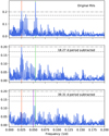 |
Fig. 2 Top: GLS periodogram of the TERRA RV measurements. Middle: GLS periodogram after subtracting the 18.27 d period. Bottom: GLS periodogram after subtracting the 18.27 and the 39.31 d signals. Values corresponding to a FAP of 10, 1, and 0.1% are shown with horizontal grey lines. The vertical red line indicates the period at 39.31 d, while the vertical green line shows the 18.27 d period. The first harmonic of the 39.31 d signal is shown in violet. |
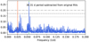 |
Fig. 3 GLS peridogram when the 39.31 d signal is subtracted from the original RV measurements. Values corresponding to a FAP of10, 1, and 0.1% are shown with horizontal grey lines. The vertical red line indicates the period at 39.31 d, while the vertical green line shows the 18.27 d period. |
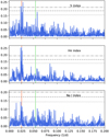 |
Fig. 4 From top to bottom: GLS periodogram of the S, Hα, and Na I activity indexes after the subtraction of the long-term activity trend. The vertical red line indicates the RV period at 39.31 d, while the vertical green line shows the RV period at 18.27 d. Values corresponding to a FAP of 10, 1, and 0.1% are shown with horizontal grey lines. |
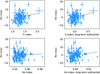 |
Fig. 5 Activity indexes versus RVs. Top left: S-index. Top right: S-index after the subtraction of the long-term activity trend. Bottom left: Hα-index. Bottom right: Hα-index after the subtraction of the long-term activity trend. The grey line shows the best linear fit. |
5.2 Periodogram power as a function of time
Another way to disentangle the variations of RVs due to the presence of planets from stellar activity is to study the evolution of the periodogram power of the RVs periods as a function of the number of observations (e.g. Affer et al. 2016; Mortier & Collier Cameron 2017). Activity regions change in shape and position with time, thus producing incoherent (in amplitude and phase) signals. In the periodograms, this incoherency translates into wider peaks and/or a bunch of peaks next to the central one. On the other hand, a Keplerian signal gains in power with time thanks to its coherency.
Figure 6 shows the variation in the periodogram power as a function of the number of observations for the periods found in the time series of RVs. For this exercise, we used the Bayesian generalised Lomb-Scargle periodogram (BGLS, Mortier et al. 2015) which computes the relative probability between peaks.
The analysis reveals that even at a relatively low number of observations, around 35–40, a period between 18 and 19 d is visible. At around ~110 observations, the period is well stabilised at ~18.27 d and since then, it remains constant in period and logPrb (Fig. 6, left).
The analysis also reveals a signal at a period slightly larger than 40 d, although at a rather modest probability; however, this signal disappears at around 30 observations. This signal is likely the previously identified ~39 d RV signal but not well constrained due to the low number of observations. A new period around 39 d appears again when the number of observations is around 80. The period of this signal is not well-constrained and it is worth noticing that it is accompanied by many other signals (Fig. 6, right).
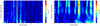 |
Fig. 6 Stacked-BGLS periodogram of the HARPS-N RV data of GJ 9689. Left: zoom around the 15–25 d region. Right: zoom around the 30–45 d region. |
5.3 Photometry
5.3.1 EXORAP photometry
GJ 9689 was observed photometrically within the EXORAP (EXOplanetary systems Robotic APT2 Photometry) programme from MJD =56 783 d to MJD = 58 034 d. Observations were carried out at the Serra la Nave observatory on Mount Etna (Italy) using a 80-cm f/8 Ritchey-Chretien robotic telescope (Automated Photoelectric Telescope, APT2). A total of 203, 201, 202, and 209 observations were obtained in the photometric bands B, V, R, and I, respectively. The corresponding light curves are shown in panels a–d in Fig. 7.
A search for periodicities reveals the presence of a long-term signal with periods of ~244 d (B), ~256 d (R), and ~270 d (I). No long-term trend is found in bandV. Once these long-term trends are subtracted, the corresponding GLS analysis (Fig. 8 panels a–d) reveals the presence of several signals with periods between ~35 and 39 days. The highest periods are found at 34.87 ± 0.15 d (B), 38.51 ± 0.16 d (V), 38.85 ± 0.16 d (R), and 34.97 ± 0.18 d (I). The significance of these peaks is better than 0.1% in bands B, V, and R, but slightly lower than 10% in band I. The periodograms of the Vand R bands (Fig. 8 panels b and c) also show some amount of power in the region around 18 days. However, no clear peaks are found at 18.27 days.
A comparison of Figs. 1 and 7 shows that the star is brighter when the activity S-index is lower. This behaviour is quite different from what we observe in the Sun (and similar stars), where long-term variability is dominated by faculae. We thus speculate that the stellar activity in GJ 9689 is spot-dominated (Radick et al. 2018).
5.3.2 APACHE photometry
The APACHE (A PAthway toward the Characterisation of Habitable Earths) photometric survey (Sozzetti et al. 2013) observed GJ 9689 with a 40-cm telescope located in the Astronomical Observatory of the Autonomous Region of the Aosta Valley. The observationscover a time span of 122 days from HJD = 2 456 445 d to HJD = 2 456 567 d. The number of observations amounts to 158. A Johnson I filter was used to carry out the observations. A clear significant period is found at 38.22 ± 1.04 d in the GLS analysis.
We note that APACHE and EXORAP I datasets have a different sampling, baselines, and data quality so it is not surprising to find slightly different periodograms. In particular, the EXORAP dataset covers a baseline of ~1250 d, allowing us to detect a long-term signal (~270 d) while the APACHE baseline is only 122 d.
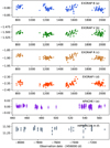 |
Fig. 7 Original photometry time series: (a) EXORAP B, (b) EXORAP V, (c) EXORAP R, (d) EXORAP I, (e) APACHE I, and (f) HIPPARCOS H. We note that the observations are not contemporaneous. For EXORAP, observation dates are in JD, for APACHE they are in HJD, while for HIPPARCOS observation dates are in BJD. |
5.3.3 Hipparcos H band photometry
We also analysed the available HIPPARCOS (ESA 1997) H band photometry. GJ 9689 was observed for 975 days between BJD = 2 447 964 d and BJD = 2 448 939 d, with a total of 101 data points. The corresponding periodogram is shown in panel f of Fig. 8, where no significant periods are found. While it is true that a peak seems to be present at ~18 d, it is very far from being significant. Furthermore, this region of the periodogram is largely crowded with numerous peaks with a similar (or larger) power.
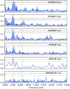 |
Fig. 8 GLS periodograms of the photometry datasets. Panels a, c and d: EXORAP B, R, and I band photometry after subtracting the corresponding long-term periods (see text for details). Panels b, e, f: original (i.e. no long-term period subtracted) EXORAP V, APACHE I, and HIPPARCOS H photometry analysis. Values corresponding to a FAP of 10, 1, and 0.1% are shown with horizontal grey lines. The vertical red line indicates the period at 39.31 d, while the vertical green line shows the 18.27 d period. |
5.4 Wavelength dependence
We also explored the dependence of the periodic signals identified in the RV analysis on the wavelength. In order to do that, we proceeded as in Tuomi et al. (2013) and exploited the fact that the TERRA pipeline allows us to select a blue cut-off aperture when computing the RVs. The results are shown in Fig. 9, which shows the GLS periodogram of the RVs obtained by using different blue cut-off wavelengths. It can be seen that the period at 18.27 days is always visible, independently of the bluest échelle aperture used in the computations of RVs. On the other hand, the period at 39.31 days disappears when only wavelengths redder than ~600 nm are used in the computations of RVs (two bottom panels).
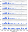 |
Fig. 9 GLS periodograms of the TERRA RVs as a function of the blue cut-off wavelength. From top to bottom: RVs were computed using the 1, 16, 22, 37, 55, and 61 aperture as a blue cut-off. Values corresponding to a FAP of 10, 1, and 0.1% are shown with horizontal grey lines. The vertical red line indicates the period at 39.31 d, while the green line shows the 18.27 d period. |
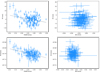 |
Fig. 10 CCF asymmetry diagnostics versus RV. Left: FWHM. Right: BIS. The grey line shows the best linear fit. Upper panels show the TERRA RVs, while bottom panels show the results for the DRS RVs. |
5.5 CCF asymmetry diagnostics
Stellar spotsand pulsations are known to affect the shapes and the centroids of the spectral lines. For possible correlations, we therefore investigated between the RVs and several CCF asymmetry diagnostics, namely the CCF width (FWHM) and its bisector velocity span (BIS; e.g. Queloz et al. 2001, 2009; Boisse et al. 2009). Both quantities are directly provided by the HARPS-N DRS. As mentioned before, these quantities should be taken with caution when dealing with low-mass stars. Figure 10 (upper panels) shows the TERRA RVs as a function of the FWHM and BIS values. A Spearman’s correlation test confirms that there is no monotone dependence between the RVs and the measured FWHM values (ρ = −0.1304 ± 0.0807 and z-score = −0.726 ± 0.454) or between the RVs and the BIS (ρ = 0.0315 ± 0.0781 and z-score = 0.174 ± 0.433). Furthermore, no significant signals were found in the periodogram analysis of the BIS. For the FWHM, a rather broad but statically significant period is found at ~402 ± 8 d, but no significant periods remain after this period is pre-whitened. No signals are found either in BIS or in FWHM around the periods identified in the RV analysis.
Given that TERRA RVs are derived using a different method (and a different pipeline), a comparison between the FWHM and BIS values with the RVs derived by the CCF performed by the HARPS-N DRS is also mandatory. The corresponding plots are shown in Fig. 10 (bottom panels). We find that the results are similar to the ones obtained using the TERRA RVs, that is, there is no dependence between the DRS RVs and the measured FWHM or BIS values (ρ = −0.2990 ± 0.0732 and z-score = −1.712 ± 0.446 for the FWHM, and ρ = −0.0087 ± 0.0797 and z-score = −0.048 ± 0.443 for the case of the BIS).
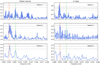 |
Fig. 11 GLS periodograms for the different seasons analysed. Left: RVs. Right: S-index. Values corresponding to a FAP of 10, 1, and 0.1% are shown with horizontal grey lines. The vertical red line indicates the period at 39.31 d, while the vertical green line shows the 18.27 d period. |
5.6 Analysis of individual seasons
In this section we analyse the data by considering three different observing seasons. They are indicated with vertical lines in Fig. 1. We note that ‘season 1’ and ‘season 2’ do indeed contain data from two observing seasons. This choice was made in order to have enough RV data points in each season. The first season includes 46 data points taken from May 26, 2013 to October 22, 2014. The second season covers the observations performed between August 23, 2015 and November 28, 2016 with 62 observations. Finally, we consider 47 observations between April 16, and October 10, 2017. The remaining observations are not considered as they are sparse in time and amount only to 19.
The RV and S-index periodogram for each season are shown in Fig. 11 (left and right, respectively). The vertical red and green line indicate the identified periods at 39.31 d and 18.27 d, respectively. The figure clearly shows that the RV period at 18.27 d is visible in all seasons, with a similar structure and power. However, the structure of the RV period at 39.31 d changes from one season to another. The peak is located at 38.53 d, 39.25 d, and 35.93 d in the first, second, and third season, respectively. Its power also changes with time, being the dominant signal in the second and third seasons. We note that in these seasons, the values of the S-index are higher than in the first season (see Fig. 1), supporting the hypothesis that the ~39.31 d period is due to stellar activity. Regarding the S-index (right panel), there are no signals close to 18.27 d in any of the seasons, while there are prominent signals close to 39.31 d in all seasons. The structure of these signals change from one season to another and the highest periods are located at 42.56 d, 40.76 d, and ~178 d in the first, second, and third season, respectively.
5.7 Spectral window analysis
Given that the periods found in the RV time series of GJ 9689 are at 18.27 d and 39.31 d, it is reasonable to ask whether the signal at 18.27 d is the first harmonic of the signal at 39.31 d. To answer this question, Fig. 12 (top panel) shows the spectral window of the original RV dataset of GJ 9689. There are three prominent peaks at frequencies of 0.000854 d-1, 0.001895 d-1, and 0.002749 d-1. These peaksare related to the gaps in the RV curve (Fig. 1). There is the obvious 1 cycle/year peak (0.00275 d-1) and two peaks related to the poor sampling in the 2 458 000–2 459 100 BJD interval: 1 cycle/1100 d (0.0009 d-1) and 1 cycle/550 d (0.0018 d-1). The presence of a peak in the spectral window at 0.001895 d-1 might indicate an alias phenomenon as 0.001895 d-1 + 0.025436 d-1 (frequency of the 39.31 d period) is 0.027331 d-1, which is close to 0.054734/2 d-1 (≈0.027367 d-1, i.e. half the frequency of the 18.27 d period).
To further investigate this possibility, we also analysed the spectral window in the three different seasons previously considered. The results are shown in Fig. 12 where for each season we indicate, with a magenta line, the position that a peak in the spectral window should have in order to produce the aliasing phenomenon between the39.31 d and 18.27 d periods. The analysis takes into account that the signals appear at slightly different frequencies in the different seasons. For example, in season one, the 39.31 d signal appears at 38.53 d (f = 0.025953 d-1), while the 18.27 d signal is at 18.24 d (f= 0.045823 d-1). If the 38.53 d and 18.27 d were related by an alias phenomenon due to a signal in the window function, this signal should appear at a frequency offwin ≈ 0.001458 d-1. As it can be seen in Fig. 12 (second panel from top), there is no such signal in the window function of season one. The same happens in the second season (third panel from the top). In this case, the 39.31 d signal appears at 39.24 d (f = 0.02548 d-1) and the 18.27 d at 18.14 d (f = 0.055122 d-1). If the signal at 18.14 d were an alias of the 39.24 d signal, there should be a signal in the window function at a frequency of fwin ≈ 0.0021 d-1, which is not the case. In the third season (bottom panel), the signals are located at 35.93 d (f = 0.027835 d-1) and 18.71 d (f = 0.053457 d-1). Again, thereare no peaks in the spectral window that might originate from an aliasing phenomena. We conclude that it is unlikely that the 18.27 d signal is the harmonic of the 39.31 d, a result which is in line with all the different analyses performed before.
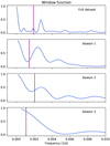 |
Fig. 12 Spectral window when the full RV dataset is considered (top) and for each of the different analysed seasons. The magenta line indicates the frequency that a signal in the spectral window should have in order to produce an aliasing phenomenon between the ~18.27 d and ~39.31 d periods. |
6 Modelling the RV variations
The analysis performed in the previous section is consistent with a Keplerian origin of the coherent signal at 18.27 d, while the incoherent signal at 39.31 d seems to be related to the rotation period of the star. This conclusion is based on the following observational facts:
Firstly, a periodicity close to 39.31 d is found in the analysis of the main optical activity indicators as well as in the analysis of the available photometry. Secondly, its power and frequency changes with the number of observations and from one observing season to another. Finally, this signal tends to disappear if only the reddest region of the spectra is used for the computation of the RVs.
On the other hand, for the 18.27 period: it does not seem to be related (to be a harmonic) of the 39.31 days period. No hint of this period is found in the activity indexes, photometry, or CCF asymmetry indicators. It appears in all observing seasons at a similar frequency and similar power. In addition, it does not show variations as a function of the number of observations. Finally, it is always found in the RVs analysis even if only the reddest region of the spectra is considered.
In order to model the RV data, we have defined a Bayesian framework based on a Monte Carlo sampling of the parameter space with a Gaussian process (GP) model. Before modelling, a 3σ clipping algorithm was applied to the RVs to identify potential outliers that might affect the results. As a consequence, two data points were excluded from the following analysis. The likelihood function is given by
 (1)
(1)
where yn, tn, and σn are the RVs, time of observations, and errors, respectively; θ is the array of parameters; r is the residual vector obtained by removing the (deterministic) model from data; K is the covariance matrix; and N is the number of observations.
The covariance (or kernel) function adopted in this analysis is a quasi-periodic (QP) function and it was obtained by multiplying an exp-sin-squared kernel to a squared-exponential kernel (george python package, Ambikasaran et al. 2015) added to an extra white noise (jitter) term, and it is defined as follows
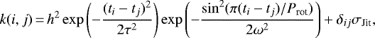 (2)
(2)
where k(i, j) is the ij element of the covariance matrix, ti and tj are two times from the RV dataset, h is the amplitude of the covariance, τ is the timescale of the exponential component, ω is the weight of the periodic component, Prot is the period, δij is the Kronecker delta function, and σJit is the white noise term.
The parameter space was sampled with emcee (Foreman-Mackey et al. 2013), based on the affine-invariant ensemble sampler for Markov chain Monte Carlo (MCMC; Goodman & Weare 2010). In this analysis we have compared two models which differ as to whether there is a presence of a planetary (Keplerian) signal (Fulton et al. 2018), but they share the effect of a linear trend (characterised by the parameters γ and  ), being ‘GP-only’ and ‘star-planet’ models, respectively.
Priors of the models are reported in Table 2, they have been chosen to be uninformative and as large as possible. This parameter space is covered by 32 walkers, randomly initialised within the priors ranges. This choice on the initial position of the walkers produces very low probability values at the beginning of the emcee chain. These values were eliminated by a burn-in phase, here it was set as the first 20 K steps. After the burn-in phase, a blob, centred at the maximum probability position, was initialised to feed a following chain. This chain ran until the autocorrelation time of each parameter (see Sokal 1997), evaluated every 10 K steps, varied less than 1% and the chain was 100 times longer than the estimated autocorrelation time. With this definition of convergence, chains converged after 120 and 270 K steps for the GP-only and star-planet models, respectively.
The resulting posterior distributions are presented in Figs. 13 and 14, respectively. As an estimate of the goodness of the model, we calculated the Bayesian information criterion (BIC), which is defined as follows
 (3)
(3)
where k is the number of model parameters, N is the number of data points, and  is the maximum likelihood of the model. We obtain that there is strong evidence in supporting the star-planet model (BIC = 912.4) against the GP-only model (BIC = 930.9) because the BIC difference is more than 10 (Kass & Raftery 1995). Figure 15 shows the best-fit star-planet model (top), the corresponding RV residuals (middle), and the RV curve folded at the best-fit orbital period for the detected planet (bottom). The best-fit parameters are listed in Table 2. Given that the derived eccentricity is not statistically significant, we also provide the 68% upper limit. We attempted a star-planet model with zero eccentricity finding that the corresponding BIC value is almost identical to the eccentric model.
In order to test whether the GP part of the model can generate a spurious signal at ~18 d, we derived a FAP-like significance of the ~18 d signal by drawing a sample of 104 RV curves from the star-planet model using the best fit parameters but excluding the planetary part. Then, we counted how many samples have the power of the ~18.27 d signal greater than the value obtained by evaluating the periodogram on the original RV data. This condition was never achieved.
As a further investigation, we also checked on the stability of the planetary signal by applying the same GP analysis with the star-planet model to the seasons defined in Sect. 5.6. In this case, we set the burn-in phase to 50 K steps and we ran the second chain until it reached 100 K steps.
Due to the small number of points in each season, we shortened the prior ranges of the kernel and the linear trend parameters within 1σ from the median of the posterior distributions presented in Fig. 14. For the same reason, the orbital period was constrained within 3σ while the other prior ranges remained unchanged with respect to the previous analysis. The result of this analysis is presented in Table 3. We note that in all seasons, we derived the same planetary parameters (within the uncertainties) which shows that the Keplerian signal is coherent in all seasons.
As an additional test on the stability of the planetary signal, we analysed how the RV semi-amplitude varies as a function of the number of observations. The results are shown in Fig. 16 where it can be seen that starting from ~85 observations, the value of Kb remains constant within the uncertainties around a value of 3.5 ms-1. We note that for this exercise, we ran the star-planet model with the priors as listed in Table 2 and ran the second chain until it reached 100 K steps.
For the sake of completeness, we tested a model with a second additional planet. Given that the RV time-series analysis reveals no more addition signals to the ones already discussed, we performed a blind search, using a wide prior for the period of the second planet. More specifically, we tested a model with a second planet with a period between 1 d and 100 d, between 100 d and 200 d, and between 200 d and 300 d. None of these models provide a lower BIC than the ‘one planet - star’ model, confirming that, if there are more planets in the system, they are difficult to reveal with the data at hand.
We also ran the star-planet model using the quasi-periodic with cosine (QPC) kernel defined in Perger et al. (2021). The QPC kernel is defined as a QP kernel, but it adds an additional term in order to account for the Prot/2 peaks in theautocorrelation function. The corresponding results are given in Table 3. It can be seen that the best obtained values are almost identical to the ones derived using the QP. The QPC has a BIC value of 917.6, which is slightly larger than the value obtained using the QP kernel (BIC = 912.4).
As a final test, we also explored the full (hyper)-parameter space using the publicly available Monte Carlo (MC) nested sampler and Bayesian inference tool MULTINEST V3.10 (e.g. Feroz et al. 2019), through the PYMULTINEST wrapper (Buchner et al. 2014). MULTINEST is known to provide accurate estimates of the Bayesian evidence  , which can be used to perform a statistical comparison between different models. To test the planetary nature of the ~18 day signal (circular orbital approximation), we fitted the RVs using two different GP models. For the first model, we adopted only a QPC kernel, while the second model is represented by the combination of a QP kernel and a sinusoid. For the hyper-parameter representingthe stellar rotation period, which is the same both in the QPC and QP GP kernels, we used the uninformative prior
  (20, 50) days. Both models are assumed to have an equal a priori likelihood. As in our previous analyses, we found that the QP plus planetary model is strongly favoured over the GP-only QPC model (
 = +7.3, corresponding to an odds ratio of ~1500:1), following the convention usually adopted for model selection (e.g. Feroz et al. 2011, Table 1). This result shows that the ~18 day signal is much better fitted by a sinusoid, rather than being modelled through a QPC kernel as the first harmonic of the stellar rotation period.
Best-fit values obtained for the star-planet model.
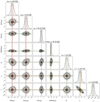 |
Fig. 13 Posterior distribution of the GP-only model in which median and maximum a-posterior probability (MAP) have been marked (respectively, red and green line). |
7 Discussion
From the best values of Kb and Pb derived in the previous section, we derived a minimum mass for GJ 9689 b of MP sini = 9.65 ± 1.41 M⊕ and a semi-major axis a = 0.1139 ± 0.0039 au (for the formulae see e.g. Cumming et al. 1999, Eqs. (1) and (3)). GJ 9689 b is therefore a super-Earth or a mini-Neptune-like planet. Figure 17 shows the position of GJ 9689 b in the planetary mass versus period diagram. For comparison purposes, the location of the known (RV) planets around M dwarf stars are shown. It can be seen that GJ 9689 b has a period and a minimum mass similar to other HADES planets. We note that most of the HADES discoveries have periods shorter than 20 d and minimum masses lower than the mass of Neptune. Only one HADES planet, namely GJ 15 Ac, has a higher mass and an orbit at a wide distance from its host star, P ~ 7600 d (Pinamonti et al. 2018). This is in agreement with other RV surveys that found that the frequency of gas-giant planets around M stars is lower than that around solar-type hosts (Endl et al. 2003, 2006; Butler et al. 2006; Bonfils et al. 2007; Cumming et al. 2008; Johnson et al. 2010).
Following the definition of the habitable zone (HZ) of Kopparapu et al. (2013), the inner edge of the HZ for GJ 9689 was computed with the most optimistic limits (recent Venus), corresponding to a semi-major axis of aHZ = 0.20 au, which is larger than the orbit of GJ 9689 b. The equilibrium temperature of the planet can be determined from the balance between the incident radiation from the host star and that absorbed by the planet (or by its atmosphere). It can be written as:
![\begin{equation*}T_{\textrm{eq}}\,{=}\,T_{\star}\left(\frac{R_{\star}}{2a}\right)^{1/2}\left[f\left(1-A_{\textrm{B}}\right)\right]^{1/4},\end{equation*}](/articles/aa/full_html/2021/07/aa41141-21/aa41141-21-eq9.png) (4)
(4)
where additional heat sources (such as the greenhouse effect) are not taken into account. In this equation, AB is the Bond albedo and f is the heat redistribution factor. The value of f goes from f = 1 for an isotropic planetary emission to f = 2, when only the day-side re-radiates the energy absorbed, as it could be the case for tidally locked planets without oceans or an atmosphere (Charbonneau et al. 2005; Méndez & Rivera-Valentín 2017). An upper limit on Teq may be obtained by setting AB = 0. For GJ 9689 b, we find upper limits on Teq between 413.88 K (f = 1) and 492.19 K (f = 2). Therefore, GJ 9689 b has a Teq which is ~140–240 K higher than the equilibrium temperature of the rocky planets in our Solar System. For example Venus has Teq ~ 230 K, while the Earth has a value of ~255 K, and for Mars we have Teq ~ 212 K (Perryman 2018). However, the equilibrium temperature of GJ 9689 b is in agreement with the values derived for other super-Earth planets found around M dwarfs, such as GJ 3998 c, ~420 K, or Gl 886 b, ~379–450 K (Affer et al. 2016, 2019).
The composition of exoplanets is an important, but highly problematic issue. To start with, error uncertainties in stellar radius and mass are usually large and lower values of mass and radius for the host star translate to overall higher densities (e.g. Modirrousta-Galian et al. 2020). Even if the planet transits, and accurate planetary mass and radius measurements are available, the composition of low-mass planets is plagued with degeneracies that mainly arise from trade-offs between thedifferent composition building blocks (e.g. Valencia et al. 2007; Rogers & Seager 2010; Plotnykov & Valencia 2020).
In order to solve this problem, several works have suggested using the abundances of refractory elements of the host star to constrain the refractory content of the planet, which is likely a good approximation from a statistical approach (e.g. Dorn et al. 2015; Brugger et al. 2017; Santos et al. 2017). Recently, Maldonado et al. (2020) determined the stellar abundances of a large sample of M dwarfs for several elements other than iron analysing high-resolution optical spectra. Using these abundances,we estimated the core mass fraction (CMF) of 52 rocky exoplanets (planetary masses between 1 and 20 M⊕) around M dwarfs. We followed the CMF definition as provided in Schulze et al. (2021) that assumes that the planetary core is pure iron and that the mantle reflects fully oxidised Mg and Si. The results are shown in Fig. 18 where the histogram of the derived CMFs is shown. We find that the CMF values of small planets around M dwarfs varies from 0.27 to 0.52 with a median value of 0.38. According to our results, GJ 9689 b has a CMF value 0.34, close to the median of the distribution. It is worth noticing that these values are slightly larger than the CMF values derived for 11 transiting planets around FGK stars (median CMF = 0.29) in Schulze et al. (2021). This trend, if confirmed, may indicate that small planets around M dwarfs might have larger cores.
Finally, we should note that the derived timescale of active regions is shorter in the GP-only model than in the star-planet model. While the former, τGP = 64.57 d, is consistent with roughly two rotation periods, the latter, τGP = 157.84
 d, is much larger (around 4.0 rotation periods) and consistent with the typical active region lifetimes derived for other M dwarf stars (Scandariato et al. 2017; Pinamonti et al. 2019). To further investigate this issue, we ran our GP-only model for the S-index time series and the V band EXORAP photometry, although the results did not allow us to reach a clear conclusion. Results for the S-index provide a typical active regions timescale of τGP = 63.87
 d, although the distribution is rather broad and has a tail towards larger values. However, the analysis of the V band photometry returns a correlation decay timescale of τGP = 38.27
 d, which is comparable to the stellar rotation period, but a secondary peak appears at τGP ~100 d. The corresponding corner plots can be seen in Fig. B.3 (S-index fit) and in Fig. B.4 (EXORAP photometry).
GJ 9689 is expected to be observed by the Tess mission (Ricker et al. 2015) in 2022 in Sector 54 (July 9 to August 5, in cycle 4). In order to get an estimate of the transit probability and depth for GJ 9689 b, a value of the planetary radius is needed. Using the probabilistic mass-radius relationship by Chen & Kipping (2017), we obtain a radius of RP = 2.92 R⊕ for GJ 9689 b which implies a geometric transit probability of 2.5% and a transit depth of 0.23%. Although the transit probability is rather low, a potential transit might provide a constraining point in the mass-radius diagram of known planets and also enable one to determine the bulk density. A comparison of the CMF derived by assuming that the planet reflects the host star’s major rocky building elemental abundances and the CMF value derived from the planetary bulk density might help us to unravel how GJ 9689 b formed and evolved.
Astrometric measurements are another source of information that might be used for the characterisation of the GJ 9689 planetary architecture. Gaia EDR3 data (Gaia Collaboration 2020) show that GJ 9689 has an astrometric noise of 73 μas (with a statistical significance of 6.5σ) and a re-normalised unit weight error (RUWE) value of 0.996. Furthermore, no significant proper motion anomaly between Gaia DR2 and Hipparcos has been reported (Kervella et al. 2019). Therefore, it is plausible that there are no massive companions at long periods. Detailed RV detection limits for the stars observed within the framework of the HADES survey will be addressed in a forthcoming work.
It is worth noticing that GJ 9689 b is not the first planet around an M dwarf with an orbital period close to half the stellar rotation period. Some examples include Gl 49 b (Perger et al. 2019) or GJ 720 Ab (González-Álvarez et al. 2021). The detection of such planets is challenging. It is known that dark spots in the stellar surface might produce a RV modulation with a period of Prot/2, while the induced RV period due to the suppression of the surface convection is equal to Prot (see e.g. Lanza et al. 2010). The period found in the RV might be slightly different from Prot/2 due to several phenomena such as differential rotation or the evolution of the spot in the active longitude. While lifetimes of active longitudes are not well known, the possibility of an active longitude with time scales of several years might not be excluded in M dwarfs. We note that single spots may survive even for hundreds of days in the surface of M dwarfs (e.g. Giles et al. 2017). In the case of GJ 9689, given its rotational period and the photometric variability of the star, and assuming a stable active longitude covered by dark spots with an area of 1% of the stellar disc, we derived a semi-amplitude of ~7.2 ms-1 for the signal due to the magnetic activity of such spots, which is larger than the observed RV variability.
This consideration and all the analysis performed in this work make us confident that the signal at 18.27 d found in the RV time series of GJ 9689 is truly Keplerian in nature. An ‘ultimate’ confirmation of planets such as GJ 9689 b will likely be possible in the near future if high-resolution spectrographs in the near-infrared domain are able to reach enough RV precision.
Best-fit values obtained for the star-planet model when using the full dataset of RVs, and the data corresponding to the different seasons analysed in this work.
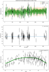 |
Fig. 15 Best-fit star-planet model (top), RV residuals (middle), and RV curve folded at the best-fit orbital period for GJ 9689 b (bottom). |
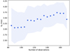 |
Fig. 16 RV semi-amplitude derived for GJ 9689 b using the star-planet model described in the text as a function of the number of observations. The shadow region indicates the 1σ uncertainties. |
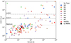 |
Fig. 17 Known RV planets (planetary mass versus orbital period diagram) around M dwarfs (As listed at http://exoplanet.eu/ in December 2020). Planets discovered by the HADES survey are shown as red triangles. The planet GJ 9689 b is shown as a black star. |
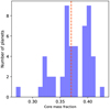 |
Fig. 18 Histogram of derived CMF for suspected rocky planets around M dwarfs. The vertical red line shows the median of the distribution. |
8 Conclusions
Understanding the origin and evolution of stars and planetary systems is one of the major goals in modern astrophysics. M dwarfs have emerged as promising targets in the search for small planets. Being less massive and cooler than solar-type stars, planets have a larger RV amplitude and their habitable zones are closer to the host star (e.g. Reiners et al. 2010). However, the expected periods of planets in the habitable zone around M stars may be comparable to the rotation period of the host star. As a consequence, unravelling the origin (stellar or truly Keplerian) of periodic signals in the RV dataset of M dwarfs is a complicated task.
The nearby M dwarf GJ 9689 is an example of this problematic. In this workwe have analysed more than seven years of RV data points of GJ 9689. The RV analysis reveals two signals at 39.31 d and 18.21 d. A detailed study of the main activity indexes and photometry allows us to identify the 39.31 d as the rotation period of the star. This hypothesis is confirmed by studying the stability of this signal as a function of the number of observations, epoch of observations, and spectral range used to compute the RV.
A careful analysis of the spectral window in several observing seasons shows that the 18.27 d signal is not a harmonic or an alias of the 39.32 d period. In addition, activity indexes, CCF asymmetry indicators, and photometric data show no variability at all at 18.27 d. The signal is stable in all analysed epochs, it does not show variations with the number of observations, and it is also visible even if only the reddest part of the spectra are used in the computation of the RV dataset. We therefore conclude that the 18.27 d signal is most likely truly Keplerian in nature. In order to derive the minimum mass and orbital parameters of GJ 9689 b, we fitted the RV time series with a Keplerian model combined with a GP quasi-periodic model to take the stellar activity signal into account. We obtain a period of P = 18.27 ± 0.01 d, a semi-major axis of a = 0.114 ± 0.004 au, and a minimum mass of MP sini = 9.65 ± 1.41 M⊕. Assuming that the composition of a rocky planet directly mirrors the relative Fe, Mg, and Si abundances of its host, we derived the CMF of several suspected rocky planets around M dwarfs, finding that the CMF value of GJ 9689 b is close to the median value of the distribution.
GJ 9689 b joins the population of super-Earths at short periods (P < 20 d) around M dwarfs that is currently emerging (see Fig. 17). Further studies of the properties of these planets will help us to explore a regime of protoplanetary disc and host star conditions that are very different from FGK stars, providing additional constraints for planet formation models.
Acknowledgements
J.M. and G.M. acknowledge support from the accordo attuativo ASI-INAF n.2021-5-HH.0 “Partecipazione italiana alla fase B2/C della missione Ariel”. A.P., A.M., M.P., and A.S. acknowledge partial contribution from the agreement ASI-INAF n.2018-16-HH.0. E.G.A. acknowledges support from the Spanish Ministery for Science, Innovation, and Universities through projects AYA-2016-79425-C3-1/2/3-P, AYA2015-69350-C3-2-P, ESP2017-87676-C5-2- R, ESP2017-87143-R. The Centro de Astrobiología (CAB, CSIC-INTA) is a Center of Excellence “Maria de Maeztu”. M.P and I.R acknowledgesupport from the Spanish Ministry of Science and Innovation and the European Regional Development Fund through grant PGC2018-098153-B- C33, as well as the support of the Generalitat de Catalunya/CERCA programme. J.I.G.H. acknowledges financial support from Spanish Ministry of Science and Innovation (MICINN) under the 2013 Ramón y Cajal program RYC-2013- 14875. B.T.P. acknowledges Fundación La Caixa for the financial support received in the form of a Ph.D. contract. A.S.M. acknowledges financial support from the Spanish MICINN under the 2019 Juan de la Cierva Programme. B.T.P., A.S.M., J.I.G.H., R.R. acknowledge financial support from the Spanish MICINN AYA2017-86389-P. This work has made use of data from the European Space Agency (ESA) mission Gaia (https://www.cosmos.esa.int/gaia), processed by the Gaia Data Processing and Analysis Consortium (DPAC, https://www.cosmos.esa.int/web/gaia/dpac/consortium). Funding for the DPAC has been provided by national institutions, in particular the institutions participating in the Gaia Multilateral Agreement.
Appendix A Additional tables
Table A.1 (available at the CDS) provides the observational data collected with the HARPS-N spectrograph for GJ 9689 and used in the present study. We list the observations dates (in barycentric Julian date or BJD), the RVs, and activity S, Hα, and Na I D1, D2 indexes with their corresponding uncertainties.
Appendix B Additional figures
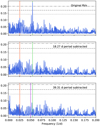 |
Fig. B.1 Top: GLS periodogram of the DRS RV measurements. Middle: GLS periodogram after subtracting the 18.27 d period. Bottom: GLS periodogram after subtracting the 18.27 and the 39.31 d signals. Values corresponding to a FAP of 10, 1, and 0.1% are shown with horizontal grey lines. The vertical red line indicates the period at 39.31 d, while the vertical green line shows the 18.27 d period. The first harmonic of the 39.31 d signal is shown in violet. |
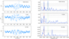 |
Fig. B.2 Left: autocorrelation function of RV, S-index, and Hα time series. Right: corresponding GLS diagrams. |
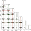 |
Fig. B.3 Posterior distribution of the GP-only model of the S-index time series in which median and maximum a-posterior probability (MAP) have been marked (respectively, red and green line). |
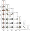 |
Fig. B.4 Posterior distribution of the GP-only model of the EXORAP V band photometry in which median and maximum a-posterior probability (MAP) have been marked (respectively, red and green line). |
References
- Affer, L., Micela, G., Damasso, M., et al. 2016, A&A, 593, A117 [NASA ADS] [CrossRef] [EDP Sciences] [Google Scholar]
- Affer, L., Damasso, M., Micela, G., et al. 2019, A&A, 622, A193 [NASA ADS] [CrossRef] [EDP Sciences] [Google Scholar]
- Ambikasaran, S., Foreman-Mackey, D., Greengard, L., Hogg, D. W., & O’Neil, M. 2015, IEEE Transactions on Pattern Analysis and Machine Intelligence, 38, 252 [Google Scholar]
- Anglada-Escudé, G., & Butler, R. P. 2012, ApJS, 200, 15 [NASA ADS] [CrossRef] [Google Scholar]
- Baranne, A., Queloz, D., Mayor, M., et al. 1996, A&AS, 119, 373 [NASA ADS] [CrossRef] [EDP Sciences] [Google Scholar]
- Bensby, T., Feltzing, S., & Lundström, I. 2003, A&A, 410, 527 [NASA ADS] [CrossRef] [EDP Sciences] [Google Scholar]
- Bensby, T., Feltzing, S., Lundström, I., & Ilyin, I. 2005, A&A, 433, 185 [NASA ADS] [CrossRef] [EDP Sciences] [Google Scholar]
- Boisse, I., Moutou, C., Vidal-Madjar, A., et al. 2009, A&A, 495, 959 [NASA ADS] [CrossRef] [EDP Sciences] [Google Scholar]
- Bonfils, X., Delfosse, X., Udry, S., et al. 2013, A&A, 549, A109 [NASA ADS] [CrossRef] [EDP Sciences] [Google Scholar]
- Bonfils, X., Mayor, M., Delfosse, X., et al. 2007, A&A, 474, 293 [NASA ADS] [CrossRef] [EDP Sciences] [Google Scholar]
- Brugger, B., Mousis, O., Deleuil, M., & Deschamps, F. 2017, ApJ, 850, 93 [Google Scholar]
- Buchner, J., Georgakakis, A., Nandra, K., et al. 2014, A&A, 564, A125 [NASA ADS] [CrossRef] [EDP Sciences] [Google Scholar]
- Butler, R. P., Johnson, J. A., Marcy, G. W., et al. 2006, PASP, 118, 1685 [NASA ADS] [CrossRef] [Google Scholar]
- Chabrier, G., & Baraffe, I. 2000, ARA&A, 38, 337 [NASA ADS] [CrossRef] [Google Scholar]
- Charbonneau, D., Allen, L. E., Megeath, S. T., et al. 2005, ApJ, 626, 523 [NASA ADS] [CrossRef] [Google Scholar]
- Chen, J., & Kipping, D. 2017, ApJ, 834, 17 [Google Scholar]
- Courcol, B., Bouchy, F., & Deleuil, M. 2016, MNRAS, 461, 1841 [NASA ADS] [CrossRef] [Google Scholar]
- Cumming, A. 2010, Statistical Distribution of Exoplanets, ed. S. Seager (Tucson, AZ: University of Arizona Press), 191 [Google Scholar]
- Cumming, A., Marcy, G. W., & Butler, R. P. 1999, ApJ, 526, 890 [NASA ADS] [CrossRef] [Google Scholar]
- Cumming, A., Butler, R. P., Marcy, G. W., et al. 2008, PASP, 120, 531 [CrossRef] [Google Scholar]
- Curran, P. A. 2014, ArXiv e-prints [arXiv:1411.3816] [Google Scholar]
- Cutri, R. M., Skrutskie, M. F., van Dyk, S., et al. 2003, VizieR Online Data Catalog: II/2246 [Google Scholar]
- Desort, M., Lagrange, A.-M., Galland, F., Udry, S., & Mayor, M. 2007, A&A, 473, 983 [NASA ADS] [CrossRef] [EDP Sciences] [Google Scholar]
- Dorn, C., Khan, A., Heng, K., et al. 2015, A&A, 577, A83 [EDP Sciences] [Google Scholar]
- Dressing, C. D., & Charbonneau, D. 2013, ApJ, 767, 95 [NASA ADS] [CrossRef] [Google Scholar]
- Dressing, C. D., & Charbonneau, D. 2015, ApJ, 807, 45 [NASA ADS] [CrossRef] [Google Scholar]
- Dumusque, X., Santos, N. C., Udry, S., Lovis, C., & Bonfils, X. 2011a, A&A, 527, A82 [NASA ADS] [CrossRef] [EDP Sciences] [Google Scholar]
- Dumusque, X., Udry, S., Lovis, C., Santos, N. C., & Monteiro, M. J. P. F. G. 2011b, A&A, 525, A140 [NASA ADS] [CrossRef] [EDP Sciences] [Google Scholar]
- Dumusque, X., Borsa, F., Damasso, M., et al. 2017, A&A, 598, A133 [NASA ADS] [CrossRef] [EDP Sciences] [Google Scholar]
- Edelson, R. A., & Krolik, J. H. 1988, ApJ, 333, 646 [NASA ADS] [CrossRef] [Google Scholar]
- Endl, M., Kürster, M., Els, S., Hatzes, A. P., & Cochran, W. D. 2001, A&A, 374, 675 [NASA ADS] [CrossRef] [EDP Sciences] [Google Scholar]
- Endl, M., Cochran, W. D., Tull, R. G., & MacQueen, P. J. 2003, AJ, 126, 3099 [Google Scholar]
- Endl, M., Cochran, W. D., Kürster, M., et al. 2006, ApJ, 649, 436 [Google Scholar]
- ESA, ed. 1997, The HIPPARCOS and TYCHO Catalogues. Astrometric and Photometric Star Catalogues Derived from the ESA HIPPARCOS Space Astrometry Mission (Noordwijk, The Netherlands: ESA Publication), 1200 [Google Scholar]
- Feliz, D. L., Plavchan, P., Bianco, S. N., et al. 2021, AJ, 161, 247 [Google Scholar]
- Feroz, F., Balan, S. T., & Hobson, M. P. 2011, MNRAS, 415, 3462 [Google Scholar]
- Feroz, F., Hobson, M. P., Cameron, E., & Pettitt, A. N. 2019, Open J. Astrophys., 2, 10 [Google Scholar]
- Foreman-Mackey, D., Hogg, D. W., Lang, D., & Goodman, J. 2013, PASP, 125, 306 [Google Scholar]
- Fulton, B. J., Petigura, E. A., Blunt, S., & Sinukoff, E. 2018, PASP, 130, 044504 [NASA ADS] [CrossRef] [Google Scholar]
- Gaia Collaboration 2020, VizieR Online Data Catalog: I/350 [Google Scholar]
- Giles, H. A. C., Collier Cameron, A., & Haywood, R. D. 2017, MNRAS, 472, 1618 [Google Scholar]
- Gillon, M., Triaud, A. H. M. J., Fortney, J. J., et al. 2012, A&A, 542, A4 [NASA ADS] [CrossRef] [EDP Sciences] [Google Scholar]
- Gomes da Silva, J., Santos, N. C., Bonfils, X., et al. 2011, A&A, 534, A30 [NASA ADS] [CrossRef] [EDP Sciences] [Google Scholar]
- Gomes da Silva, J., Figueira, P., Santos, N., & Faria, J. 2018, J. Open Source Softw., 3, 667 [Google Scholar]
- González-Álvarez, E., Micela, G., Maldonado, J., et al. 2019, A&A, 624, A27 [NASA ADS] [CrossRef] [EDP Sciences] [Google Scholar]
- González-Álvarez, E., Petralia, A., Micela, G., et al. 2021, 649, A157 [Google Scholar]
- Goodman, J., & Weare, J. 2010, Commun. Appl. Math. Comput. Sci., 5, 65 [Google Scholar]
- Hobson, M. J., Delfosse, X., Astudillo-Defru, N., et al. 2019, A&A, 625, A18 [NASA ADS] [CrossRef] [EDP Sciences] [Google Scholar]
- Howard, A. W. 2013, Science, 340, 572 [NASA ADS] [CrossRef] [PubMed] [Google Scholar]
- Howard, A. W., Marcy, G. W., Bryson, S. T., et al. 2012, ApJS, 201, 15 [Google Scholar]
- Johnson, J. A., & Apps, K. 2009, ApJ, 699, 933 [NASA ADS] [CrossRef] [Google Scholar]
- Johnson, J. A., Howard, A. W., Marcy, G. W., et al. 2010, PASP, 122, 149 [NASA ADS] [Google Scholar]
- Kass, R. E., & Raftery, A. E. 1995, J. Am. Stat. Assoc., 90, 773 [CrossRef] [Google Scholar]
- Kervella, P., Arenou, F., Mignard, F., & Thévenin, F. 2019, A&A, 623, A72 [NASA ADS] [CrossRef] [EDP Sciences] [Google Scholar]
- Klein, B., Donati, J.-F., Moutou, C., et al. 2021, MNRAS, 502, 188 [Google Scholar]
- Kopparapu, R. K., Ramirez, R., Kasting, J. F., et al. 2013, ApJ, 765, 131 [Google Scholar]
- Lanza, A. F., Bonomo, A. S., Moutou, C., et al. 2010, A&A, 520, A53 [NASA ADS] [CrossRef] [EDP Sciences] [Google Scholar]
- Lovis, C., & Pepe, F. 2007, A&A, 468, 1115 [NASA ADS] [CrossRef] [EDP Sciences] [Google Scholar]
- Maldonado, J., Martínez-Arnáiz, R. M., Eiroa, C., Montes, D., & Montesinos, B. 2010, A&A, 521, A12 [NASA ADS] [CrossRef] [EDP Sciences] [Google Scholar]
- Maldonado, J., Affer, L., Micela, G., et al. 2015, A&A, 577, A132 [NASA ADS] [CrossRef] [EDP Sciences] [Google Scholar]
- Maldonado, J., Scandariato, G., Stelzer, B., et al. 2017, A&A, 598, A27 [NASA ADS] [CrossRef] [EDP Sciences] [Google Scholar]
- Maldonado, J., Micela, G., Baratella, M., et al. 2020, A&A, 644, A68 [EDP Sciences] [Google Scholar]
- Mann, A. W., Gaidos, E., Lépine, S., & Hilton, E. J. 2012, ApJ, 753, 90 [Google Scholar]
- Mayor, M., & Queloz, D. 1995, Nature, 378, 355 [Google Scholar]
- Méndez, A., & Rivera-Valentín, E. G. 2017, ApJ, 837, L1 [NASA ADS] [CrossRef] [Google Scholar]
- Modirrousta-Galian, D., Stelzer, B., Magaudda, E., et al. 2020, A&A, 641, A113 [CrossRef] [EDP Sciences] [Google Scholar]
- Montes, D., López-Santiago, J., Gálvez, M. C., et al. 2001, MNRAS, 328, 45 [NASA ADS] [CrossRef] [MathSciNet] [Google Scholar]
- Montet, B. T., Crepp, J. R., Johnson, J. A., Howard, A. W., & Marcy, G. W. 2014, ApJ, 781, 28 [Google Scholar]
- Mortier, A., & Collier Cameron, A. 2017, A&A, 601, A110 [NASA ADS] [CrossRef] [EDP Sciences] [Google Scholar]
- Mortier, A., Faria, J. P., Correia, C. M., Santerne, A., & Santos, N. C. 2015, A&A, 573, A101 [NASA ADS] [CrossRef] [EDP Sciences] [Google Scholar]
- Neves, V., Bonfils, X., Santos, N. C., et al. 2013, A&A, 551, A36 [NASA ADS] [CrossRef] [EDP Sciences] [Google Scholar]
- Nutzman, P., & Charbonneau, D. 2008, PASP, 120, 317 [Google Scholar]
- Paulson, D. B., Cochran, W. D., & Hatzes, A. P. 2004, AJ, 127, 3579 [Google Scholar]
- Pepe, F., Cristiani, S., Rebolo, R., et al. 2021, A&A, 645, A96 [CrossRef] [EDP Sciences] [Google Scholar]
- Pepe, F., Mayor, M., Galland, F., et al. 2002, A&A, 388, 632 [NASA ADS] [CrossRef] [EDP Sciences] [Google Scholar]
- Perger, M., García-Piquer, A., Ribas, I., et al. 2017a, A&A, 598, A26 [NASA ADS] [CrossRef] [EDP Sciences] [Google Scholar]
- Perger, M., Ribas, I., Damasso, M., et al. 2017b, A&A, 608, A63 [NASA ADS] [CrossRef] [EDP Sciences] [Google Scholar]
- Perger, M., Scandariato, G., Ribas, I., et al. 2019, A&A, 624, A123 [NASA ADS] [CrossRef] [EDP Sciences] [Google Scholar]
- Perger, M., Anglada-Escudé, G., Ribas, I., et al. 2021, A&A, 645, A58 [EDP Sciences] [Google Scholar]
- Perryman, M. 2018, The Exoplanet Handbook (Cambridge: Cambridge University Press) [Google Scholar]
- Pinamonti, M., Damasso, M., Marzari, F., et al. 2018, A&A, 617, A104 [NASA ADS] [CrossRef] [EDP Sciences] [Google Scholar]
- Pinamonti, M., Sozzetti, A., Giacobbe, P., et al. 2019, A&A, 625, A126 [CrossRef] [EDP Sciences] [Google Scholar]
- Plotnykov, M., & Valencia, D. 2020, MNRAS, 499, 932 [Google Scholar]
- Queloz, D., Henry, G. W., Sivan, J. P., et al. 2001, A&A, 379, 279 [NASA ADS] [CrossRef] [EDP Sciences] [Google Scholar]
- Queloz, D., Bouchy, F., Moutou, C., et al. 2009, A&A, 506, 303 [NASA ADS] [CrossRef] [EDP Sciences] [Google Scholar]
- Radick, R. R., Lockwood, G. W., Henry, G. W., Hall, J. C., & Pevtsov, A. A. 2018, ApJ, 855, 75 [Google Scholar]
- Rainer, M., Borsa, F., & Affer, L. 2020, Exp. Astron., 49, 73 [Google Scholar]
- Reiners, A., Bean, J. L., Huber, K. F., et al. 2010, ApJ, 710, 432 [NASA ADS] [CrossRef] [Google Scholar]
- Ricker, G. R., Winn, J. N., Vanderspek, R., et al. 2015, J. Astron. Teles. Instrum., Syst., 1, 014003 [Google Scholar]
- Robertson, D. R. S., Gallo, L. C., Zoghbi, A., & Fabian, A. C. 2015, MNRAS, 453, 3455 [NASA ADS] [Google Scholar]
- Rogers, L. A., & Seager, S. 2010, ApJ, 712, 974 [NASA ADS] [CrossRef] [Google Scholar]
- Rojas-Ayala, B., Covey, K. R., Muirhead, P. S., & Lloyd, J. P. 2012, ApJ, 748, 93 [NASA ADS] [CrossRef] [Google Scholar]
- Saar, S. H., & Donahue, R. A. 1997, ApJ, 485, 319 [NASA ADS] [CrossRef] [Google Scholar]
- Santos, N. C., Mayor, M., Naef, D., et al. 2000, A&A, 361, 265 [NASA ADS] [Google Scholar]
- Santos, N. C., Adibekyan, V., Dorn, C., et al. 2017, A&A, 608, A94 [NASA ADS] [CrossRef] [EDP Sciences] [Google Scholar]
- Scandariato, G., Maldonado, J., Affer, L., et al. 2017, A&A, 598, A28 [NASA ADS] [CrossRef] [EDP Sciences] [Google Scholar]
- Schlaufman, K. C., & Laughlin, G. 2010, A&A, 519, A105 [NASA ADS] [CrossRef] [EDP Sciences] [Google Scholar]
- Schneider, J., Dedieu, C., Le Sidaner, P., Savalle, R., & Zolotukhin, I. 2011, A&A, 532, A79 [NASA ADS] [CrossRef] [EDP Sciences] [Google Scholar]
- Schulze, J. G., Wang, J., Johnson, J. A., Unterborn, C. T., & Panero, W. R. 2021, PSJ, 2, 113 [Google Scholar]
- Sokal, A. 1997, Integration: Basics and Applications, eds. D.-M., Cecile, C. Pierre & F. Antoine (Boston, MA: Springer US), 131 [Google Scholar]
- Sozzetti, A., Bernagozzi, A., Bertolini, E., et al. 2013, Euro. Phys. J. Web Conf., 47, 03006 [Google Scholar]
- Suárez Mascareño, A., González Hernández, J. I., Rebolo, R., et al. 2017, A&A, 605, A92 [NASA ADS] [CrossRef] [EDP Sciences] [Google Scholar]
- Suárez Mascareño, A., Rebolo, R., González Hernández, J. I., et al. 2018, A&A, 612, A89 [NASA ADS] [CrossRef] [EDP Sciences] [Google Scholar]
- Terrien, R. C., Mahadevan, S., Bender, C. F., et al. 2012, ApJ, 747, L38 [NASA ADS] [CrossRef] [Google Scholar]
- Toledo-Padrón, B., Suárez Mascareño, A., González Hernández, J. I., et al. 2021, A&A, 648, A20 [EDP Sciences] [Google Scholar]
- Tuomi, M., Anglada-Escudé, G., Gerlach, E., et al. 2013, A&A, 549, A48 [NASA ADS] [CrossRef] [EDP Sciences] [Google Scholar]
- Tuomi, M., Jones, H. R. A., Barnes, J. R., Anglada-Escudé, G., & Jenkins, J. S. 2014, MNRAS, 441, 1545 [NASA ADS] [CrossRef] [Google Scholar]
- Udry, S., & Santos, N. C. 2007, ARA&A, 45, 397 [NASA ADS] [CrossRef] [Google Scholar]
- Valencia, D., Sasselov, D. D., & O’Connell, R. J. 2007, ApJ, 656, 545 [Google Scholar]
- Wolszczan, A., & Frail, D. A. 1992, Nature, 355, 145 [NASA ADS] [CrossRef] [Google Scholar]
- Wright, J. T. 2005, PASP, 117, 657 [Google Scholar]
- Wright, J. T., Mahadevan, S., Hearty, F., et al. 2018, AAS Meeting Abstracts, 231, 246.45 [Google Scholar]
- Zechmeister, M., & Kürster, M. 2009, A&A, 496, 577 [NASA ADS] [CrossRef] [EDP Sciences] [Google Scholar]
- Zechmeister, M., Dreizler, S., Ribas, I., et al. 2019, A&A, 627, A49 [NASA ADS] [EDP Sciences] [Google Scholar]
http://exoplanet.eu/, as checked in December 2020.
All Tables
Best-fit values obtained for the star-planet model when using the full dataset of RVs, and the data corresponding to the different seasons analysed in this work.
All Figures
|
Fig. 1 From top to bottom: original RV (derived with the TERRA pipeline), S-index, Hα-index, and Na I D1, D2 -index time series for GJ 9689. Vertical dotted lines indicate the first three observing seasons as used in our study. |
| In the text | |
|
Fig. 2 Top: GLS periodogram of the TERRA RV measurements. Middle: GLS periodogram after subtracting the 18.27 d period. Bottom: GLS periodogram after subtracting the 18.27 and the 39.31 d signals. Values corresponding to a FAP of 10, 1, and 0.1% are shown with horizontal grey lines. The vertical red line indicates the period at 39.31 d, while the vertical green line shows the 18.27 d period. The first harmonic of the 39.31 d signal is shown in violet. |
| In the text | |
|
Fig. 3 GLS peridogram when the 39.31 d signal is subtracted from the original RV measurements. Values corresponding to a FAP of10, 1, and 0.1% are shown with horizontal grey lines. The vertical red line indicates the period at 39.31 d, while the vertical green line shows the 18.27 d period. |
| In the text | |
|
Fig. 4 From top to bottom: GLS periodogram of the S, Hα, and Na I activity indexes after the subtraction of the long-term activity trend. The vertical red line indicates the RV period at 39.31 d, while the vertical green line shows the RV period at 18.27 d. Values corresponding to a FAP of 10, 1, and 0.1% are shown with horizontal grey lines. |
| In the text | |
|
Fig. 5 Activity indexes versus RVs. Top left: S-index. Top right: S-index after the subtraction of the long-term activity trend. Bottom left: Hα-index. Bottom right: Hα-index after the subtraction of the long-term activity trend. The grey line shows the best linear fit. |
| In the text | |
|
Fig. 6 Stacked-BGLS periodogram of the HARPS-N RV data of GJ 9689. Left: zoom around the 15–25 d region. Right: zoom around the 30–45 d region. |
| In the text | |
|
Fig. 7 Original photometry time series: (a) EXORAP B, (b) EXORAP V, (c) EXORAP R, (d) EXORAP I, (e) APACHE I, and (f) HIPPARCOS H. We note that the observations are not contemporaneous. For EXORAP, observation dates are in JD, for APACHE they are in HJD, while for HIPPARCOS observation dates are in BJD. |
| In the text | |
|
Fig. 8 GLS periodograms of the photometry datasets. Panels a, c and d: EXORAP B, R, and I band photometry after subtracting the corresponding long-term periods (see text for details). Panels b, e, f: original (i.e. no long-term period subtracted) EXORAP V, APACHE I, and HIPPARCOS H photometry analysis. Values corresponding to a FAP of 10, 1, and 0.1% are shown with horizontal grey lines. The vertical red line indicates the period at 39.31 d, while the vertical green line shows the 18.27 d period. |
| In the text | |
|
Fig. 9 GLS periodograms of the TERRA RVs as a function of the blue cut-off wavelength. From top to bottom: RVs were computed using the 1, 16, 22, 37, 55, and 61 aperture as a blue cut-off. Values corresponding to a FAP of 10, 1, and 0.1% are shown with horizontal grey lines. The vertical red line indicates the period at 39.31 d, while the green line shows the 18.27 d period. |
| In the text | |
|
Fig. 10 CCF asymmetry diagnostics versus RV. Left: FWHM. Right: BIS. The grey line shows the best linear fit. Upper panels show the TERRA RVs, while bottom panels show the results for the DRS RVs. |
| In the text | |
|
Fig. 11 GLS periodograms for the different seasons analysed. Left: RVs. Right: S-index. Values corresponding to a FAP of 10, 1, and 0.1% are shown with horizontal grey lines. The vertical red line indicates the period at 39.31 d, while the vertical green line shows the 18.27 d period. |
| In the text | |
|
Fig. 12 Spectral window when the full RV dataset is considered (top) and for each of the different analysed seasons. The magenta line indicates the frequency that a signal in the spectral window should have in order to produce an aliasing phenomenon between the ~18.27 d and ~39.31 d periods. |
| In the text | |
|
Fig. 13 Posterior distribution of the GP-only model in which median and maximum a-posterior probability (MAP) have been marked (respectively, red and green line). |
| In the text | |
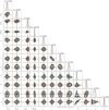 |
Fig. 14 Same as for Fig. 13, but in the case of the star-planet model. |
| In the text | |
|
Fig. 15 Best-fit star-planet model (top), RV residuals (middle), and RV curve folded at the best-fit orbital period for GJ 9689 b (bottom). |
| In the text | |
|
Fig. 16 RV semi-amplitude derived for GJ 9689 b using the star-planet model described in the text as a function of the number of observations. The shadow region indicates the 1σ uncertainties. |
| In the text | |
|
Fig. 17 Known RV planets (planetary mass versus orbital period diagram) around M dwarfs (As listed at http://exoplanet.eu/ in December 2020). Planets discovered by the HADES survey are shown as red triangles. The planet GJ 9689 b is shown as a black star. |
| In the text | |
|
Fig. 18 Histogram of derived CMF for suspected rocky planets around M dwarfs. The vertical red line shows the median of the distribution. |
| In the text | |
|
Fig. B.1 Top: GLS periodogram of the DRS RV measurements. Middle: GLS periodogram after subtracting the 18.27 d period. Bottom: GLS periodogram after subtracting the 18.27 and the 39.31 d signals. Values corresponding to a FAP of 10, 1, and 0.1% are shown with horizontal grey lines. The vertical red line indicates the period at 39.31 d, while the vertical green line shows the 18.27 d period. The first harmonic of the 39.31 d signal is shown in violet. |
| In the text | |
|
Fig. B.2 Left: autocorrelation function of RV, S-index, and Hα time series. Right: corresponding GLS diagrams. |
| In the text | |
|
Fig. B.3 Posterior distribution of the GP-only model of the S-index time series in which median and maximum a-posterior probability (MAP) have been marked (respectively, red and green line). |
| In the text | |
|
Fig. B.4 Posterior distribution of the GP-only model of the EXORAP V band photometry in which median and maximum a-posterior probability (MAP) have been marked (respectively, red and green line). |
| In the text | |
Current usage metrics show cumulative count of Article Views (full-text article views including HTML views, PDF and ePub downloads, according to the available data) and Abstracts Views on Vision4Press platform.
Data correspond to usage on the plateform after 2015. The current usage metrics is available 48-96 hours after online publication and is updated daily on week days.
Initial download of the metrics may take a while.