| Issue |
A&A
Volume 651, July 2021
|
|
|---|---|---|
| Article Number | A57 | |
| Number of page(s) | 9 | |
| Section | Galactic structure, stellar clusters and populations | |
| DOI | https://doi.org/10.1051/0004-6361/202140826 | |
| Published online | 13 July 2021 | |
G 112-43/44: A metal-poor binary star with a unique chemical composition and Helmi stream kinematics⋆
1
Stellar Astrophysics Centre, Department of Physics and Astronomy, Aarhus University, Ny Munkegade 120, 8000 Aarhus C, Denmark
e-mail: This email address is being protected from spambots. You need JavaScript enabled to view it.
2
CONACYT, Instituto de Astronomia, Universidad Nacional Autónoma de México, AP 106, Ensenada, 22800 BC, Mexico
3
Instituto de Astronomia, Universidad Nacional Autónoma de Mexico, AP 106, Ensenada 22800, BC, Mexico
Received:
18
March
2021
Accepted:
28
April
2021
Abstract
Context. Correlations between high-precision elemental abundance ratios and the kinematics of halo stars provide interesting information about the formation and early evolution of the Galaxy.
Aims. Element abundances of G 112-43/44, a metal-poor wide-orbit binary star with extreme kinematics, are revisited.
Methods. High-precision studies of the chemical compositions of 94 metal-poor dwarf stars in the solar neighbourhood are used to compare abundance ratios for G 112-43/44 with ratios for stars that have similar metallicities, taking into account the effect of deviations from local thermodynamic equilibrium on the derived abundances. Gaia EDR3 data are used to compare the kinematics.
Results. The X/Fe abundance ratios of the two components of G 112-43/44 agree within ±0.05 dex for nearly all elements, but there is a hint of a correlation between the difference in [X/H] and the elemental condensation temperature, which may be due to planet-star interactions. The Mg/Fe, Si/Fe, Ca/Fe, and Ti/Fe ratios of G 112-43/44 agree with the corresponding ratios for accreted (Gaia-Enceladus) stars, but Mn/Fe, Ni/Fe, Cu/Fe, and Zn/Fe are significantly enhanced, with Δ [Zn/Fe] reaching 0.25 dex. The kinematics show that G 112-43/44 belongs to the Helmi streams in the solar neighbourhood. In view of this, we discuss if the abundance peculiarities of G 112-43/44 can be explained by chemical enrichment from supernova events in the progenitor dwarf galaxy of the Helmi streams. Interestingly, yields calculated for a helium shell detonation Type Ia supernova model can explain the enhancement of Mn/Fe, Ni/Fe, Cu/Fe, and Zn/Fe in G 112-43/44 and three other α-poor stars in the Galactic halo with abundances from the literature, one of which has Helmi stream kinematics. However, the helium shell detonation model also predicts enhanced abundance ratios of Ca/Fe, Ti/Fe, and Cr/Fe, in disagreement with the observed ratios.
Key words: stars: abundances / stars: kinematics and dynamics / planet-star interactions / Galaxy: halo / Galaxy: formation
Based on observations made with the ESO telescopes at the La Silla Paranal Observatory under programmes 69.D0679, 70.D-0474, and 76.B-0133, and on observations made with the Nordic Optical Telescope on La Palma.
© ESO 2021
1. Introduction
High-precision studies of the chemical composition of metal-poor, high-velocity stars in the solar neighbourhood have provided interesting information about the formation and early evolution of the Milky Way. Until 25 years ago, it was believed (see the review by McWilliam 1997) that nearly all stars with [Fe/H] < −1.0 have a uniformly enhanced ratio between the abundance of α-capture elements and iron relative to the corresponding ratio for the Sun, that is [α/Fe]1 ∼ + 0.4, as expected if core collapse supernovae (SNe) are the only source of chemical enrichment at low metallicities (Kobayashi et al. 2006). Work around the beginning of the 21st century revealed, however, that there are significant variations in [α/Fe] correlated with kinematical properties; stars with high space velocities and retrograde moving stars were found to have lower [α/Fe] values than prograde moving halo stars (Nissen & Schuster 1997; Hanson et al. 1998; Fulbright 2002; Stephens & Boesgaard 2002; Gratton et al. 2003; Jonsell et al. 2005; Ishigaki et al. 2010). The differences in [α/Fe] are, however, only of the order of 0.10–0.15 dex, and with the precision obtained in the cited papers, it was unclear if there was a continuum of [α/Fe] values at a given [Fe/H] or a bimodal distribution.
This question was answered by Nissen & Schuster (2010), who, in a study of 94 high-velocity F and G dwarf stars, reached a precision of 0.02 dex for the differential values of [α/Fe] and showed that stars in the metallicity range −1.4 < [Fe/H] < −0.7 are distributed in two distinct populations, high-α and low-α halo stars. These two populations are also well separated in terms of other abundance ratios, such as [Na/Fe], [Ni/Fe], [Cu/Fe], and [Zn/Fe]. Furthermore, the low-α stars tend to move on retrograde orbits and reach larger apo-galactic distances than the high-α stars (Schuster et al. 2012). This and the decreasing trend of [α/Fe] with increasing [Fe/H], as observed in dwarf galaxies (see the review by Tolstoy et al. 2009), suggest that the low-α population has been accreted from dwarf galaxies in which Type Ia SNe start to contribute Fe at a relatively low metallicity because of a low star-formation rate. The high-α stars, on the other hand, may have formed in situ in a dissipative component with such a high star-formation rate that only Type II SNe contributed to the chemical evolution.
The findings of Nissen & Schuster (2010) have been confirmed for a larger sample of K giants with high-precision APOGEE abundances by Hawkins et al. (2015) and Hayes et al. (2018), who added [Al/Fe] as a powerful discriminator between high- and low-α stars. Furthermore, Gaia Collaboration (2018a) showed that the colour-magnitude diagram of stars with high tangential velocities, Vt > 200 km s−1, has two separated sequences in the turnoff region, the blue sequence of which corresponds to low-α stars and the redder sequence to high-α stars (Haywood et al. 2018). Another interesting result from Gaia Data Release 2 (DR2; Gaia Collaboration 2018b) was obtained by Helmi et al. (2018), who showed that the low-α stars form an elongated structure in the Toomre velocity diagram with a slightly retrograde mean rotation. Based on this, they suggested that the low-α stars are the debris of an accreted massive dwarf galaxy named ‘Gaia-Enceladus’. The high-α population was explained as having been formed in a precursor to the thick disk and heated to halo kinematics in connection with the Gaia-Enceladus merger.
In a comprehensive review, Helmi (2020) argues that the large extension in metallicity and the small width in [α/Fe] of the low-α sequence (consistent with the measurement errors of the APOGEE abundances) make it unlikely that this population consists of stars from several small-mass dwarf galaxies. Nissen & Schuster (2011) find, however, significant variations in [X/Fe] among the low-α stars. At a given [Fe/H], the variations in [X/Fe] for the high-α population correspond to the measurement errors, but for the low-α stars the variations in [Na/Fe], [Mg/Fe], [Ni/Fe], and [Cu/Fe] are two to three times larger. This can be explained if the low-α population has been accreted from at least two dwarf galaxies with different star-formation rates. Furthermore, according to Mackereth et al. (2019), APOGEE abundances provide evidence of systematic differences in [Mg/Fe], [Al/Fe], and [Ni/Fe] for low-α stars that have either high or low orbital eccentricities, and other works (Matsuno et al. 2019; Koppelman et al. 2019a; Monty et al. 2020) suggest that high-energy retrograde halo stars, belonging to the so-called Gaia-Sequoia event, stand out by having lower [Na/Fe], [Mg/Fe], and [Ca/Fe] ratios than the bulk of the Gaia-Enceladus stars. Although these variations could be related to radial abundance gradients in the Gaia-Enceladus progenitor galaxy (Koppelman et al. 2020), they can also be explained if several dwarf galaxies contributed to the low-α population. Clearly, it would be interesting to obtain additional high-precision abundances for metal-poor stars with different kinematics.
As a small contribution to this discussion, we present a detailed discussion of the metal-poor binary star G 112-43/44, which belongs to the low-α population but has enhanced abundance ratios of Mn/Fe, Ni/Fe, and Zn/Fe, according to Nissen & Schuster (2010, 2011). In Sect. 2 we use Gaia Early Data Release 3 (EDR3) data to show that G 112-43/44 belongs to one of the Helmi streams in the solar neighbourhood, and in Sect. 3 we compare the abundances of the two components with other low-α stars that have similar metallicities. In Sect. 4 we discuss how the derived [X/Fe] enhancements of G 112-43/44 can be explained, and some conclusions are presented in Sect. 5.
2. Kinematics
The components of G 112-43/44, alias BD +00 2058 A and B, are separated by 12 arcsec on the sky and have visual magnitudes of VA = 10.19 and VB = 11.17 (Schuster et al. 1993). They were listed as a common proper motion pair in Luyten (1979) and identified as a physical pair by Ryan (1992) on the basis of photometric distances and spectroscopic metallicities from Laird et al. (1988), [Fe/H] = −1.44 and −1.46, respectively. The physical connection is confirmed by Gaia satellite observations, as seen in Table 1, where data from the EDR3 (Gaia Collaboration 2016, 2021) are given. Table 1 shows that the proper motions, radial velocities, parallaxes, and the derived space velocities of the two components agree very well. Further evidence for a physical connection comes from the agreement of the chemical abundances of the two stars, as discussed in Sect. 4.
We also used Gaia EDR3 proper motions and parallaxes to re-calculate space velocities, ULSR, VLSR, and WLSR, with respect to the local standard of rest (LSR) of the other stars in Nissen & Schuster (2010). This has led to a reduction in the errors of the space velocities from typically 10–20 km s−1 to 1–2 km s−1 mainly because the Gaia distances are much more precise than the HIPPARCOS and photometric distances applied in the 2010 paper2. Furthermore, we updated the solar motion relative to the LSR to (U⊙, V⊙, W⊙) = (11.1, 12.24, 7.25) km s−1 (Schönrich et al. 2010) and the circular speed of the LSR to 232.8 km s−1 (McMillan 2017). Based on these new kinematical data, Fig. 1 shows the Vϕ–VZ diagram for stars in Nissen & Schuster (2010) that could be clearly classified as belonging to either the high-α population (blue circles) or the low-α sequence (filled red circles).
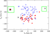 |
Fig. 1. Vϕ–VZ diagram for stars with [Fe/H] > −1.4 in Nissen & Schuster (2010). Vϕ is the Galactic rotational velocity component, Vϕ = VLSR + 232.8 km s−1, and VZ is the component perpendicular to the Galactic plane, VZ = WLSR. Stars from Nissen & Schuster (2010) belonging to the high-α sequence are shown with blue circles and those on the low-α sequence with filled red circles. G 112-43/44 is indicated with a black square. The three α-poor halo stars discussed in Sect. 4 are shown with asterisks. The green boxes indicate the location of the Helmi streams according to Koppelman et al. (2019b). |
As seen from Fig. 1, G 112-43/44 stands out from the other low-α stars by having a large (negative) velocity component perpendicular to the Galactic plane and by falling in the Vϕ − VZ box of one of the streams in the solar neighbourhood discovered by Helmi et al. (1999). The two components are included among the 40 core members of the Helmi streams with distances less than 1 kpc listed in Koppelman et al. (2019b, Table 1) by their Gaia DR2 numbers and were also associated with the Helmi streams by Jean-Baptiste et al. (2017) based on HIPPARCOS data. It is therefore likely that G 112-43/44 was formed in the progenitor galaxy of the Helmi streams. According to Koppelman et al. (2019b), this dwarf galaxy had a stellar mass of ∼108 M⊙ and was accreted 5–8 Gyr ago.
3. Element abundances
The components of G 112-43/44 were included among the 94 halo and thick-disk stars for which Nissen & Schuster (2010, 2011) derived element abundances from high signal-to-noise, S/N ∼ 200 − 300, spectra using 1D MARCS model atmospheres (Gustafsson et al. 2008) to analyse the measured equivalent widths under the assumption of local thermodynamic equilibrium (LTE). As described in detail in Nissen & Schuster (2010), the effective temperature, Teff, the surface gravity, log g, and the microturbulence, ξturb, of a given star were determined from the condition that the derived Fe abundances should have no systematic dependence on the excitation potential, the ionisation stage, or the reduced equivalent width of the Fe lines. These parameters were determined with internal precisions of σTeff ≃ 30 K, σ log g ≃ 0.05 dex, and σξturb ≃ 0.1 km s−1, and differential abundance ratios, [X/Fe], for 12 elements (Na, Mg, Si, Ca, Ti, Cr, Mn, Ni, Cu, Zn, Y, and Ba) were determined with 1σ precisions of 0.01–0.04 dex, depending on the number of lines available for a given element (see the list of lines in Table 3 of Nissen & Schuster 2011).
G 112-43/44 was found to belong to the low-α population but showed an over-abundance of Mn/Fe, Ni/Fe, and Zn/Fe relative to the other low-α stars (see Fig. 2). In the following we estimate the significance of these enhancements and discuss if G 112-43/44 deviates in other abundance ratios relative to low-α stars with similar metallicities.
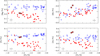 |
Fig. 2. [Mg/Fe], [Mn/Fe], [Ni/Fe], and [Zn/Fe] as a function of [Fe/H] for stars in Nissen & Schuster (2010, 2011). Stars belonging to the high-α sequence are shown with blue circles and those on the low-α sequence with filled red circles. The components of G 112-43/44 are indicated with a black square. Typical 1σ errors of the differential abundance ratios are shown at the bottom of each panel. |
Table 2 lists the atmospheric parameters and abundance ratios determined for G 112-43/44 and six low-α stars that have [Fe/H] values within ±0.10 dex of the mean [Fe/H] for G112-43/44. For most elements, the abundance ratios are LTE values from Nissen & Schuster (2010, 2011), but in the case of C and O the [X/Fe] values are from the 3D non-LTE analysis by Amarsi et al. (2019) of two high-excitation C I lines (λ5052.17 and λ5380.14 Å) and the O I triplet at λ7774 Å; in the case of Cu, abundances were adopted from Yan et al. (2016), who conducted a 1D non-LTE analysis of Cu I lines in the spectra from Nissen & Schuster (2011). There is actually one additional low-α star, G 053-41, that has a metallicity near that of G 112-43/44, but it has a very high Na/Fe ratio and low C/Fe and O/Fe ratios, suggesting that it was born as a second-generation star in a globular cluster (Ramírez et al. 2012; Nissen et al. 2014). G 053-41 was therefore excluded from the comparison with G 112-43/44.
Atmospheric parameters and abundance ratios for G 112-43/44 and the comparison stars.
In Table 2 we compare the mean [X/Fe] values for G 112-43/44 (Col. 4) with the mean [X/Fe] of the six comparison stars (Col. 11). In the case of G 112-43/44, the quoted errors of the mean [X/Fe] are calculated as ![Mathematical equation: $ \sigma \, {\text{[X/Fe]}}/ \sqrt{n} $](/articles/aa/full_html/2021/07/aa40826-21/aa40826-21-eq1.gif) , where σ [X/Fe] is the statistical 1σ error estimated from the line-to-line scatter and n = 2, except in the case of oxygen for which n = 1 because the O triplet was not covered by the spectrum of G 112-44. For the six comparison stars, the quoted errors are the standard deviation of the mean of [X/Fe]. Based on these data, the last column gives the difference between the mean [X/Fe] for G 112-43/44 and the mean [X/Fe] for the six comparison stars. The errors given are calculated as the quadratic sum of the errors of the two mean values.
, where σ [X/Fe] is the statistical 1σ error estimated from the line-to-line scatter and n = 2, except in the case of oxygen for which n = 1 because the O triplet was not covered by the spectrum of G 112-44. For the six comparison stars, the quoted errors are the standard deviation of the mean of [X/Fe]. Based on these data, the last column gives the difference between the mean [X/Fe] for G 112-43/44 and the mean [X/Fe] for the six comparison stars. The errors given are calculated as the quadratic sum of the errors of the two mean values.
The last column of Table 2 shows that the [Mn/Fe], [Ni/Fe], and [Zn/Fe] values of G 112-43/44 are enhanced relative to the corresponding mean values for the comparison stars at a confidence level of 7–8σ. [Na/Fe] and [Cu/Fe] also seem significantly enhanced (at a confidence level of 4–5σ). Furthermore, [Ba/Fe] may be lower in G 112-43/44 than in the comparison stars, but this is only significant at a level of 3σ. For the remaining elements, the mean [X/Fe] of G 112-43/44 agrees with the mean of [X/Fe] for the comparison stars within ±2σ of the estimated errors of the difference.
The largest enhancement occurs for Zn with Δ⟨[X/Fe]⟩ = 0.248. This can be seen directly from the spectra, as shown in Fig. 3, where the spectrum of G 112-43 is compared with that of one of the comparison stars, CD−51 4628. The atmospheric parameters of the two stars are similar: (Teff, log g, [Fe/H]) = (6074 K, 4.03, −1.253) for G 112-43 and (6153 K, 4.31, −1.298) for CD−51 4628. The differences in these parameters have only a minor effect on the strengths of the Fe I and Zn I lines. As can be seen, the Fe I lines are only slightly stronger in the spectrum of G 112-43, whereas the equivalent width of the Zn I line is nearly a factor of two larger.
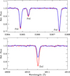 |
Fig. 3. Comparison of the spectrum of G 112-43 (red line) with that of CD−51 4628 (blue line) for three FeI lines around 5366 Å and the Zn I line at 4810.5 Å. |
As mentioned above, the abundances in Nissen & Schuster (2010, 2011) were derived by assuming LTE. Deviations from LTE (non-LTE effects) may affect the derived abundances and hence the trends of [X/Fe] as a function of [Fe/H], but the effects on differential abundances at a given [Fe/H] were expected to be small because the stars are confined to small ranges in Teff and log g. Thanks to recent detailed non-LTE studies, we now have the possibility to check this expectation in connection with the determination of abundances of G 112-43/44 relative to the comparison stars.
Table 3 lists the non-LTE corrections relative to the solar corrections, namely δ[X/H] = [X/H]non − LTE − [X/H]LTE for G 112-43 and G 112-44 in Cols. 3 and 4 and the mean correction for the comparison stars in Col. 5. The last column gives the difference in the mean correction of [X/Fe] between G 112-43/44 and the comparison stars. These corrections were obtained for the applied spectral lines by interpolation in the tables of non-LTE corrections from the listed references3.
Non-LTE corrections of abundances.
As seen from Table 3, the differences in the non-LTE corrections between G 112-43 and G 112-44 are quite small (i.e., ∼ − 0.01 to ∼ + 0.03 dex), except in the case of Cu for which the difference reaches +0.06 dex; this is caused by steeply rising non-LTE corrections for the Cu I lines as a function of increasing Teff and decreasing log g4. For oxygen there is a very significant non-LTE effect on the difference in [X/Fe] between G112-43 and the comparison stars (last column), but for the other elements the non-LTE effects on the differences in [X/Fe] between G 112-43/44 and the comparison stars lie within the statistical uncertainties given in the last column of Table 2. In particular, we note that non-LTE effects have a negligible influence on the derived over-abundance of Mn/Fe, Cu/Fe, and Zn/Fe in G 112-43/44 relative to the comparison stars. Unfortunately, there is no non-LTE study of Ni (or Y), but it would be surprising if the measured over-abundance of Ni/Fe in the G 112-43/44 pair had anything to do with non-LTE effects. The good agreement between the Ni abundance in the solar photosphere derived from an LTE analysis of Ni I lines (Scott et al. 2015) and the meteoritic abundance (Lodders 2003) suggests that non-LTE effects on Ni I lines are small. Concerning yttrium, the abundances were derived from two lines belonging to the Y II majority species, and we would therefore expect that the non-LTE effects on the derived differential Y abundances are small, such as in the case of Ba abundances derived from Ba II lines.
A notorious uncertainty in non-LTE calculations is the rate of collisions of atoms with neutral hydrogen. For some of the elements in Table 3 (C, O, Mg, Ca, and Fe), the non-LTE studies are based on new quantum-mechanical rate coefficients, but for the other elements the classical coefficients of Drawin (1969; eventually scaled by an empirical factor) were applied, which makes the non-LTE corrections somewhat uncertain. Furthermore, the corrections were calculated for 1D atmospheric models, except in the case of C and O, for which Amarsi et al. (2019) provided 3D non-LTE to 1D LTE corrections. Hence, there is room for improvements, but we do not expect 3D–1D corrections to have a significant effect on the differential abundances of G 112-43/44 relative to the comparison stars given that the stars have nearly the same [Fe/H] and have only small differences in Teff and log g.
4. Discussion
4.1. Abundance differences between G 112-43 and G 112-44
As seen from Table 2, the abundances of the two components of G 112-43/44 show good agreement. For most elements, the difference is less than, or of the order of, the 1σ error of the abundance ratios. As shown in Fig. 4, the difference in [X/H] between G 112-43 and G 112-44 seems, however, to depend on the elemental condensation temperature, Tcond (Lodders 2003). Based on a weighted least squares fit to the LTE abundances, we find a linear relation:
![Mathematical equation: $$ \begin{aligned} \Delta \mathrm{[X/H]} = -0.035 + 6.90 \, ({\pm } 3.67) 10^{-5} \cdot T_{\rm cond} \, \mathrm{dex\,K}^{-1}. \end{aligned} $$](/articles/aa/full_html/2021/07/aa40826-21/aa40826-21-eq2.gif) (1)
(1)
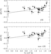 |
Fig. 4. Difference in [X/H] between G 112-43 and G 112-44 as a function of elemental condensation temperature. The upper panel refers to LTE abundances, whereas non-LTE corrections from Table 3 have been applied in the lower panel. The solid lines correspond to the fits of the data given in Eqs. (1) and (2). |
If the non-LTE corrections in Table 3 are applied, the relation becomes
![Mathematical equation: $$ \begin{aligned} \Delta \mathrm{[X/H]} = -0.008 + 5.96 \, ({\pm } 3.84) 10^{-5} \cdot T_{\rm cond} \, \mathrm{dex\,K}^{-1}. \end{aligned} $$](/articles/aa/full_html/2021/07/aa40826-21/aa40826-21-eq3.gif) (2)
(2)
In this case, Ni and Y were excluded from the fit because the non-LTE corrections are not available for these elements. As seen, the non-LTE corrections have only a small effect on the Δ[X/H] − Tcond relation. The derived slope of Δ[X/H] as a function of Tcond is, however, only significant at the 1.9σ level in the LTE case and 1.6σ in the non-LTE case.
Significant Tcond trends of the difference in [X/H] between components of co-moving twin stars have been discovered in at least seven cases (Ramírez et al. 2019), but all these stars belong to the disk population and have metallicities ranging from [Fe/H] = −0.4 to 0.4. For the halo population, there is only one co-moving pair, HD 134439/134440 with [Fe/H] ≃ −1.4, for which a Tcond trend of chemical abundances has been claimed (Chen & Zhao 2006; Chen et al. 2014), but Reggiani & Meléndez (2018) find no trend of Δ[X/H] with Tcond based on a high-precision differential abundance analysis of high-resolution spectra with S/N ∼ 250. They found, however, an average difference in [X/H] of 0.06 dex between HD 134440 and HD 134439 for 17 elements ranging from C to Ba, which they suggest could be due to the engulfment of a Jupiter-mass planet by HD 134440. In the case of G 112-43/44, the Δ[X/H] − Tcond trend in Fig. 4 could be due to the sequestration of refractory elements (Meléndez et al. 2009) in planets around G 112-44 or to the accretion of Earth-like material (Cowley et al. 2021) into the convection zone of G 112-43. Alternative explanations include dust-gas separation in star-forming clouds (Gustafsson 2018) or in proto-planetary disks (Booth & Owen 2020).
4.2. The enhancement of Mn, Ni, Cu, and Zn abundances in G 112-43/44
The [X/Fe] abundance ratios for G 112-43/44 and the comparison stars are shown in Fig. 5 on a scale where the mean [X/Fe] of the comparison stars is normalised to zero for all elements. The error bars refer to the statistical uncertainties of the differential abundance ratios as estimated in Nissen & Schuster (2010, 2011) and Amarsi et al. (2019). These errors vary from element to element depending on the number and strengths of lines available for the abundance determination. The errors are, for example, very small for nickel, for which about 25 Ni I lines are available, but are relatively large for carbon because only two weak C I lines could be applied. The errors are also large for the oxygen abundances because the O I 7774 Å triplet lines are sensitive to errors in Teff and log g.
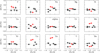 |
Fig. 5. Difference in [X/Fe] for stars in Table 2 relative to the mean of [X/Fe] for the six comparison stars as a function of [Fe/H]. G 112-43 and G 112-44 are shown with red filled circles and the comparison stars with black filled circles. The error bars refer to the 1σ uncertainties of the abundance ratios. Non-LTE corrections of [X/Fe] are included when available. |
Before making Fig. 5, we included non-LTE corrections of [X/Fe] (except for Ni and Y) for all stars, but this has only a small effect on the mean difference in [X/Fe] between G 112-43/44 and the comparison stars (see the last column of Table 3). As seen from Fig. 5, the over-abundances of [Mn/Fe], [Ni/Fe], [Cu/Fe], and [Zn/Fe] in G 112-43/44 look very significant, whereas the possible deviations of [Na/Fe] and [Ba/Fe] are less convincing because of a relatively large scatter in these abundance ratios among the comparison stars. Furthermore, we note the excellent agreement between [α/Fe] for the G 112-43/44 pair and the comparison stars.
G 112-43 (but not G 112-44) and one of our comparison stars (G 176-53) were included in a high-precision study of chemical abundances in the Milky Way thick disk and halo by Ishigaki et al. (2012, 2013). As discussed in their papers, the derived [X/Fe] values show good agreement with the corresponding values in Nissen & Schuster (2010, 2011). In particular, Ishigaki et al. found the same high Zn/Fe ratio of ∼0.3 dex for G 112-43 as in the present paper, and they also found [Mn/Fe] and [Ni/Fe] to be enhanced in G 112-43 relative to G 176-53 (the abundance of Cu in G 176-53 was not determined by Ishigaki et al.).
Interestingly, three other α-poor stars in the Galactic halo have the same pattern of Mn, Ni, and Zn enhancements relative to Fe as G 112-43/44. Ivans et al. (2003) found G 4-36 (a turnoff star with Teff = 5975 K and [Fe/H] = −1.94) and BPS CS 22966-43 (a blue metal-poor star with Teff = 7400 K and [Fe/H] = −1.91) to be enhanced in Mn/Fe, Ni/Fe, and Zn/Fe relative to Milky Way stars with similar metallicities (see their Figs. 10 and 11). Honda et al. (2011) found BPS BS 16920-17 (a giant star with Teff = 4760 K and [Fe/H] = −3.1) to have similar enhancements relative to a well-known halo giant, HD 4306, that has Teff = 4810 K and [Fe/H] = −2.8. For all three stars, the enhancement in Zn is Δ[Zn/Fe] ∼ 0.9, and Δ[Mn/Fe] and Δ[Ni/Fe] are at a level of 0.5 dex. The abundance of Cu was not determined for the three stars.
High Zn/Fe ratios, [Zn/Fe] ∼ 0.5, in very metal-poor stars (Cayrel et al. 2004; Nissen et al. 2007) have been explained as being due to hypernovae (Umeda & Nomoto 2002), that is, massive core-collapse SNe with explosion energies E ∼ 1052 erg, which is ten times higher than those of normal Type II SNe. However, a hypernova cannot explain the enhancement of Mn/Fe, Ni/Fe, or Cu/Fe; as seen from Fig. 8 in the review of nucleosynthesis by Nomoto et al. (2013), the yields of [Mn/Fe] and [Cu/Fe] are around −0.7 dex and that of [Ni/Fe] is ∼ − 0.2 dex. Figure 8 in Nomoto et al. (2013) also shows that pair-instability SNe, faint SNe, and the classical W7 single-degenerate Chandrasekhar-mass (MCh) Type Ia SN model of Iwamoto et al. (1999) all fail to explain the distribution of Δ[X/Fe] for Mn, Ni, Cu, and Zn in G 112-43/44 and the three α-poor stars discussed above. There are, however, other models of Type Ia SNe with different nucleosynthesis yields, as recently analysed by Lach et al. (2020). Among the various possible scenarios – including single and double degenerate models with both MCh and sub-MCh masses and different explosion mechanisms, for which [X/Fe] is shown in their Fig. 3 – one model produces enhanced [X/Fe] values for Mn, Ni, Cu, and Zn. This so-called HeD-S model consists of a sub-MCh mass white dwarf with a prominent helium shell in which a detonation takes place without triggering an explosion in the CO core.
The calculated [X/Fe] yields of iron-peak elements5 for the HeD-S model are shown in Fig. 6 in comparison with the observed Δ[X/Fe] values for G 112-43/44 and the three α-poor halo stars. As seen, there is satisfactory agreement between the HeD-S model predictions and the observed enhancements of [Ni/Fe] and [Zn/Fe] for the three α-poor stars, and the observed enhancement of Mn/Fe is a bit higher. The [X/Fe] enhancements for G 112-43/44 (including [Cu/Fe]) are not as large as the [X/Fe] yield predictions for the HeD-S model but have a similar relative distribution. Such an offset may occur if the elements produced by the HeD-S SN are mixed with a relatively large amount of gas produced by the kind of ‘normal’ Type Ia SNe that control the chemical evolution of iron-peak elements for the stellar system in which G 112-43/44 was born.
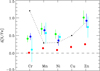 |
Fig. 6. Enhancements of iron-peak elements for G 112-43/44 and three α-poor halo stars in comparison with the [X/Fe] yield distribution (dotted line) calculated by Lach et al. (2020) for a pure helium shell detonation Type Ia SN model. Red symbols refer to data for G 112-43/44, blue symbols to G 4-36, green symbols to BPS CS 22966-43, and cyan symbols to BPS BS 16920-17. The error bars refer to statistical uncertainties in the abundance determinations. |
The HeD-S model cannot, however, explain all abundances in G 112-43/44 and the three α-poor halo stars. As seen from Fig. 6, the predicted yield of [Cr/Fe] is much higher than the observed Δ[Cr/Fe] enhancements, and the HeD-S model also predicts super-solar values of [Ca/Fe] and [Ti/Fe], 0.5 and 1.8 dex respectively, in strong disagreement with the much lower observational values. It remains to be seen if this problem can be solved with a revised model for a He shell detonation Type Ia SN. In any case, we think it is likely that the Mn/Fe, Ni/Fe, Cu/Fe, and Zn/Fe enhancements in G 112-43/44 and the three α-poor stars are caused by element contribution from a special kind of SN to pockets of gas from which these stars were formed. Such inhomogeneous mixing of SN products is more likely to affect the chemical evolution of dwarf galaxies than higher-mass systems because in lower-mass galaxies the gas has a relatively long cooling time, resulting in episodic star-formation bursts (Revaz et al. 2009; Venn et al. 2012). In view of this, it is interesting that G 112-43/44, as a member of the Helmi streams, was probably born in a dwarf galaxy and that one of the three α-poor halo stars with enhancements of Mn/Fe, Ni/Fe, and Zn/Fe also has Helmi stream kinematics6, as seen from Fig. 1. G 4-36 and BPS BS 16920-17 have kinematics similar to stars belonging to the Gaia-Enceladus population, but BPS CS 22966-43 lies in the Helmi box with positive VZ.
Not all stars belonging to the Helmi streams have unusual abundances. Roederer et al. (2010) made a detailed abundance analysis of 12 subgiant and giant stars with Helmi stream kinematics, and Gull et al. (2021) recently added seven stars to this work. Within the typical errors of the abundance determinations (0.10–0.15 dex), [Mn/Fe], [Ni/Fe], [Cu/Fe], and [Zn/Fe] agree with the [X/Fe]-[Fe/H] trends of Galactic halo stars. The stars investigated, however, have [Fe/H] ≲ −1.5 and high [α/Fe] ratios (e.g., [Mg/Fe] ∼ 0.3), so it remains to be seen if the Helmi streams contain a population of low-α stars at higher metallicities and if some of these stars have over-abundances of Mn, Ni, Cu, and Zn relative to Fe.
Low-α stars are well known in dwarf galaxies (see the review by Tolstoy et al. 2009). In the Sculptor dSph galaxy, for example, [Mg/Fe] shows a declining metallicity trend from [Mg/Fe] ≃ 0.4 at [Fe/H] = −1.8 to [Mg/Fe] ≃ −0.2 at [Fe/H] = −1.0. Interestingly, Skúladóttir et al. (2017) find indications of a cosmic scatter in [Zn/Fe] of the Sculptor stars (i.e., from about −0.6 dex to +0.4 dex) and a positive correlation between [Ni/Fe] and [Zn/Fe]. At a distance of ∼85 kpc, the giants observed in Sculptor are, however, faint (17.0 < V < 18.5), and the errors of [Zn/Fe] are of the order of ±0.3 dex. It will require more precise [Ni/Fe] and [Zn/Fe] values as well as an improved precision of [Mn/Fe] values (North et al. 2012) to verify if stars with enhanced Mn/Fe, Ni/Fe, and Zn/Fe ratios are present in Sculptor.
Another interesting case is the ultra-faint dwarf galaxy Horologium I, in which Nagasawa et al. (2018) found three very metal-poor ([Fe/H] ∼ −2.5) giant stars that are α-poor ([Mg/Fe] and [Ca/Fe] ≃ 0.0) and enhanced in [Mn/Fe] by about 0.4 dex relative to Galactic halo stars. However, their [Ni/Fe] ratios seem to be normal, and their Cu and Zn abundances were not determined. Again, we need more precise abundances, including those of Cu and Zn, to make conclusions about the possible existence of stars in Horologium I with peculiar abundance ratios among the iron-peak elements.
5. Summary and conclusions
In this paper we have made a high-precision study of elemental abundance ratios for the components of the low-α metal-poor binary star G 112-43/44 in comparison with abundance ratios for six low-α halo stars that have nearly the same metallicity and similar Teff and log g values. Non-LTE effects on the derived differential abundance ratios were considered, but they were found to be small, except for [O/Fe] (see Table 3). As a main result, we find that the abundance ratios of Mn, Ni, Cu, and Zn with respect to Fe are significantly enhanced in G 112-43/44 relative to the comparison stars: Δ[Mn/Fe] = 0.14 ± 0.02, Δ[Ni/Fe] = 0.09 ± 0.01, Δ[Cu/Fe] = 0.18 ± 0.04, and Δ[Zn/Fe] = 0.25 ± 0.03.
From a literature search, we found three other α-poor halo stars, G 4-36, BPS CS 22966-43 (Ivans et al. 2003), and BPS BS 16920-17 (Honda et al. 2011), with enhanced abundances of Mn, Ni, and Zn relative to Fe. The errors of the abundance ratios are much higher than in our study of G 112-43/44 (0.10–0.20 dex), but the amplitude of the enhancements is also higher, reaching Δ[Zn/Fe] ∼ 1.0. As such, the significance of the abundance peculiarities is still high.
Interestingly, two of the four stars with enhanced [X/Fe] values for the iron-peak elements (G 112-43/44 and BPS CS 22966-43) have very high velocity components in a direction perpendicular to the Galactic plane, indicating that they are members of the Helmi streams. This suggests that such stars occur at a higher frequency in the progenitor dwarf galaxy of the Helmi streams than in the more massive Gaia-Enceladus galaxy, which is responsible for most of the low-α halo stars in the solar neighbourhood. In view of this, it would be interesting to carry out a high-precision abundance study of K giants in dwarf galaxies with a large population of low-alpha stars, such as Fornax and Sculptor. Due to the large distances of these systems, this would, however, require extremely large telescopes to obtain high-resolution spectra with sufficiently high S/N to detect over-abundances of Mn, Ni, Cu, and Zn with respect to Fe. It would also be interesting to extend the abundance study of members of the Helmi streams by Roederer et al. (2010) to stars with [Fe/H] > −1.5, at which metallicity one would expect that Type Ia SNe start contributing to the abundance of the iron-peak elements in the progenitor galaxy of the streams. We note that the metallicity distribution of members of the Helmi streams peaks at [Fe/H] ≃ −1.5 with a tail up to [Fe/H] ∼ −0.5 (Koppelman et al. 2019b).
It is unclear which SN type can produce an over-abundance of Mn, Ni, Cu, and Zn relative to Fe. Hypernovae have been proposed (Umeda & Nomoto 2002) as the source of enhanced Zn/Fe values in very metal-poor stars, but they cannot explain the enhancement of Mn/Fe, Ni/Fe, or Cu/Fe (Nomoto et al. 2013). The pure helium shell detonation Type Ia SN model of Lach et al. (2020) is a more promising candidate (see Fig. 6), but this model also predicts super-solar ratios of Ca/Fe, Ti/Fe, and Cr/Fe, which are not found for the four stars discussed in this paper. It would be interesting to investigate if the helium shell detonation model can be modified to produce solar ratios of Ca/Fe, Ti/Fe, and Cr/Fe while still producing enhanced ratios of Mn/Fe, Ni/Fe, Cu/Fe, and Zn/Fe.
As an additional result, we have found that the components of the G 112-43/44 binary star do not have exactly the same abundance of elements and that the difference seems to be correlated with the elemental condensation temperature (see Fig. 4). The Δ[X/H] − Tcond slope is, however, only significant at a confidence level of 1.6σ when differential non-LTE corrections are applied. One would need to increase the S/N of the spectra from the ∼300 in this paper to ∼600 to determine if the Tcond slope is significant. It would also be important to observe the O I triplet at 7774 Å for both stars in order to determine the difference in the O abundance because oxygen has a low condensation temperature (Tcond = 180 K), similar to that of carbon (Tcond = 40 K). If the Δ[X/H] − Tcond trend were confirmed, it would show that abundance differences correlated with Tcond also occur between components of wide-orbit binaries belonging to the metal-poor halo population; this has already been found for several binaries that belong to the thin disk population (Ramírez et al. 2019). Given that these trends may be due to star-planet interactions, the detection of a Δ[X/H] − Tcond trend for a halo binary star would be interesting.
In this paper ‘α’ denotes the mean abundance of Mg, Si, Ca, and Ti.
Exceptions are HD 106516, HD 163810, and HD 219617, for which Gaia parallaxes are not available.
For the Bergemann et al. references, Spectrum Tools at http://nlte.mpia.de was used for the interpolation.
G 112-43 is a more evolved star, with δTeff = 255 K and δ log g = − 0.22 dex relative to G 112-44.
Cobalt is not included because its abundance has not been determined for G 112-43/44 or BPS CS 22966-43 and is very uncertain for G 4-36 and BPS BS 16920-17.
Space velocities were calculated based on Gaia EDR3 data supplemented with radial velocities, RV = −277 ± 10 km s−1 for BPS CS 22966-43 (Wilhelm et al. 1999) and RV = −210 ± 10 km s−1 for BPS BS 16920-17 (Allende Prieto et al. 2000).
Acknowledgments
The referee is thanked for a constructive and helpful report. Funding for the Stellar Astrophysics Centre is provided by The Danish National Research Foundation (Grant agreement no.: DNRF106). This research has made use of the SIMBAD database, operated at CDS, Strasbourg, France, as well as data from the European Space Agency (ESA) mission Gaia (https://www.cosmos.esa.int/gaia), processed by the Gaia Data Processing and Analysis Consortium (DPAC, https://www.cosmos.esa.int/web/gaia/dpac/consortium). Funding for the DPAC has been provided by national institutions, in particular the institutions participating in the Gaia Multilateral Agreement.
References
- Allende Prieto, C., Rebolo, R., García López, R. J., et al. 2000, AJ, 120, 1516 [NASA ADS] [CrossRef] [Google Scholar]
- Amarsi, A. M., Lind, K., Asplund, M., Barklem, P. S., & Collet, R. 2016, MNRAS, 463, 1518 [Google Scholar]
- Amarsi, A. M., Nissen, P. E., & Skúladóttir, Á. 2019, A&A, 630, A104 [NASA ADS] [CrossRef] [EDP Sciences] [Google Scholar]
- Bergemann, M. 2011, MNRAS, 413, 2184 [NASA ADS] [CrossRef] [Google Scholar]
- Bergemann, M., & Cescutti, G. 2010, A&A, 522, A9 [NASA ADS] [CrossRef] [EDP Sciences] [Google Scholar]
- Bergemann, M., & Gehren, T. 2008, A&A, 492, 823 [NASA ADS] [CrossRef] [EDP Sciences] [Google Scholar]
- Bergemann, M., Kudritzki, R.-P., Würl, M., et al. 2013, ApJ, 764, 115 [Google Scholar]
- Bergemann, M., Collet, R., Amarsi, A. M., et al. 2017, ApJ, 847, 15 [NASA ADS] [CrossRef] [Google Scholar]
- Booth, R. A., & Owen, J. E. 2020, MNRAS, 493, 5079 [CrossRef] [Google Scholar]
- Cayrel, R., Depagne, E., Spite, M., et al. 2004, A&A, 416, 1117 [NASA ADS] [CrossRef] [EDP Sciences] [Google Scholar]
- Chen, Y. Q., & Zhao, G. 2006, MNRAS, 370, 2091 [CrossRef] [Google Scholar]
- Chen, Y., King, J. R., & Boesgaard, A. M. 2014, PASP, 126, 1010 [CrossRef] [Google Scholar]
- Cowley, C. R., Bord, D. J., & Yüce, K. 2021, AJ, 161, 142 [CrossRef] [Google Scholar]
- Drawin, H. W. 1969, Z. Phys., 225, 483 [NASA ADS] [CrossRef] [EDP Sciences] [Google Scholar]
- Fulbright, J. P. 2002, AJ, 123, 404 [NASA ADS] [CrossRef] [Google Scholar]
- Gaia Collaboration (Prusti, T., et al.) 2016, A&A, 595, A1 [NASA ADS] [CrossRef] [EDP Sciences] [Google Scholar]
- Gaia Collaboration (Babusiaux, C., et al.) 2018a, A&A, 616, A10 [NASA ADS] [CrossRef] [EDP Sciences] [Google Scholar]
- Gaia Collaboration (Brown, A. G. A., et al.) 2018b, A&A, 616, A1 [NASA ADS] [CrossRef] [EDP Sciences] [Google Scholar]
- Gaia Collaboration (Brown, A. G. A., et al.) 2021, A&A, 649, A1 [NASA ADS] [CrossRef] [EDP Sciences] [Google Scholar]
- Gratton, R. G., Carretta, E., Desidera, S., et al. 2003, A&A, 406, 131 [NASA ADS] [CrossRef] [EDP Sciences] [Google Scholar]
- Gull, M., Frebel, A., Hinojosa, K., et al. 2021, ApJ, 912, 52 [CrossRef] [Google Scholar]
- Gustafsson, B. 2018, A&A, 620, A53 [CrossRef] [EDP Sciences] [Google Scholar]
- Gustafsson, B., Edvardsson, B., Eriksson, K., et al. 2008, A&A, 486, 951 [NASA ADS] [CrossRef] [EDP Sciences] [Google Scholar]
- Hanson, R. B., Sneden, C., Kraft, R. P., & Fulbright, J. 1998, AJ, 116, 1286 [NASA ADS] [CrossRef] [Google Scholar]
- Hawkins, K., Jofré, P., Masseron, T., & Gilmore, G. 2015, MNRAS, 453, 758 [NASA ADS] [CrossRef] [Google Scholar]
- Hayes, C. R., Majewski, S. R., Shetrone, M., et al. 2018, ApJ, 852, 49 [NASA ADS] [CrossRef] [Google Scholar]
- Haywood, M., Di Matteo, P., Lehnert, M., et al. 2018, A&A, 618, A78 [NASA ADS] [CrossRef] [EDP Sciences] [Google Scholar]
- Helmi, A. 2020, ARA&A, 58, 205 [Google Scholar]
- Helmi, A., White, S. D. M., de Zeeuw, P. T., & Zhao, H. 1999, Nature, 402, 53 [NASA ADS] [CrossRef] [Google Scholar]
- Helmi, A., Babusiaux, C., Koppelman, H. H., et al. 2018, Nature, 563, 85 [NASA ADS] [CrossRef] [Google Scholar]
- Honda, S., Aoki, W., Beers, T. C., & Takada-Hidai, M. 2011, ApJ, 730, 77 [NASA ADS] [CrossRef] [Google Scholar]
- Ishigaki, M., Chiba, M., & Aoki, W. 2010, PASJ, 62, 143 [NASA ADS] [Google Scholar]
- Ishigaki, M. N., Chiba, M., & Aoki, W. 2012, ApJ, 753, 64 [NASA ADS] [CrossRef] [Google Scholar]
- Ishigaki, M. N., Aoki, W., & Chiba, M. 2013, ApJ, 771, 67 [NASA ADS] [CrossRef] [Google Scholar]
- Ivans, I. I., Sneden, C., James, C. R., et al. 2003, ApJ, 592, 906 [NASA ADS] [CrossRef] [Google Scholar]
- Iwamoto, K., Brachwitz, F., Nomoto, K., et al. 1999, ApJS, 125, 439 [NASA ADS] [CrossRef] [MathSciNet] [Google Scholar]
- Jean-Baptiste, I., Di Matteo, P., Haywood, M., et al. 2017, A&A, 604, A106 [NASA ADS] [CrossRef] [EDP Sciences] [Google Scholar]
- Jonsell, K., Edvardsson, B., Gustafsson, B., et al. 2005, A&A, 440, 321 [NASA ADS] [CrossRef] [EDP Sciences] [Google Scholar]
- Kobayashi, C., Umeda, H., Nomoto, K., Tominaga, N., & Ohkubo, T. 2006, ApJ, 653, 1145 [NASA ADS] [CrossRef] [Google Scholar]
- Koppelman, H. H., Helmi, A., Massari, D., Price-Whelan, A. M., & Starkenburg, T. K. 2019a, A&A, 631, L9 [NASA ADS] [CrossRef] [EDP Sciences] [Google Scholar]
- Koppelman, H. H., Helmi, A., Massari, D., Roelenga, S., & Bastian, U. 2019b, A&A, 625, A5 [NASA ADS] [CrossRef] [EDP Sciences] [Google Scholar]
- Koppelman, H. H., Bos, R. O. Y., & Helmi, A. 2020, A&A, 642, L18 [CrossRef] [EDP Sciences] [Google Scholar]
- Korotin, S. A., Andrievsky, S. M., Hansen, C. J., et al. 2015, A&A, 581, A70 [NASA ADS] [CrossRef] [EDP Sciences] [Google Scholar]
- Lach, F., Röpke, F. K., Seitenzahl, I. R., et al. 2020, A&A, 644, A118 [CrossRef] [EDP Sciences] [Google Scholar]
- Laird, J. B., Carney, B. W., & Latham, D. W. 1988, AJ, 95, 1843 [NASA ADS] [CrossRef] [Google Scholar]
- Lind, K., Asplund, M., Barklem, P. S., & Belyaev, A. K. 2011, A&A, 528, A103 [NASA ADS] [CrossRef] [EDP Sciences] [Google Scholar]
- Lindegren, L., Bastian, U., Biermann, M., et al. 2021, A&A, 649, A4 [EDP Sciences] [Google Scholar]
- Lodders, K. 2003, ApJ, 591, 1220 [Google Scholar]
- Luyten, W. J. 1979, NLTT catalogue. Volume_I. +90_to_+30_. Volume._II. +30_to_0_ (Minneapolis: Univ. Minnesota) [Google Scholar]
- Mackereth, J. T., Schiavon, R. P., Pfeffer, J., et al. 2019, MNRAS, 482, 3426 [NASA ADS] [CrossRef] [Google Scholar]
- Mashonkina, L., Sitnova, T., & Belyaev, A. K. 2017, A&A, 605, A53 [NASA ADS] [CrossRef] [EDP Sciences] [Google Scholar]
- Matsuno, T., Aoki, W., & Suda, T. 2019, ApJ, 874, L35 [NASA ADS] [CrossRef] [Google Scholar]
- McMillan, P. J. 2017, MNRAS, 465, 76 [NASA ADS] [CrossRef] [Google Scholar]
- McWilliam, A. 1997, ARA&A, 35, 503 [NASA ADS] [CrossRef] [Google Scholar]
- Meléndez, J., Asplund, M., Gustafsson, B., & Yong, D. 2009, ApJ, 704, L66 [NASA ADS] [CrossRef] [Google Scholar]
- Monty, S., Venn, K. A., Lane, J. M. M., Lokhorst, D., & Yong, D. 2020, MNRAS, 497, 1236 [CrossRef] [Google Scholar]
- Nagasawa, D. Q., Marshall, J. L., Li, T. S., et al. 2018, ApJ, 852, 99 [NASA ADS] [CrossRef] [Google Scholar]
- Nissen, P. E., & Schuster, W. J. 1997, A&A, 326, 751 [NASA ADS] [Google Scholar]
- Nissen, P. E., & Schuster, W. J. 2010, A&A, 511, L10 [NASA ADS] [CrossRef] [EDP Sciences] [Google Scholar]
- Nissen, P. E., & Schuster, W. J. 2011, A&A, 530, A15 [NASA ADS] [CrossRef] [EDP Sciences] [Google Scholar]
- Nissen, P. E., Akerman, C., Asplund, M., et al. 2007, A&A, 469, 319 [NASA ADS] [CrossRef] [EDP Sciences] [Google Scholar]
- Nissen, P. E., Chen, Y. Q., Carigi, L., Schuster, W. J., & Zhao, G. 2014, A&A, 568, A25 [NASA ADS] [CrossRef] [EDP Sciences] [Google Scholar]
- Nomoto, K., Kobayashi, C., & Tominaga, N. 2013, ARA&A, 51, 457 [Google Scholar]
- North, P., Cescutti, G., Jablonka, P., et al. 2012, A&A, 541, A45 [NASA ADS] [CrossRef] [EDP Sciences] [Google Scholar]
- Ramírez, I., Meléndez, J., & Chanamé, J. 2012, ApJ, 757, 164 [Google Scholar]
- Ramírez, I., Khanal, S., Lichon, S. J., et al. 2019, MNRAS, 490, 2448 [CrossRef] [Google Scholar]
- Reggiani, H., & Meléndez, J. 2018, MNRAS, 475, 3502 [Google Scholar]
- Revaz, Y., Jablonka, P., Sawala, T., et al. 2009, A&A, 501, 189 [NASA ADS] [CrossRef] [EDP Sciences] [Google Scholar]
- Roederer, I. U., Sneden, C., Thompson, I. B., Preston, G. W., & Shectman, S. A. 2010, ApJ, 711, 573 [NASA ADS] [CrossRef] [Google Scholar]
- Ryan, S. G. 1992, AJ, 104, 1144 [NASA ADS] [CrossRef] [Google Scholar]
- Schönrich, R., Binney, J., & Dehnen, W. 2010, MNRAS, 403, 1829 [NASA ADS] [CrossRef] [Google Scholar]
- Schuster, W. J., Parrao, L., & Contreras Martinez, M. E. 1993, A&AS, 97, 951 [NASA ADS] [Google Scholar]
- Schuster, W. J., Moreno, E., Nissen, P. E., & Pichardo, B. 2012, A&A, 538, A21 [NASA ADS] [CrossRef] [EDP Sciences] [Google Scholar]
- Scott, P., Asplund, M., Grevesse, N., Bergemann, M., & Sauval, A. J. 2015, A&A, 573, A26 [NASA ADS] [CrossRef] [EDP Sciences] [Google Scholar]
- Skúladóttir, Á., Tolstoy, E., Salvadori, S., Hill, V., & Pettini, M. 2017, A&A, 606, A71 [NASA ADS] [CrossRef] [EDP Sciences] [Google Scholar]
- Stephens, A., & Boesgaard, A. M. 2002, AJ, 123, 1647 [NASA ADS] [CrossRef] [Google Scholar]
- Takeda, Y., Hashimoto, O., Taguchi, H., et al. 2005, PASJ, 57, 751 [NASA ADS] [Google Scholar]
- Tolstoy, E., Hill, V., & Tosi, M. 2009, ARA&A, 47, 371 [NASA ADS] [CrossRef] [Google Scholar]
- Umeda, H., & Nomoto, K. 2002, ApJ, 565, 385 [NASA ADS] [CrossRef] [Google Scholar]
- Venn, K. A., Shetrone, M. D., Irwin, M. J., et al. 2012, ApJ, 751, 102 [NASA ADS] [CrossRef] [Google Scholar]
- Wilhelm, R., Beers, T. C., Sommer-Larsen, J., et al. 1999, AJ, 117, 2329 [NASA ADS] [CrossRef] [Google Scholar]
- Yan, H. L., Shi, J. R., Nissen, P. E., & Zhao, G. 2016, A&A, 585, A102 [NASA ADS] [CrossRef] [EDP Sciences] [Google Scholar]
All Tables
Atmospheric parameters and abundance ratios for G 112-43/44 and the comparison stars.
All Figures
|
Fig. 1. Vϕ–VZ diagram for stars with [Fe/H] > −1.4 in Nissen & Schuster (2010). Vϕ is the Galactic rotational velocity component, Vϕ = VLSR + 232.8 km s−1, and VZ is the component perpendicular to the Galactic plane, VZ = WLSR. Stars from Nissen & Schuster (2010) belonging to the high-α sequence are shown with blue circles and those on the low-α sequence with filled red circles. G 112-43/44 is indicated with a black square. The three α-poor halo stars discussed in Sect. 4 are shown with asterisks. The green boxes indicate the location of the Helmi streams according to Koppelman et al. (2019b). |
| In the text | |
|
Fig. 2. [Mg/Fe], [Mn/Fe], [Ni/Fe], and [Zn/Fe] as a function of [Fe/H] for stars in Nissen & Schuster (2010, 2011). Stars belonging to the high-α sequence are shown with blue circles and those on the low-α sequence with filled red circles. The components of G 112-43/44 are indicated with a black square. Typical 1σ errors of the differential abundance ratios are shown at the bottom of each panel. |
| In the text | |
|
Fig. 3. Comparison of the spectrum of G 112-43 (red line) with that of CD−51 4628 (blue line) for three FeI lines around 5366 Å and the Zn I line at 4810.5 Å. |
| In the text | |
|
Fig. 4. Difference in [X/H] between G 112-43 and G 112-44 as a function of elemental condensation temperature. The upper panel refers to LTE abundances, whereas non-LTE corrections from Table 3 have been applied in the lower panel. The solid lines correspond to the fits of the data given in Eqs. (1) and (2). |
| In the text | |
|
Fig. 5. Difference in [X/Fe] for stars in Table 2 relative to the mean of [X/Fe] for the six comparison stars as a function of [Fe/H]. G 112-43 and G 112-44 are shown with red filled circles and the comparison stars with black filled circles. The error bars refer to the 1σ uncertainties of the abundance ratios. Non-LTE corrections of [X/Fe] are included when available. |
| In the text | |
|
Fig. 6. Enhancements of iron-peak elements for G 112-43/44 and three α-poor halo stars in comparison with the [X/Fe] yield distribution (dotted line) calculated by Lach et al. (2020) for a pure helium shell detonation Type Ia SN model. Red symbols refer to data for G 112-43/44, blue symbols to G 4-36, green symbols to BPS CS 22966-43, and cyan symbols to BPS BS 16920-17. The error bars refer to statistical uncertainties in the abundance determinations. |
| In the text | |
Current usage metrics show cumulative count of Article Views (full-text article views including HTML views, PDF and ePub downloads, according to the available data) and Abstracts Views on Vision4Press platform.
Data correspond to usage on the plateform after 2015. The current usage metrics is available 48-96 hours after online publication and is updated daily on week days.
Initial download of the metrics may take a while.