| Issue |
A&A
Volume 651, July 2021
|
|
|---|---|---|
| Article Number | A12 | |
| Number of page(s) | 18 | |
| Section | Astrophysical processes | |
| DOI | https://doi.org/10.1051/0004-6361/202040228 | |
| Published online | 01 July 2021 | |
X-ray emission from magnetized neutron star atmospheres at low mass-accretion rates
I. Phase-averaged spectrum
1
Dr. Karl Remeis-Observatory & ECAP, University of Erlangen-Nuremberg, Sternwartstr. 7, 96049 Bamberg, Germany
e-mail: ekaterina.sokolova-lapa@fau.de
2
Sternberg Astronomical Institute, M. V. Lomonosov Moscow State University, Universitetskij pr., 13, Moscow 119992, Russia
3
Kazan Federal University, 420008 Kazan, Russia
4
European Space Astronomy Center (ESA/ESAC), Science Operations Department, Villanueva de la Cañada, 28691 Madrid, Spain
5
Cahill Center for Astronomy and Astrophysics, California Institute of Technology, Pasadena, CA 91125, USA
6
CRESST, Department of Physics, and Center for Space Science and Technology, UMBC, Baltimore, MD 21250, USA
7
NASA Goddard Space Flight Center, Astrophysics Science Division, Greenbelt, MD 20771, USA
8
Department of Physics & Astronomy, George Mason University, Fairfax, VA 22030-4444, USA
9
Space Science Division, Naval Research Laboratory, Washington, DC 20375-5352, USA
10
NASA Marshall Space Flight Center, NSSTC, 320 Sparkman Drive, Huntsville, AL 35805, USA
11
Universities Space Research Association, Science and Technology Institute, 320 Sparkman Drive, Huntsville, AL 35805, USA
Received:
23
December
2020
Accepted:
13
April
2021
Recent observations of X-ray pulsars at low luminosities allow, for the first time, the comparison of theoretical models of the emission from highly magnetized neutron star atmospheres at low mass-accretion rates (Ṁ ≲ 1015 g s−1) with the broadband X-ray data. The purpose of this paper is to investigate spectral formation in the neutron star atmosphere at low Ṁ and to conduct a parameter study of the physical properties of the emitting region. We obtain the structure of the static atmosphere, assuming that Coulomb collisions are the dominant deceleration process. The upper part of the atmosphere is strongly heated by the braking plasma, reaching temperatures of 30–40 keV, while its denser isothermal interior is much cooler (∼2 keV). We numerically solve the polarized radiative transfer in the atmosphere with magnetic Compton scattering, free–free processes, and nonthermal cyclotron emission due to possible collisional excitations of electrons. The strongly polarized emitted spectrum has a double-hump shape that is observed in low-luminosity X-ray pulsars. A low-energy “thermal” component is dominated by extraordinary photons that can leave the atmosphere from deeper layers because of their long mean free path at soft energies. We find that a high-energy component is formed because of resonant Comptonization in the heated nonisothermal part of the atmosphere even in the absence of collisional excitations. However, these latter, if present, affect the ratio of the two components. A strong cyclotron line originates from the optically thin, uppermost zone. A fit of the model to NuSTAR and Swift/XRT observations of GX 304−1 provides an accurate description of the data with reasonable parameters. The model can thus reproduce the characteristic double-hump spectrum observed in low-luminosity X-ray pulsars and provides insights into spectral formation.
Key words: X-rays: binaries / stars: neutron / methods: numerical / radiative transfer / magnetic fields / polarization
© ESO 2021
1. Introduction
Accretion-powered X-ray pulsars have been known for decades as binary systems which consist of a rotating highly magnetized neutron star and a donor star companion (e.g., Zel’dovich & Shakura 1969; Basko & Sunyaev 1975). The strong magnetic fields of the neutron stars in high-mass X-ray binaries (HMXBs) significantly affect the accretion of matter from the donor, which is typically an early-type (O/B) star. Close to the compact object, in the magnetosphere of the neutron star, the dynamics of the accretion flow are dominated by the magnetic field of the neutron star. The accreting material couples to the magnetic field lines and is channeled down onto the magnetic poles of the neutron star. The matter is decelerated from its free-fall velocity of ∼0.7c in an accretion column or at the surface of the neutron star. The properties of the column depend on the mass-accretion rate (e.g., Burnard et al. 1991; Becker et al. 2012; Postnov et al. 2015a; Mushtukov et al. 2015). It is well understood that at high accretion rates of Ṁ ≳ 1017 g s−1 radiation pressure plays a major role in decelerating the matter (Davidson 1973; Basko & Sunyaev 1976; Wang & Frank 1981) in the accretion column. The accretion flow loses its energy gradually by passing through the extensive radiative shock. See Becker & Wolff (2007), Wolff et al. (2016), Farinelli et al. (2016), and Gornostaev (2021) for accretion column models in this high mass-accretion rate regime. At lower accretion rates, Ṁ ∼ 1015 − 1017 g s−1, it is possible that matter is decelerated by passing through a collisionless shock (Langer & Rappaport 1982; Bykov & Krasil’Shchikov 2004; Vybornov et al. 2017). In this case, the gas shock is discontinuous with post-shock velocity ∼vff. The aftershock flow is decelerated to rest by Coulomb collisions. Soft thermal X-ray photons emitted from the thermalized region near the surface of the neutron star, as well as photons produced by free–free and cyclotron emission, are then reprocessed in the column by Compton scattering to produce the harder X-rays emerging from the column. At even lower mass-accretion rates, the accretion flow approaches the neutron star surface at free-fall velocity and then rapidly decelerates in the nearly static atmosphere by Coulomb collisions (Zel’dovich & Shakura 1969, hereafter ZS69).
The extreme magnetic field of the neutron star significantly affects both the hydrodynamical characteristics of the accretion flow and the photon–electron interactions inside the plasma. In the presence of strong magnetic fields, photon scattering, absorption, and emission become resonant processes because of the quantization of the electron motion perpendicular to the magnetic field on Landau levels. As a result, the cross sections for magnetic Compton scattering and magnetic free–free absorption are strongly energy and polarization dependent and highly anisotropic (Herold 1979; Nagel 1980; Daugherty & Harding 1986; Bussard et al. 1986; Schwarm et al. 2017). The resonant nature of the scattering process is also responsible for the formation of cyclotron resonance scattering features (CRSFs), commonly referred to as cyclotron lines, which are observed in the spectra of about 36 X-ray pulsars and usually appear as absorption-line-like spectral features (Staubert et al. 2019). Besides the fundamental feature located at the energy corresponding to the electron cyclotron frequency, ℏωcyc, within the line-forming region, higher harmonics can also sometimes be observed. The shapes of these lines can differ from a Voigt profile due to the non-constant magnetic field over the line-forming region and multiple photon Compton scattering, which creates spawned photons from higher harmonics with energies close to the fundamental one (Schwarm et al. 2017; Schönherr et al. 2007). A second effect of the strong magnetic field is the polarization of the propagating radiation by magnetized plasma and vacuum birefringence. Because of expected strong Faraday depolarization, the photon field can be described in terms of two normal modes, ordinary and extraordinary (Gnedin et al. 1978), which exhibit very different properties in photon–electron interactions. The cross sections for the extraordinary mode are strongly energy dependent, whereas for the ordinary mode they are highly anisotropic.
At the sufficiently low accretion rates considered here (Ṁ ≲ 1015 g s−1), the picture of the accretion process is different from one corresponding to an accretion column. The formation of radiation-dominated shocks in the tenuous flow is not possible because of the short radiation diffusion time (Postnov et al. 2015a). Instead, matter reaches the surface in free-fall regime, and Coulomb interactions between particles of the falling plasma and particles of the neutron star atmosphere are expected to be the main mechanism of plasma deceleration (Harding et al. 1984; Miller et al. 1987). As protons carry most of the energy of accreting flow, the main energy transfer occurs via falling proton collisions with ambient atmospheric electrons. The physical picture of this braking of the plasma through Coulomb collisions and the associated formation of the spectrum of emerging radiation has been investigated in a number of papers, starting with ZS69.
ZS69 solved the energy balance and hydrostatic equilibrium equations together with the diffusion equation for the energy density, obtaining the thermal and density structure of the atmosphere without the magnetic field and for spherical accretion. These authors first showed that the upper, optically thin part of such atmospheres is overheated by the deceleration of accreted matter, while the deep layers have a much lower electron temperature, Te. This result was later confirmed and extended by, for example, Alme & Wilson (1973), Turolla et al. (1994), Deufel et al. (2001), and Suleimanov et al. (2018). The proton stopping in a magnetized plasma differs from the non-magnetic case by the restriction of the momentum transfer in the perpendicular direction. The protons usually occupy very high Landau levels and thus can be treated classically. However, the quantization of the motion of the electrons affects the Coulomb collisions and forces protons to veer from the magnetic field lines (Miller et al. 1987). Collisional deceleration in a highly magnetized plasma is therefore less efficient (Harding et al. 1984; Miller et al. 1987). However, Coulomb collisions during plasma braking can also lead to the excitation of electrons to higher Landau levels. These excitations are then followed by radiative decay, increasing the number of cyclotron photons in the atmosphere (Bussard 1980). To a high degree, this process depends on the magnetic field strength and the velocity of the falling matter. For high magnetic fields, when only Landau levels up to the second one can be collisionally populated, only a small fraction of the accretion energy goes into nonthermal Landau excitations (Miller et al. 1987, 1989). Nelson et al. (1993, 1995) considered the effects of a moderate magnetic field, allowing for excitations to very high Landau levels with subsequent radiative decay. These authors suggested that, because of down-scattering in the cold atmosphere, the escaping flux of these spawned photons can be observed as a broad emission-line-like feature below the cyclotron resonance energy.
Motivated by recent NuSTAR observations of the transient X-ray pulsars GX 304−1 (Tsygankov et al. 2019a) and A 0535+262 (Tsygankov et al. 2019b), which allow the direct study of the broadband X-ray spectrum emitted by highly magnetized neutron stars at low Ṁ, in this paper we consider the spectral formation in the atmosphere of a neutron star. Specifically, the NuSTAR observations were performed at luminosities of ∼1034 erg s−1 for GX 304−1 and ∼7 × 1034 erg s−1 for A 0535+262. Both sources showed a drastic spectral transition from the exponential cutoff power law widely observed in HMXBs at intermediate to high luminosities to a double-hump shape. The soft energy component peaks at around 5 keV followed by a dip at ∼10–20 keV and a subsequent hump, peaking at around 30–40 keV. The analysis of the spectrum of A 0535+262 by Tsygankov et al. (2019b) also showed a possible cyclotron line at 47.7 keV. The persistent low-luminosity HMXB X Persei and the transient HMXB GRO J1008−57, which has recently been observed at ∼1035 erg s−1 (Lutovinov et al. 2021), are the other examples of a similar peculiar two-component continuum. Tsygankov et al. (2019a) suggested that the high-energy component can be explained by the production of the cyclotron photons due to collisional excitations of the Landau levels and their subsequent reprocessing in the heated atmosphere.
Mushtukov et al. (2021) showed that if one assumes a strong primary source of cyclotron photons and reprocesses these in the upper, hot part of the atmosphere, the two humped spectrum can be reproduced. This ansatz requires that almost all accretion flow energy goes into collisional excitations of atmospheric electrons and the subsequent production of the cyclotron photons (Eq. (3) of Mushtukov et al. 2021). However, the latter is not supported by existing models for low-Ṁ accretion in strong magnetic fields (e.g., Miller et al. 1989). In this paper, we revisit the spectral formation from the polar caps of magnetized neutron stars by improving on the modeling of the radiative transfer through the neutron star atmosphere. We obtain the structure of the neutron star atmosphere by adopting the approach of ZS69 for nonmagnetic atmospheres and then calculate the polarized radiative transfer. We show that these calculated synthetic spectra have the potential for widespread use as a tool for analysis of the data coming from low-luminosity observations.
The paper is organized as follows. In Sect. 2 we discuss the polar cap model, presenting our formulation of the problem. We describe the atmospheric structure calculation, the opacities due to Compton scattering and free–free absorption in a strong magnetic field, and our approach to compute the radiative transfer in this setup. In Sect. 3 we then describe the results of solving the radiative transfer equation and investigate the parameter dependencies. In Sect. 4 we apply the model to fit the low-luminosity observation of the X-ray pulsar GX 304−1 mentioned above. We summarize our results, discuss the limitations of our model, and outline possible future developments in Sect. 5.
2. Polar cap model
2.1. Overview
In this section, we describe the polar cap model (polcap hereafter) in greater detail. We consider the accretion of fully ionized hydrogen plasma with a low mass-accretion rate of Ṁ ≲ 1015 g s−1 onto a magnetic pole of a neutron star with mass MNS = 1.4 M⊙ and radius RNS = 12 km. We assume that under such conditions, neither a radiative nor a gas-mediated shock rises above the surface, that is, that no accretion column is formed. The matter thus falls freely along the magnetic field lines. The braking is mediated mainly by Coulomb collisions within the thin layer of already accreted plasma that spreads around the magnetic pole and merges into the neutron star atmosphere. In the following, we refer to this layer as the “atmosphere”. The accreted energy is reprocessed in the atmosphere and results in the X-ray emission from the polar cap of radius r0. At such low accretion rates, we can ignore the influence of the rarefied incoming plasma on the emergent radiation. The plasma braking depends to a high degree on the Ṁ and the surface magnetic field strength B0. While we do not calculate the details of the stopping process, we take into account that a fraction of the accreted energy, fcyc, can go into collisional excitations of ambient atmospheric electrons to the higher Landau levels, while the rest contributes to the thermal energy of the accretion region.
Based on this physical picture, we build our model for the polar cap emission characterized by four major parameters: the mass-accretion rate, Ṁ; the polar cap radius, r0; the surface magnetic field strength, B0, which we express in terms of the corresponding cyclotron energy, Ecyc; and the fraction of accretion energy going into nonthermal collisional excitation of electrons, fcyc. In the following, we give a brief overview of the general concept of our modeling.
We start our discussion in Sect. 2.2 by describing the computation of the inhomogeneous thermal and density structure of the atmosphere. There, we mainly follow the hydrostatic approach of ZS69 and only include a rudimentary model for the radiation field. In a second step, in Sect. 2.3, we consider the physics of photon–electron interactions and corresponding opacities in the highly magnetized medium of the atmosphere. In Sect. 2.4, we then describe the transfer of the radiation through the atmosphere using the obtained structure and opacities. We solve the radiative transfer equation in two polarization modes, taking into account the anisotropy of the radiation field and the partial energy redistribution due to magnetic Compton scattering. The major source of photons throughout the atmosphere is free–free emission (bremsstrahlung) where we also account for the presence of a magnetic field. A further source of radiation is the cyclotron emission due to radiative decay of electrons excited by nonthermal collisions.
Finally, in Sect. 2.5 we describe a complete simulation that combines all the different aspects to obtain a consistent model for the atmospheric structure and the spectrum of the emergent radiation.
2.2. Atmosphere model
We assume that the neutron star atmosphere is a plane-parallel slab. Its outer surface normal is co-directional with the z-axis, which is defined to be parallel to the magnetic field lines near the surface.
The structure of the atmosphere is mainly determined by the energy release of the in-falling material, i.e., the deceleration of protons of an accretion flow in the neutron star atmosphere. The different mechanisms that are responsible for this deceleration have been studied extensively over the past 50 years (e.g., ZS69; Basko & Sunyaev 1975; Kirk & Galloway 1982; Harding et al. 1984; Miller et al. 1987; Nelson et al. 1993, and references therein). The important parameter describing the process is the characteristic depth inside the atmosphere at which the majority of the injected particles have released their kinetic energy, z0.
The stopping process depends most strongly on the column density
where zmax is the full geometrical depth of the atmosphere and ρ(z) is the density of the plasma. We therefore use this quantity, rather than z, to model spatial variations. We emphasize that even though the total column density of the atmosphere, ymax, is high (in our typical setup, ymax = 103 g cm−2), the corresponding zmax is only ∼10 m because of the high density. This allows us to consider the magnetic field as constant inside the atmosphere. The accreted energy is released down to y0 = y(z0). We refer to y0 as the stopping length in the following, adopting the standard terminology from the literature mentioned above. Figure 1 provides a sketch of the geometry.
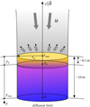 |
Fig. 1. Schematic depiction of the model describing the accretion at low Ṁ onto the polar cap of a magnetized neutron star. The polar cap is an emitting layer of an atmosphere with the total column density ymax (corresponding to the total geometrical depth zmax ∼ 10 m) and radius r0. The characteristic stopping length is denoted z0 (geometrical scale) and y0 (column density scale). |
As the atmosphere is in hydrostatic equilibrium, we can compute its density from the known temperature profile, that is, from the energy balance in the atmosphere. We do not perform a detailed computation of the actual energy loss rate through the atmosphere, dE/dy, but adopt a modified version of the approach used by ZS69 which ensures the continuity of the heating function throughout the atmosphere. We leave a deeper discussion of the energy loss rate for Sect. 5.2.
In the volume above y0, where the protons are decelerated, the conditions are likely sufficient to permit the collisional excitation of electrons into higher Landau levels. We parameterize this complex process by assuming that a fraction of the accreted energy, fcyc, goes into nonthermal collisional excitation of electrons, while the remaining fraction, 1 − fcyc, directly heats the atmospheric plasma.
The main cooling processes in the atmosphere are free–free emission and Compton cooling. Similar to ZS69 (their Eq. (1.3)), we parameterize the cooling rate for free–free processes as
and the cooling rate due to Compton scattering as
where k is the Boltzmann constant, σT is the Thomson scattering cross section, c is the speed of light, mp and me are proton and electron rest masses, respectively, and ϵ is the y-dependent radiation energy density. The last terms in Eqs. (2) and (3) account for the inverse processes, that is, free–free absorption and inverse Compton scattering. In this way, heating by free–free absorption and inverse Compton scattering is included in the cooling rates. The effective radiation temperatures T′ and T″ for both processes are taken to be equal to the photon temperature, Tph = (ϵ/ar)1/4, where ar is the radiation density constant. In this paper, when we discuss free–free processes (absorption and emission), we mean only thermal free–free processes, omitting the word “thermal” in the following.
The energy balance equation for each spatial layer of the atmosphere is thus given by
where the “effective flux” is
and where the term Feff/y0 is related to the radiative energy flux divergence, ∇ ⋅ F, representing the constant energy release per unit mass. To ensure continuity of the atmospheric profiles, which is required by the numerical scheme for the radiative transfer calculation, contrary to ZS69 we choose the heating to be characterized by an exponential cutoff instead of Eq. (4),
This modification has almost no effect on the obtained solution, except for smoothing the transition region near y0.
In this part of the modeling, we simplify the model for the radiative transfer by using the diffusion approximation for the radiant energy density, ϵ(y),
where 𝜘T = σT/mp is the opacity of a fully ionized hydrogen plasma due to Thomson scattering, and F(y) is the flux given by the formula
Choosing the Marshak boundary condition, that is, imposing flux continuity by setting  , we can write the solution of Eqs. (7) and (8) as
where
Finally, hydrostatic equilibrium yields the density distribution
where vff is the free-fall velocity and  is the density of the falling accretion flow at the upper boundary of the atmosphere.
We obtain the structure of the atmosphere by expressing the density as a function of the temperature using Eq. (11) and substituting it into Eq. (6). The temperature can then be easily calculated by using a root-finding algorithm, Newton’s method in our case. However, we emphasize that because of Eq. (6) this approach requires us to assume a value for the stopping length of the protons, y0. This quantity is not a free parameter of the model and we describe our choice of y0 in Sect. 2.5, as this assumption is closely related to our solution of the radiative transfer equation (Sect. 2.4).
2.3. Polarization and opacities
Before we describe the transport of the radiation through the atmosphere (Sect. 2.4), we first need to discuss how the radiation and photon–electron interactions are affected by the strong magnetic field. In this section, we address Compton scattering and free–free absorption in the vicinity of the neutron star (magnetic Compton scattering and magnetic free–free absorption), as these are the most relevant processes to be considered here.
The magnetized plasma of the neutron star atmosphere is an anisotropic and birefringent medium. It has a strong influence on the polarization properties of photons, because the interaction between the plasma and the radiation strongly depends on the frequency and direction of the photon propagation. Moreover, in strong magnetic fields, the effect of vacuum polarization becomes significant (see Adler 1971; Gnedin et al. 1978; Meszaros & Ventura 1978, 1979, and Lai 2001 for a review). For the conditions in the accretion columns of X-ray pulsars, this effect can become dominant over plasma effects. Wang et al. (1988) suggested characterizing the relative importance of plasma and vacuum effects by the ratio of the parameters w = (ωpe/ω)2 and δV = (1/45π)α(B/Bc)2,
where
is the plasma frequency, ω is the frequency of the electromagnetic wave propagating in the medium, α is the fine structure constant, and  is the critical magnetic field in the quantum-electrodynamical Schwinger limit. For w/δV < 1, the wave propagation is mainly affected by vacuum polarization. Conversely, when w/δV > 1, the effects of magnetized plasma play a major role. Finally, if w/δV ≈ 1, both plasma and vacuum effects have to be taken into account.
The radiation propagates in the form of two polarization normal modes. These are defined by the direction of the electrical vector of the radiation, e, in relation to the plane formed by the wave vector of the photon, k, and the magnetic field vector, B. In the ordinary mode (hereafter also referred to as “mode 2”), e oscillates in the (k, B) plane, while in the extraordinary mode (“mode 1”), e ⊥ (k,B).
We mentioned that in the presence of strong magnetic fields, because of the quantization of the electron motion perpendicular to the magnetic field on Landau levels, photon–electron interactions such as Compton scattering and free–free absorption become resonant processes. Moreover, these processes proceed differently for each of the polarization modes. The scattering and absorption cross sections of both modes differ dramatically in magnitude, especially in the soft X-ray range, and are strongly energy dependent, which has consequences for the formation of the continuum as discussed below.
Expressions for the cross sections for scattering and free–free absorption have been obtained by various authors using different approximations as well as different photon polarization modes, such as pure plasma, pure vacuum, or plasma+vacuum modes (see, e.g., Ventura 1979; Kirk & Meszaros 1980; Nagel 1981; Daugherty & Harding 1986; Bussard et al. 1986; Mushtukov et al. 2016; Sina 1996). Here, we consider one-photon Compton scattering, following the quantum mechanical derivations for differential and total scattering cross sections given by Nagel (1981). This derivation neglects the electron spin and assumes that the initial and final electron occupies the lowest Landau level, but takes into account thermal electron motion. Thus, these cross sections are appropriate for a hot, nonrelativistic plasma with kTe ≪ mec2.
The probability that a photon with initial energy E and polarization vector e, which propagates in the direction k, will have the characteristics E′, k′, and e′ after the scattering event is given by the differential cross section,
where re is the classical electron radius, dΩ = sin θdθdϕ is the solid angle element, with the azimuthal angle, ϕ, and the angle θ between vectors k and B, f(p) is the nonrelativistic Maxwell distribution for the electron momentum p, and Π is the scattering amplitude (see Eq. (5) of Nagel 1981). The δ function expresses conservation of energy in the scattering event, with p and p′ denoting the initial and final momentum of the electron, respectively. From the optical theorem the total cross section is then
where the matrix elements of the scattering amplitude,  , are averaged over the Maxwellian distribution.
We assume pseudo-local thermodynamic equilibrium and treat cyclotron absorption and reemission as scattering, assuming that the collisional de-excitation rate is lower than the radiative decay rate, consistent with our atmosphere model and the classical approach of Nagel (1980), Meszaros & Nagel (1985a), and Alexander et al. (1989). Under these assumptions, the thermal production rate of photons is given by j = αffB(Te), where B(Te) is the Planck function of the local electron temperature and where the magnetic free–free absorption coefficient, αff, includes the continuum and the resonant part due to cyclotron processes (see, e.g., Eq. (7) of Meszaros & Nagel 1985a).
Although the Nagel (1981) cross sections are given for plasma normal modes, they allow easy replacement of the polarization vectors with vacuum ones (see, e.g., Eq. (14)). For the photon energy range used in the calculations and throughout most of the atmosphere, we find with Eq. (12) that the atmosphere is dominated by vacuum effects. In the following, we therefore use the pure vacuum normal modes to describe the photon polarization state, as given by Wang et al. (1988, their Eqs. (12)a–f). This approach results in substantial acceleration of the computations. The other reason to avoid mixed plasma and vacuum normal modes is the ambiguity of the definition of the modes, as well as the fact that they become nonorthogonal when both vacuum and plasma effects are taken into account (Soffel et al. 1983). This ambiguity would require a more careful investigation (Ho & Lai 2003) and is left for a future development of the model.
To illustrate the behavior of the vacuum cross sections, in Fig. 2 we show the magnetic Compton scattering and magnetic free–free absorption cross sections for ordinary and extraordinary modes for two different electron temperatures, Te, and electron number densities, ne, choosing values that are typical for the atmospheric conditions relevant to the present study.
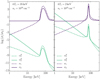 |
Fig. 2. Total cross section for magnetic Compton scattering (purple lines) and the free–free absorption coefficient (cyan lines) for the ordinary (solid) and extraordinary (dashed) polarization mode, taking into account vacuum polarization. Left: coefficients for a tenuous and hot plasma with ne = 1020 cm−3 and kTe = 35 keV, as expected for the upper, overheated layers of the atmosphere. Right: same but for cold and dense plasma with ne = 1025 cm−3 and kTe = 2 keV, corresponding to the bottom part of the atmosphere. The cyclotron line energy is Ecyc = 75 keV and the incident photon has a direction of θ = 60° with respect to the magnetic field, for both cases. |
2.4. Polarized radiative transfer
To describe the propagation of the radiation field through the atmosphere, we need to solve the radiative transfer equation. In this section, we discuss the transfer equation (taking into account the azimuthal symmetry of the task), the boundary conditions of the radiative transfer, and its numerical solution.
2.4.1. Transfer equation
In the case of the emitting region considered here, we can simplify the treatment of radiative transfer by assuming that the atmosphere is a semi-infinite, plane-parallel slab. For such a medium, we can write two equations that govern the radiative transfer in the outgoing and incoming directions,
where μ = cos θ is restricted to the half-range [0, 1], I± = I(E, ±μ,z) is the specific intensity, κ = σ + αff is the total opacity, and S is a source function.
By introducing symmetric and anti-symmetric averages of the specific intensity,
Feautrier (1964) suggested an approach that allows the radiative transfer equation to be presented as a second-order differential equation. Here, u and v are the analogs of zero- and first-order moments of the specific intensity, respectively. By adding and subtracting two equations of Eq. (16), we obtain

We can now obtain a second-order equation by expressing v in terms of u from Eq. (18b) and substituting it to Eq. (18a), which yields
In our case, the source function is given by
where the integrals represent electron scattering with partial energy and angular redistribution, with u′ = u(E′,μ′, z), and where we take into account the azimuthal symmetry of the problem. The second term describes a contribution from thermal absorption and emission with  being the equilibrium spectrum, which is Planckian with the local electron temperature. The source of nonthermal cyclotron emission at each layer of the atmosphere, Scyc, is given by
where the profile VD is determined by the Doppler broadening
with
We note that Eq. (19), together with Eq. (20), does not include stimulated processes directly (the stimulated scattering term is omitted), such that the problem is linear. However, ignoring stimulated scattering for optically thick plasma can lead to a significant excess of photons (> 50%) at high energies (Alexander et al. 1989). Meszaros et al. (1989) introduced a procedure that provides a compromise; it allows the stimulated scattering to be treated while avoiding the nonlinear problem by assuming an artificial detailed balance relation,
In equilibrium, this expression leads again to a Planckian photon spectrum. It fully reproduces the low-energy part of the spectrum obtained by solving the nonlinear problem and slightly underestimates the high-energy photon flux while keeping the same spectral shape (see Figs. 2 and 3 of Alexander et al. 1989, for a direct comparison with the nonlinear problem).
We next consider polarization effects. These require us to separate the radiation field into the ordinary and extraordinary modes, which are coupled through the scattering integral. In order to remain consistent with the description of the atmospheric structure, we rewrite the transfer equation in terms of the column density y, by taking into account that dy = −ρdz, as
where the subscript p = 1 for the extraordinary mode and p = 2 for the ordinary mode, up = up(E, μ, y), the opacity  , and the factor
  occurs from the separation of the two modes.
2.4.2. Boundary conditions
Finally, in order to solve Eq. (25), we need to specify the boundary conditions at the top of the atmosphere, y = 0, (“upper” boundary) and at y = ymax (“lower” boundary). At the upper boundary we assume that there is no external illumination of the slab, I−(0) = 0. In this case, from Eqs. (17a) and (17b) we find u(0) = v(0) and Eq. (18b) yields
The assumption of free photons emerging from the upper boundary is consistent with the physical picture of a low accretion rate, where the effects of the radiative transport in the moving plasma above the polar cap can be ignored.
At the lower boundary of the atmosphere, at high optical depths corresponding to the chosen ymax = 103 g cm−2 (and high densities, as shown in Sect. 3.1), the radiation field can be treated in the diffusion approximation, i.e., I(ymax) = B(ymax)+μ(κ−1|∂B/∂y|)ymax (see, e.g, Chap. 2 of Mihalas 1978). As the mean intensity u(ymax) = B(ymax), from Eqs. (17a) and (17b) we obtain v(ymax) = μ(κ−1|∂B/∂y|)ymax. In our case, Eq. (6) leads to the existence of an extended cold isothermal layer below y0 (see Sect. 3.1), and therefore Eq. (18b) yields

These boundary conditions together provide a self-emitting slab, where free–free emission, including both continuum and resonant parts of the coefficient, and non-thermal cyclotron emission are the only sources of photons.
2.4.3. Numerical solution
We model the radiative transfer by discretizing Eq. (25) for each polarization mode using an appropriate angular {μ}, energy {E}, and column density (“spatial”) {y} grid. We then write a matrix equation for each y-layer and solve the system of matrix equations using a tridiagonal matrix algorithm. This approach to solving the transfer equation for atmospheres with predefined temperature and density profiles is known as the Feautrier method (Feautrier 1964). The method is efficient even for optically thick atmospheres and allows for partial angular and energy redistribution. The application of the method to the polarized radiation in magnetized atmospheres was described by Nagel (1981), Meszaros & Nagel (1985a; see also Chap. 6 of Mihalas 1978, for the classical formulation). We follow the prescriptions of Auer (1967) to improve the boundary conditions by performing a Tailor series expansion away from the boundary, including terms up to the second order. Our code for the radiative transfer simulation, FINRAD, is written in Python 3 and is based on sparse matrices. It was extensively tested using known analytical and numerical solutions for scattering atmospheres and the well-known transfer code XILLVER for reflection from accretion disks (J. A. Garcia, priv. comm.) Some examples of this code verification are presented in Appendix A.
2.5. Complete simulation
In order to determine the structure of the atmosphere and then use it to solve the radiative transfer equation, we first need to obtain an estimate of the stopping length of protons, y0. The detailed modeling of the proton stopping at the level of for example Kirk & Galloway (1982) or Miller et al. (1987) is outside the scope of this paper. Instead, we iteratively find y0 for each given set of the parameters, {Ṁ, r0, Ecyc, fcyc}, by requiring that energy is conserved inside the emitting region. Specifically, for a chosen Ṁ, we require that all kinetic energy of the accretion flow is converted to the radiation emerging from the atmosphere,
We restrict the calculated bolometric flux by setting
where F1 and F2 are the specific fluxes of the extraordinary and the ordinary mode, respectively.
In order to obtain a self-consistent model of the atmosphere, for each set of parameters {Ṁ, r0, Ecyc, fcyc} we choose an initial value for y0 (usually, y0 = 6–9 g cm−2), calculate the atmospheric structure based on the discussion in Sect. 2.2, and then solve the radiative transport as described in Sect. 2.4 to obtain the flux. We then compare the resulting luminosity of the slab, Lnum, to Lacc and, if necessary, adjust y0 iteratively until energy conservation is achieved at better than 10% tolerance, that is, until |Lnum − Lacc|/Lacc < 0.1. The total process of the simulation is illustrated in Fig. 3.
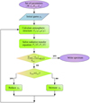 |
Fig. 3. Flowchart of the complete numerical solution. |
For the discretization of the spatial scale, we use a logarithmic grid within the range y = 10−3 − 103 g cm−2. We continue our grid to such high column densities (compared to y0) to ensure that the medium has a sufficiently high optical depth for both polarization modes over a wide energy range. Angular discretization is performed according to the 8-point double-Gauss formula for μ given by the roots of the Legendre polynomial in the range [0, 1] (see Sykes 1951; Mihalas 1978, Chap. 3). The energy grid requires more care, as it is necessary to ensure a fine grid around the cyclotron resonance while the grid in the continuum can be coarser. At the same time, however, the steps in the energy grid should not change abruptly as this can lead to instabilities in the numerical scheme and also strongly affects the redistribution in energy. Our compromise solution is to use a nonuniform grid generator where the points condense gradually towards the so-called target, which in our case is the cyclotron resonance. Here, we apply the generator by Tavella & Randall (2000), which gives the grid points
where
and where the parameter ζ determines the uniformity of the grid. In our calculations, we choose ζ = 0.3 and set Emin = 0.8 keV, Emax = 250 keV, with a total of 300 points on the energy grid.
3. Spectral formation and atmospheric structure
In this section, we describe the obtained atmospheric structure, the formation of the emergent radiation field, and its spectral shape. We base our discussion on a parametric study of a set of 144 spectra in which we varied the mass-accretion rate, polar cap radius, magnetic field, and the fraction of accretion energy going into nonthermal collisional excitation of electrons over the following parameter ranges: Ṁ = [4−16] × 1013 g s−1, r0 = [80−140] m, Ecyc = [50−80] keV, fcyc = [0−0.4]. The neutron star mass and radius are fixed to 1.4 M⊙ and 12 km, respectively.
3.1. Atmospheric structure
We start our discussion with a description of the internal structure of the atmosphere, which to a large extent determines the shape of the emergent spectrum. Figure 4 (right) shows the electron temperature and density distribution along the vertical axis in the atmosphere for a typical set of parameters. The atmosphere has two principal parts determined by y0. In the upper part, where y < y0, the heating by accreted matter significantly affects the energy balance (Eq. (6)). The temperature of this region mainly depends on y0 and reaches values of 30−40 keV. Media with shorter y0 have a higher temperature as the accretion energy dissipates in a smaller volume. In the dense lower part of the atmosphere, only the balance of free–free processes and Compton scattering determines the low equilibrium temperature (∼2 keV). A constant level of the local electron temperature is reached soon after y0 and depends mainly on the ratio  , which controls the properties of the falling flux at the upper border of the atmosphere through the continuity equation. We also emphasize which parts of the atmosphere play a major role in the formation of individual spectral components. We focus on this in the following sections.
 |
Fig. 4. Left: emerging spectrum in two polarization modes. Solid lines describe the total flux, dotted lines extraordinary, and dashed lines ordinary photons. Right: atmospheric structure: electron temperature (solid) and number density (dash-dotted). The major spectral components and associated formation regions are indicated in both panels. |
In addition to the column density, Fig. 4 (right) shows the scales for optical and geometrical depths in the atmosphere. We emphasize that even though the total column density ymax is high, the atmosphere remains a geometrically thin layer of only ∼10 m. This justifies our assumption about a constant magnetic field along the vertical direction inside the atmosphere and allows us to estimate the effect of gravitational redshift on the emitted spectrum (see, e.g., Sect. 4). In addition, it validates the choice of one-dimensional treatment for the radiative transfer, as the surface area of the sidewall of the atmospheric slab, Asw = 2πzmaxr0, is much smaller than the polar cap area,  . The simple estimate on the corresponding luminosities yields Lsw/Ltop < 2zmaxr0 ≪ 1. Thus, the radiation flux through the sides can be neglected. The escape of photons from the sidewall is still by no means free and is determined by the radiant thermal conductivity of the magnetized plasma.
3.2. Formation of the emitted spectrum
We can now discuss the spectral formation in the atmosphere with pre-calculated structure as a result of photon–electron interactions in a highly magnetized medium in detail. We first investigate the formation of the spectrum in the absence of nonthermal collisional excitations in the atmosphere, i.e., fcyc = 0. This case corresponds to a very strong magnetic field where the energy of the flow is insufficient to excite the electrons even to the first Landau level. This approach allows us to illustrate the details of the second hump origination.
A typical energy flux (times energy) for low mass-accretion rates onto a magnetized neutron star from the polcap model is shown in Fig. 4 (left), corresponding to the atmospheric structure from Fig. 4 (right). The overall emerging spectrum has two dominant spectral components: a softer, thermal hump and a high-energy, second hump characterized by a cyclotron line.
We can understand the formation of the spectrum by studying how the photon density,
changes throughout the atmosphere in our model. The mean intensity J can be found at each internal spatial layer by calculating the quadrature over angles, Jp(E, y) = ∑wμup(E, μ, y), where wμ are the weights given by the double-Gauss formula. The top part of Fig. 5 shows the evolution of the photon density spectrum inside the atmosphere. Starting at the bottom of the slab, at the highest optical depth, τT ≈ 4 × 10², the free–free absorption dominates opacities for both modes (see the right-hand side of Fig. 2, displaying the scattering cross sections for similar conditions) and the radiation field is at local thermodynamic equilibrium. The photon spectrum is Planckian corresponding to the local electron temperature kTe = 2 keV. At higher but still optically thick layers of the slab, one can see the effect of Compton up-scattering and the formation of the cyclotron scattering feature. As the scattering coefficient in the line core is very high, the photons are mainly scattered out of the core, forming pronounced shoulders to the line on top of the comptonized continuum. Closer to τT ≈ 1, the temperature profile is affected by the heating of the slab by accreted matter. This results in more efficient Compton up-scattering of softer photons and further diffusion of the photons away from the line core, which together with the significant temperature gradient fills up the feature, making it almost completely disappear. At small optical depths, τT ≲ 10−2, the continuum is not further affected by scattering, except for the region near the cyclotron energy. As the upper part of the atmosphere has a very high electron temperature, the resulting cyclotron line is very broad. We find that its width can be well estimated by assuming pure Doppler broadening (Meszaros & Nagel 1985a),
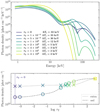 |
Fig. 5. Top: photon density at different optical depths of the neutron star atmosphere, τT, summed over polarization modes. The set of model parameters is the same as in Fig. 4. Bottom: photon density integrated over photon energies in each polarization mode. Markers correspond to the lines of a similar color in the top panel; circles indicate ordinary and crosses extraordinary photons. |
In the case discussed here, kTe = 33 keV, Ecyc = 70 keV, and ⟨cos θ⟩ = 2/π result in EFWHM ≈ 27 keV, in agreement with the line width from our simulation.
The bottom panel of Fig. 5 shows the energy-integrated photon density profile inside the atmosphere. Deep in the atmosphere, both photon modes are thermal and mixed. As a result, radiation is unpolarized. The extraordinary mode saturates to the equilibrium value much deeper in the atmosphere because of the much lower opacity. Because the mean free path, λ, scales as λ ∝ σ−1, at low energies extraordinary photons have a much longer mean free path than ordinary ones (see Fig. 2). For this reason, soft extraordinary photons can leave the medium from deeper layers of the atmosphere, and the radiation becomes polarized. The density of extraordinary photons is additionally increased by mode conversion during scattering events. Once an ordinary photon has changed its polarization during scattering, it can leave the medium. As a result, the spectrum of the emergent radiation is dominated by soft extraordinary photons. The high-energy photons and the ordinary mode are trapped in the atmosphere longer by the resonant scattering. For both polarizations, photon densities decrease towards the top of the atmosphere, reaching the limiting values at an optical depth comparable with their mean free path. We note that these conclusions are in agreement with the results of Meszaros & Nagel (1985b) for a deep optically thick atmosphere.
In summary, the high-energy component is mainly produced by resonant magnetic Comptonization in the heated nonisothermal part of the atmosphere, and then modified by the formation of the cyclotron line in the optically thin layers. Our polarization-dependent computations also show that the fluxes of ordinary and extraordinary photons emerging from the atmosphere at the high-energy component are very similar to each other. This is caused by the large cross sections around the cyclotron resonance for both modes. However, more actively comptonized ordinary photons dominate in the line core.
In contrast, the low-energy component is mainly formed by extraordinary photons. As extraordinary photons can escape from deeper layers of the atmosphere, the soft thermal emission in this mode is not modified dramatically by scattering. For the ordinary photons, on the other hand, the soft thermal emission is significantly changed by Compton up-scatterings. Here, we see a flattened spectrum in the low-energy part of the ordinary mode, which results from saturated Comptonization, in agreement with previous results for high optical depth in magnetic (Meszaros & Nagel 1985a) and nonmagnetic (Sunyaev & Titarchuk 1980) atmospheres. Considering this and the dominant contribution of the extraordinary mode to the low-energy part of the spectrum, we can therefore expect the outgoing radiation to have a high degree of polarization. The distinguished contribution of the ordinary and extraordinary photons to the soft and hard energy band of the emerging spectrum is also well known from the studies of Ceccobello et al. (2014) and Lyubarskii (1988a,b).
3.3. Parameter dependency of the emitted spectrum
We now turn to studying the effects of the model parameters on the photon spectra emerging from the neutron star atmosphere. We choose a baseline model with parameters Ṁ = 1.6 × 10¹⁴ g s−1, Ecyc = 70 keV, r0 = 140 m, and fcyc = 0. The energy flux times area is always shown for this model in purple in Figs. 6a–d (left), with the corresponding atmospheric profiles on the right. We then vary each parameter individually and show the spectra and the atmospheres relative to this model. By decreasing the mass-accretion rate compared to our baseline model (Fig. 6a), we obtain a lower bottom temperature and, consequently, a weaker and softer thermal hump. At a lower accretion rate, our iterative solution for the atmosphere reaches the energy conservation (Eq. (29)) at a higher y0. Consequently, the volume in which most of the accretion energy is released increases. This leads to a lower temperature also in the entire upper part of the atmosphere, and, accordingly, to a less active formation of the second hump, by reducing the Compton-y parameter,
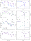 |
Fig. 6. Dependency of the emerging spectra (left column) and atmospheric structure (right column) on the model parameters. The spectra are shown in energy flux times polar cap area, i.e., in luminosity units, for both polarization modes. From top to bottom, we show how the spectral shape and the structure of the atmosphere depend on the mass-accretion rate, Ṁ (a), the polar cap radius, r0 (b), the cyclotron energy, Ecyc (c), and the fraction of the accretion energy going into nonthermal collisional excitations, fcyc. The same baseline model is shown in purple in all panels. See text for further discussion. |
for a magnetized plasma. We note that Eq. (34) is applicable only to the continuum formation and should be understood only in the sense of dependence on electron temperature in case of partial energy redistribution, which is responsible for the second hump formation. A decrease in the polar radius (Fig. 6b) leads to the opposite effect on the atmosphere, as compared to a decrease in the mass-accretion rate because the volume of the entire energy release decreases. Thus, the temperature rises throughout the atmosphere and the thermal hump becomes much harder. However, as we show spectra in energy flux times area units, it is clear that the luminosity is lower for the model with a smaller polar radius. Both a decrease in r0 and an increase in Ṁ, i.e., increase in flux density, ρ0vff = Ṁ/A, leads to the higher stopping length.
Figure 6c shows that reducing the cyclotron energy, that is, the surface magnetic field, to 50 keV does not affect the thermal hump. Even though the temperature of the upper part of the atmosphere decreases, the strength of the second hump is not reduced, although it is shifted to lower energies. The formation of this spectral component directly depends on the cyclotron energy and the temperature of the upper atmosphere. As we reduced the cyclotron energy much more than the upper temperature, we left room for more efficient energy redistribution near the cyclotron resonance, resulting in strong wings and a deep line. However, it is important to mention that the width of the line only appears to be bigger than it is at higher cyclotron energy because of the logarithmic energy scale.
Finally, we allow nonthermal collisional excitations during the plasma braking in the atmosphere (Fig. 6d). We increase the parameter fcyc to 0.4, and so now 40% of the accreted energy goes into collisional excitations of the ambient electrons, whereas the rest contributes to heating. This change does not affect the stopping length, y0, as we just redistribute energy sources. For the atmospheric profile, it mainly lowers the bottom temperature, softening the thermal hump. Simultaneously, we see a rise in the second hump, as the shoulders become stronger and the cyclotron line more shallow. Thus, the main effect of adding a source of nonthermal cyclotron photons is a change in the ratio of the thermal and the high-energy humps while simultaneously reducing the line depth.
4. Application to data: fitting GX 304−1 with polcap
The spectral shapes discussed in Sect. 3 are in qualitative agreement with the spectral shapes seen from accreting neutron stars in the low Ṁ limit. However, only fitting the model to real data will give a clear idea of its applicability. To that end, we apply the polcap model to analyze deep observations of the Be X-ray binary GX 304−1 made with NuSTAR and Swift/XRT.
GX 304−1 was discovered in October 1967 during a balloon flight from Mildura, Australia (Lewin et al. 1968a,b), and later by McClintock et al. (1971) in 1970. Observations with the Small Astronomy Satellite 3 (SAS 3) in February 1977 revealed regular X-ray pulsations with a period of about 272 s (McClintock et al. 1977). GX 304−1 consists of a highly magnetized neutron star and the main sequence fast-rotating Be-star V850 Cen. The system is located at a distance of about 2 kpc (Parkes et al. 1980; Rouco Escorial et al. 2018). At the time of discovery, the source showed the typical behavior of accreting neutron stars in Be-systems, with regular type I outbursts at an orbital period of 132.5 d, which are associated with the periastron passages of the neutron star through the excretion disk of the Be star donor (Priedhorsky & Terrell 1983). GX 304−1 showed two periods of regular activity. The first one lasted from the moment of the discovery until 1980, when its flux dropped to quiescence (Pietsch et al. 1986), followed by an “off” state lasting 28 yr.
Renewed activity of GX 304−1 was found with INTEGRAL in 2008 (Manousakis et al. 2008), and the source stayed active until mid-2013. During this time, using data from the Rossi X-ray Timing Explorer (RXTE) and Suzaku, Yamamoto et al. (2011) discovered a CRSF with a centroid energy of ∼54 keV. A later analysis showed that the CRSF is positively correlated with source luminosity (Klochkov et al. 2012; Malacaria et al. 2015). Malacaria et al. (2015) found the CRSF detectable at all rotation phase bins and obtained a maximum centroid energy of 62 keV, corresponding to a magnetic field strength of 6.9 × 10¹² G. Jaisawal et al. (2016) discovered a significant variation of the cyclotron line parameters with rotational phase.
Malacaria et al. (2017) showed that the irregular activity of GX 304−1 is closely related to the circumstellar disk evolution. During the outbursts, when GX 304−1 has a typical luminosity of 1036 − 1037 erg s−1, the spectra are well described by a cutoff power law (Yamamoto et al. 2011; Jaisawal et al. 2016). Kühnel et al. (2017a) showed that intervals of increased absorption column during this time are compatible with an inclined Be disk, consistent also with the model for changes in the geometry of the large-scale accretion flow (Postnov et al. 2015b). Rothschild et al. (2017) suggested that the spectral shape and positive correlation of the CRSF with luminosity can be explained assuming the accretion flow is in the collisionless shock-braking regime. In the quiescent state, however, a recent NuSTAR observation shows the source to have a bimodal spectral shape with humps around 5 keV and 40 keV and comparable energy fluxes (Tsygankov et al. 2019a), resembling the spectral shapes discussed in Sect. 3. This makes GX 304−1 an ideal candidate to test the polcap model on observational data.
We used a low-luminosity NuSTAR observation of GX 304−1 taken on 2018 June 3 (ObsID 90401326002), which is complemented by a contemporaneous Swift/XRT observation (ObsID 00088780001). We processed the NuSTAR data with NUSTARDAS pipeline version 2.0.0 with CalDB version 20201101 under HEASoft V6.28. Source and background regions for both NuSTAR focal plane modules (FPMs) are circles of 30″ radius centered on the source and outside the point spread function wings, respectively. We reprocessed the Swift/XRT data with xrtpipeline version 0.13.5. Source and background spectra were extracted using XSELECT version 2.4 for a circular source region of 20″ radius and an annulus background region with radii of 80″ and 120″. We use ISIS v. 1.6.2 for our spectral analysis (Houck & Denicola 2000). We applied optimal binning following the approach of Kaastra & Bleeker (2016) and used Cash statistics (Cash 1979) for spectral fitting. As the observation was performed during a deep quiescent state, we find the high-energy band to be strongly background dominated above ∼35 keV. Therefore, we restrict the energy range used for spectral fitting to 1–6 keV and 4–35 keV for Swift/XRT and NuSTAR, respectively.
To compare the polcap model with the data, we use the results from the parametric study described in Sect. 3 to generate an additive table model that is compatible with XSPEC and ISIS. Thus, the table model contains 144 spectra, between which interpolation is possible. To obtain the flux on the detector, we multiply the flux in the neutron star rest frame by the factor  , for a distance D = 2 kpc. We note that this approach implies symmetric accretion onto two poles and isotropic emission. Models in which these very simplifying assumptions are relaxed will be presented in a subsequent paper. We fix the gravitational redshift to z = 0.24, as is appropriate for the surface of a neutron star with MNS = 1.4 M⊙ and R = 12 km. Finally, we account for photoelectric absorption in the interstellar medium using the tbnew model with the cross sections by Verner et al. (1996) and abundances by Wilms et al. (2000).
In XSPEC-like notation, the complete model used in our spectral fits is

where detconst accounts for differences in flux calibration between the FPMA and FPMB detectors onboard NuSTAR, as well as the difference between FPMA and Swift/XRT calibration. We note that we explicitly do not re-scale our model during the fit in order to ensure that we reproduce not only the spectral shape but also the absolute value of the energy flux. Figure 7 shows the unfolded phase-averaged spectrum and the best-fit model, the parameters and statistics for which are presented in Table 1. Figure 8 provides confidence plots to map the parameter space. The maps are calculated by stepping through the two-dimensional grid corresponding to the two parameters of the model and fitting the data at each point of the grid. The obtained statistic is then compared to the best-fit one (Table 1). Contours for all parameters show an absence of degeneracies.
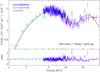 |
Fig. 7. Unfolded spectrum of the low-luminosity observation of GX 304−1 in EF(E) with the best-fit model (solid black line) for NuSTAR FPMA (blue), FPMB (violet), and Swift/XRT (cyan). For clarity we rebinned the spectra with larger bins for plotting than the ones used for the fit (top). Ratio for the best-fit model (bottom). |
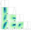 |
Fig. 8. Parameter probabilities for the polcap model applied to the low-luminosity observation of GX 304−1. Correlations for different parameters are shown in color as two-dimensional confidence maps, where dotted, dashed, and solid contours correspond to the 99%, 90%, and 68% confidence regions, respectively. Here “ΔC-Stat” represents the statistic change compared to the best fit. Side panels on the right show the one-dimensional parameter probabilities. |
Overall, the spectrum shows the double-hump shape discussed above. The high-energy excess in the spectrum is described by the left-hand part of the second hump; that is, the red wing of the cyclotron line formed in the hot nonhomogeneous atmosphere due to resonance Compton scattering.
The mass-accretion rate from the best-fit model is ∼6.4 × 10¹³ g s−1 and cyclotron energy is ∼58 keV, which corresponds to a surface magnetic field B0 = 5 × 10¹² G. The fundamental cyclotron line, in this case, would be observed at ∼58 keV/(1 + z) ≈ 47 keV. This energy agrees with previous results, although in this case we rather expect to see higher cyclotron line energy, breaking the positive correlation of the CRSF with luminosity discussed by Rothschild et al. (2017, and references therein), as emission comes directly from the surface of the neutron star. However, the cyclotron line energy range itself is not available for the analysis in this observation as the data above ∼35 keV are dominated by background. The Ecyc parameter in this case is mainly affected by the position of the left-hand part of the second hump, which is not well constrained. In addition, the line position depends on the angle under which the emission region is observed. Thus, by using the spectrum averaged over the angles and avoiding the relativistic ray tracing from the neutron star surface, we lose some information about the line centroid energy. We will analyze this in detail in our future paper on a pulse-resolved extension of the polcap model (Sokolova-Lapa et al., in prep., hereafter Paper II). The polar cap radius of ∼130 m is close to the estimate for a hot spot area for a dipole field (Lamb et al. 1973),
where  is the Alfvén radius, with dipole moment
  and ξ = 1. In reality, the coefficient ξ is close to unity, but its exact value depends on a screening factor originating from currents induced on the surface of an accretion disk, and on the magnetic pitch at the inner edge of the disk (Wang 1996). The fcyc parameter from the best-fit has a value of ∼0.23, which means 23% of the energy of the accretion flow goes into nonthermal excitations of Landau levels. As mentioned above, this parameter mainly affects the relative strength of the two spectral components and can be influenced by the fact that the high-energy component is not well constrained. The total luminosity under the assumptions stated above is L = 1.2 × 1034 erg s−1.
5. Summary, discussion, and conclusions
5.1. Summary
In the present paper we discuss our model of accretion at low Ṁ onto magnetized neutron stars. Despite the obvious simplifications in our approach, we obtain an internally consistent structure of the atmosphere and the radiation field. This allows us to understand, although partly in a parametric way, the physics of accretion at low Ṁ and how these parameters influence the emitted spectrum and its polarization.
We first show that the atmosphere has a two-zone structure consisting of a very hot layer, which is mainly cooled by Compton scattering, and a colder interior. Using angle-dependent, polarized radiative transfer computations, we showed that this structure leads to a spectral energy distribution that is characterized by two humps. The most important results of our detailed radiative transfer are the following:
-
The physical origin of the two-humped X-ray spectral shape is the strong polarization and temperature dependency of the Compton scattering cross section.
-
The lower energy, thermal hump is mainly formed by the extraordinary photons that originate in the deep layers of the atmosphere.
-
The harder, second hump is due to resonant magnetic Comptonization in an atmospheric layer with a strong temperature gradient, and is modified by the cyclotron line in the upmost hot layer.
-
A fraction of the accretion energy is used to excite atmospheric electrons into higher Landau levels, which affects the relative luminosity of the two spectral components.
The formation of a high-energy excess by Comptonization in the overheated part of the atmosphere with optical depth around unity is well known for nonmagnetic plasmas in neutron star low-mass X-ray binaries (see, e.g., Deufel et al. 2001; Suleimanov et al. 2018) and in X-ray binaries with black holes (e.g., Sunyaev & Titarchuk 1980; Hua & Titarchuk 1995; Dove et al. 1997; Wilms et al. 2006, and references therein). For high magnetic field values (with corresponding Ecyc ≳ 40 keV) this region is also modified by the resonant nature of the scattering. We expect this process to always be present in highly magnetized atmospheres with a strong temperature gradient such as that formed in the case of Coulomb collisions. As we showed in Sect. 3, even without nonthermal collisional excitations in the atmosphere (whose contribution is highly conditional) the high-energy component in the spectra is produced by resonant magnetic Comptonization.
Our model can quantitatively explain the observational data of GX 304−1 at low luminosities. The parameters for the atmosphere that are obtained with the model appear physically reasonable, with a polar cap radius of ∼130 m, mass-accretion rate of 6.4 × 10¹³ g s−1, and cyclotron energy of 58 keV at the surface of the neutron star. The model requires about 23% of the accreted energy to go into nonthermal excitation of electrons in upper Landau levels.
These results open up various avenues for further refinement of the study of the physics of accretion onto neutron stars at low mass-accretion rates. In the following sections, we describe these avenues in more detail, starting with the general atmospheric structure in Sect. 5.2, and then discussing our expectations as to the collisional excitation of electrons as part of the process of plasma stopping in the neutron star atmosphere (Sect. 5.3). In Sect. 5.4, we address the alternative possibility of matter stopping at low mass-accretion rates, the collisionless shock. Finally, we summarize the prospects for further development of the model in Sect. 5.5.
5.2. Atmospheric structure and proton stopping
As discussed above, the atmospheric structure of our model is typical for collisionally heated atmospheres, with a hot optically thin layer near the surface and a colder deep interior. In Sect. 3.3 we show that the temperature of the overheated layer is highly dependent on the proton stopping length. In our model, y0 is obtained indirectly as a result of the iterative procedure described in Sect. 2.5. This approach, while greatly simplified, nevertheless allows for some consistency between the atmosphere and the radiation field. It also rules out the unphysical solutions and parameter values that give overly high or, conversely, unrealistically low emitting power of the atmosphere.
The real picture of plasma braking in the neutron star atmosphere is much more complicated, although it can be parameterized well in our approach. It can be divided into three main sub-problems: (i) the evolution of the distribution function of the falling protons after entering the atmosphere, (ii) the balance between heating and cooling in the atmospheric plasma and, finally, (iii) the radiation propagation in the atmosphere. These problems, which are often complex by themselves, in principle would need to be addressed in a self-consistent manner. Advanced models (e.g., Meszaros et al. 1983; Harding et al. 1984; Miller et al. 1987, 1989; Nelson et al. 1993, 1995) couple, to some degree, the proton stopping, energy balance, and radiative processes, but still contain a number of serious simplifications, especially regarding spectrum formation.
The Coulomb braking regime assumes that the incident flow gradually loses energy inside the nearly static atmosphere of the neutron star by proton–electron Coulomb collisions (with and without electron excitation to a higher Landau level). The stopping power of the plasma is also affected by the generation of the collective plasma oscillations. The energy loss of protons falling along the z-axis, resulting from both individual encounters and collective effects, is (see, e.g., Nelson et al. 1993)
where we implicitly define the Coulomb logarithms and where the term Λind includes both types of collisions, with and without excitations. Equation (37) also provides the heating rate throughout the atmosphere, which is to be used in the energy balance.
For a strong magnetic field, when only excitations up to 1–2 Landau levels are possible, the stopping power of the atmosphere is smaller than in the nonmagnetic field case. Meszaros et al. (1983) and Harding et al. (1984) found a stopping length of ∼20 g cm−2 from their stopping simulations in an inhomogeneous atmosphere for collisions with small pitch angles. Miller et al. (1989) included Coulomb collisions for arbitrary pitch angles and momentum transfer, obtaining a stopping length of ∼40 g cm−2. In this case, bremsstrahlung remains the main source of photons, although a fraction of the accretion stream energy is converted to cyclotron radiation produced by the decay of collisionally excited electrons. We discuss the effect of this process in detail in Sect. 5.3. The values of y0 found by our iterative simulations (Sect. 2.5) are lower than those obtained in the previous works on magnetic atmospheres. This behavior is a consequence of the assumed energy release profile along the z-axis of the slab (see Eq. (6)). The more detailed simulations of the Coulomb braking in the atmosphere show that although the rate of energy loss can stay nearly constant throughout a significant part of the atmosphere, it is lower than that given by our simplified expression.
We note that we use nonmagnetic coefficients to calculate the energy balance (see Eqs. (2) and (3)) in the current version of the model, and thus the magnetic field strength on the surface of the neutron star can influence the structure of the atmosphere only indirectly through its effect on y0 search in the numerical procedure. However, similar to the model used here, more complex calculations (Miller et al. 1989; Harding et al. 1984) also result in temperature profiles with a thin hot Compton cooling layer on top and a much cooler lower region, similar to the nonmagnetic case. The atmospheric profiles obtained with our model successfully mimic this self-consistent calculation for magnetic atmospheres, which suggests that our approach is adequate for studying the spectrum emerging from such atmospheres.
5.3. Collisional excitation
The contribution of nonthermal collisional excitations to the process of plasma stopping in the atmosphere of a neutron star strongly depends on the strength of the source magnetic field (the higher the field, the fewer excitations are possible) and the velocity of the accretion flow, and is difficult to assess. For this reason, we parametrize the contribution of collisional excitations to the stopping process by introducing the parameter fcyc. We then exclude this fraction of energy from the heating of the atmosphere (Eq. (4)), and directly convert it into cyclotron photons (accounting for the Doppler broadening, Eq. (21)). This approach allows us to investigate the influence of nonthermal collisional excitations on the formation of the spectrum. We found fcyc = 0.23 for the case of the low-luminosity observation of GX 304−1, which means that about 23% of the accreted energy is going into excitations of electrons to the higher Landau level. In this section, we try to assess how reasonable this number is.
If the plasma approaches the neutron star surface at free-fall velocity, vff, then the maximum Landau level to which electrons can be excited in electron–proton Coulomb collisions is
For our modeling of the spectra of GX 304−1, with assumed parameters MNS = 1.4 M⊙ and radius RNS = 12 km, and using the cyclotron energy at the surface of the neutron star, Ecyc = 58 keV, we find nmax = 1.
In detailed simulations of the proton stopping in neutron star atmospheres, Miller et al. (1989) showed that for magnetized atmospheres with nmax up to 2 and for B = 5 × 10¹² G, the fraction of the accretion energy going into collisional excitations of Landau levels is about 10% (Table 1, last column, in Miller et al. 1989). This is similar to the model of Nelson et al. (1993, 1995), which predicts a high-energy excess due to cyclotron photons as a result of the collisional excitations in the atmosphere for nmax ≫ 1. For high nmax, Nelson et al. (1993, 1995) predict a significant contribution of the collisional excitations to the stopping process. However, for low nmax = 1, 2, the results of these authors agree with those of Miller et al. (1989; see, e.g., Fig. 7 in Nelson et al. 1993). The best-fit result of our parametrized description of nonthermal collisional excitation is slightly higher than given by these simulations. This could be attributable to the fact that the high-energy component is not well constrained in the low-luminosity observation of GX 304−1, or that we ignore the energy losses in the atmosphere, for example those caused by the generation of the collective plasma oscillations, within the framework of our model. The latter can lead to a decrease in the strength of the low-energy component and result in the lower value of fcyc found by the best fit.
We conclude that for highly magnetized atmospheres and low accretion rates, Coulomb collisions without excitations remain the main mechanism of plasma braking, such that ∼80% of the accreted energy is used to heat the atmosphere.
Finally, we comment on the consequences of these estimates for observations of other sources. In Sect. 3.3 we show that while a high-energy excess in the spectra is formed in the absence of the seed cyclotron photons (fcyc = 0) by magnetic Comptonization, the real data require a contribution of photons from nonthermal collisional excitations that amounts to fcyc = 0.23 to explain the spectral energy distribution of GX 304−1. We suggest a similar mechanism for the formation of the high-energy excess of other highly magnetized sources at very low luminosities, namely resonant magnetic Comptonization in the nonhomogeneous atmosphere with a contribution of the nonthermal cyclotron emission (depending on the source magnetic field). Thus, for A 0535+262, with a slightly lower magnetic field (Ecyc = 48(1 + z) keV), following Sect. 5.3 we obtain nmax = 1–2, depending on the neutron star mass and radius. For X Persei, estimates of the magnetic field value vary. The proposed value from accretion torque models yields B ∼ 1014 G (Doroshenko et al. 2012). Assuming that the spectral formation for X Persei is similar to that for GX 304−1 and A 0535+262, as suggested by Tsygankov et al. (2019a,b), we expect the cyclotron line to be located above ∼100 keV which implies a magnetic field B ≳ 9 × 10¹² G (Mushtukov et al. 2021). Similarly, the magnetic field for GRO J1008−57 is estimated to be B ≳ 6.5 × 10¹² G, with a cyclotron line observed at 78 keV (Kühnel et al. 2017b; Bellm et al. 2014; Yamamoto et al. 2014), and a recent claim of a significantly higher energy of ∼90 keV (Ge et al. 2020). In the case of such high magnetic fields, collisional excitations in the atmosphere are barely possible. We therefore conclude that models that explain the high-energy component mainly by collisional excitations followed by cyclotron photon emission (Tsygankov et al. 2019b; Mushtukov et al. 2021) require an unreasonably high contribution of this process for the Coulomb braking regime, which is not supported by the detailed studies on collisional stopping in magnetized atmospheres.
5.4. Collisionless shock
So far we consider that Coulomb collisions in the neutron star’s nearly static atmosphere are responsible for the braking of the down-falling plasma, as suggested by ZS69 for spherical accretion and later developed by many others for nonmagnetic (see, e.g., Turolla et al. 1994; Deufel et al. 2001) and magnetic (Kirk & Galloway 1982; Miller et al. 1989, and references therein) atmospheres. We note, however, that Shapiro & Salpeter (1975) proposed an alternative scenario that also develops at low accretion rates onto a magnetized neutron star. In this scenario, a standing adiabatic shock wave forms at some distance, hs, above the surface due to rapidly grown plasma instabilities (Bykov & Krasil’Shchikov 2004). The post-shock velocity of the accretion flow is greatly reduced, vs ∼ vff/4 (Shapiro & Salpeter 1975). The matter therefore loses a significant fraction of the kinetic energy passing through the narrow transitional region. This energy release results in hot electrons behind the shock that cool down mainly by the Compton effect, similar to the upper layer of the Coulomb heated atmosphere. Bykov & Krasil’Shchikov (2004) simulated the origin of collisionless shocks for intermediate mass-accretion rates, Ṁ ∼ 1015 − 1016 g s−1.
Further studies are required to make a clear distinction between the two regimes, stopping in the atmosphere by Coulomb collisions and by passing through a collisionless shock. The important test here is the behavior of the cyclotron line with luminosity. For the case of plasma braking in the neutron star atmosphere, the line stays constant with changing mass-accretion rate because the height of the atmosphere is almost independent of this parameter. In contrast, the height of the collisional shock decreases with increasing mass-accretion rate, which can result in a shift of the line forming region to higher magnetic field values. Rothschild et al. (2017) applied this model to explain the positive correlation of the cyclotron line with luminosity in the spectra of GX 304−1 at intermediate mass-accretion rates. Similarly, Vybornov et al. (2017) studied the variability of the cyclotron line and the continuum hardness ratio with luminosity in the spectrum of Cepheus X−4 based on the collisionless shock model. However, they assumed that the emission from the aftershock region has the typical power-law spectrum. A more accurate study of the spectral formation under the assumption of a collisionless shock is required. Another possibility to distinguish between collisionless shock and Coulomb braking regimes may come from studying the pulse profiles, which are expected to be different for the case of an emitting hot spot and an accretion column.
5.5. Outlook
Despite the simplifications outlined in the previous sections, our model of accretion onto magnetized neutron stars at low Ṁ already gives a good description of the observations. However, further modeling work and analysis of observations are needed to test the model and its limitations. First of all, based on our discussion of the contribution of the collisional excitations to the spectral formation in Sect. 5.3, we argue that more careful simulations of the stopping process in the column are needed. In addition, these need to be compared with data from other highly magnetized sources at low luminous states, for example, A 0535+262, GRO J1008−57, and X Persei, in order to test the consistency of the contribution of nonthermal collisional excitations with an estimate of the source magnetic field.
A second extension of the current model would be to perform increasingly detailed simulations of the cyclotron processes. Specifically, the effect of plasma polarization on the normal modes and the relativistic effects on the scattering cross sections have to be included in the radiative transfer. Alexander et al. (1989) showed that the relativistic cyclotron line is sharper, narrower, and appears at slightly lower energies than the nonrelativistic one for the radiative transfer under the same atmospheric conditions. We assume that this might influence not only the line formation itself at the most superficial layers of the atmosphere but also the near-resonant scattering that forms a high-energy continuum. In addition, the introduction of proper modeling of stimulated scattering, rather than the approximate modeling used here, could affect the high-energy spectrum by slightly increasing the flux of the second component. The consistency of the model can furthermore be significantly improved by direct coupling of the radiative transfer equation with the energy balance in the atmosphere, which we plan to take into account in a future development of the model.
Finally, in this paper we used angular-averaged spectra to study the spectral formation and to analyze phase-averaged data of GX 304−1. However, our model already includes the information of angular distribution of the emitted photons, and, combined with the proper simulation of light-bending near the surface of the neutron star, provides a tool for studying pulse profiles and phase-resolved spectra. In this way, the future development of the polcap model will allow the study of pulse profiles at low accretion rates, permitting us to distinguish between the contributions of the two polarization modes. This will be the subject of Paper II in this series.
Acknowledgments
This research has been partially funded by DFG grant 1830Wi1860/11-1 and RFBR grant 18-502-12025. This research has been supported by the Interdisciplinary Scientific and Educational School of Moscow University “Fundamental and Applied Space Research”. Astrophysics research at NRL is supported by NASA. J.A.G. acknowledges support from NASA Astrophysics Theory Program grant 80NSSC20K0540, and from the Alexander von Humboldt Foundation. C.M. is supported by an appointment to the NASA Postdoctoral Program at the Marshall Space Flight Center, administered by Universities Space Research Association under contract with NASA. Part of this work is based on public data from the Swift data archive and has made use of data obtained with NuSTAR, a project led by the California Institute of Technology, managed by the Jet Propulsion Laboratory, and funded by NASA. We acknowledge the use of the NuSTAR Data Analysis Software (NuSTARDAS) jointly developed by the ASI Science Data Center (ASDC, Italy) and the California Institute of Technology (USA). We also acknowledge the use of the XRT Data Analysis Software (XRTDAS) developed under the responsibility of the ASI Science Data Center (ASDC), Italy. This research made use of NumPy (Oliphant 2006), SciPy (Virtanen et al. 2020), and Matplotlib (Hunter 2007) libraries, as well as Astropy (http://www.astropy.org), a community-developed core Python package for Astronomy (Astropy Collaboration 2013, 2018), and ISIS functions (ISISscripts) provided by ECAP/Remeis observatory and MIT (http://www.sternwarte.uni-erlangen.de/isis/).
Note added in proof. We would like to correct our description of the Compton cooling (Eq. (3)). The Compton cooling occurs due to the so-called inverse Compton scattering. The corresponding inverse process that transfers energy from photons to electrons (the recoil of electrons) is the Compton effect.
References
- Adler, S. L. 1971, Ann. Phys., 67, 599 [NASA ADS] [CrossRef] [Google Scholar]
- Alexander, S. G., Meszaros, P., & Bussard, R. W. 1989, ApJ, 342, 928 [NASA ADS] [CrossRef] [Google Scholar]
- Alme, M. L., & Wilson, J. R. 1973, ApJ, 186, 1015 [NASA ADS] [CrossRef] [Google Scholar]
- Astropy Collaboration (Robitaille, T. P., et al.) 2013, A&A, 558, A33 [NASA ADS] [CrossRef] [EDP Sciences] [Google Scholar]
- Astropy Collaboration (Price-Whelan, A. M., et al.) 2018, AJ, 156, 123 [Google Scholar]
- Auer, L. 1967, ApJ, 150, L53 [NASA ADS] [CrossRef] [Google Scholar]
- Basko, M. M., & Sunyaev, R. A. 1975, A&A, 42, 311 [NASA ADS] [Google Scholar]
- Basko, M. M., & Sunyaev, R. A. 1976, MNRAS, 175, 395 [NASA ADS] [CrossRef] [Google Scholar]
- Becker, P. A., & Wolff, M. T. 2007, ApJ, 654, 435 [NASA ADS] [CrossRef] [Google Scholar]
- Becker, P. A., Klochkov, D., Schönherr, G., et al. 2012, A&A, 544, A123 [NASA ADS] [CrossRef] [EDP Sciences] [Google Scholar]
- Bellm, E. C., Fürst, F., Pottschmidt, K., et al. 2014, ApJ, 792, 108 [NASA ADS] [CrossRef] [Google Scholar]
- Burnard, D. J., Arons, J., & Klein, R. I. 1991, ApJ, 367, 575 [CrossRef] [Google Scholar]
- Bussard, R. W. 1980, ApJ, 237, 970 [NASA ADS] [CrossRef] [Google Scholar]
- Bussard, R. W., Alexander, S. B., & Meszaros, P. 1986, Phys. Rev. D, 34, 440 [NASA ADS] [CrossRef] [Google Scholar]
- Bykov, A. M., & Krasil’Shchikov, A. M. 2004, Astron. Lett., 30, 309 [NASA ADS] [CrossRef] [Google Scholar]
- Cash, W. 1979, ApJ, 228, 939 [NASA ADS] [CrossRef] [Google Scholar]
- Ceccobello, C., Farinelli, R., & Titarchuk, L. 2014, A&A, 562, A99 [NASA ADS] [CrossRef] [EDP Sciences] [Google Scholar]
- Daugherty, J. K., & Harding, A. K. 1986, ApJ, 309, 362 [NASA ADS] [CrossRef] [Google Scholar]
- Davidson, K. 1973, Nat. Phys. Sci., 246, 1 [NASA ADS] [CrossRef] [Google Scholar]
- Deufel, B., Dullemond, C. P., & Spruit, H. C. 2001, A&A, 377, 955 [NASA ADS] [CrossRef] [EDP Sciences] [Google Scholar]
- Doroshenko, V., Santangelo, A., Kreykenbohm, I., & Doroshenko, R. 2012, A&A, 540, L1 [NASA ADS] [CrossRef] [EDP Sciences] [Google Scholar]
- Dove, J. B., Wilms, J., & Begelman, M. C. 1997, ApJ, 487, 747 [NASA ADS] [CrossRef] [Google Scholar]
- Farinelli, R., Ferrigno, C., Bozzo, E., & Becker, P. A. 2016, A&A, 591, A29 [NASA ADS] [CrossRef] [EDP Sciences] [Google Scholar]
- Feautrier, P. 1964, SAO Special Rep., 167, 80 [Google Scholar]
- Ge, M. Y., Ji, L., Zhang, S. N., et al. 2020, ApJ, 899, L19 [CrossRef] [Google Scholar]
- Gnedin, Y. N., Pavlov, G. G., & Shibanov, Y. A. 1978, Sov. Astron. Lett., 4, 117 [Google Scholar]
- Gornostaev, M. I. 2021, MNRAS, 501, 564 [CrossRef] [Google Scholar]
- Harding, A. K., Meszaros, P., Kirk, J. G., & Galloway, D. J. 1984, ApJ, 278, 369 [NASA ADS] [CrossRef] [Google Scholar]
- Herold, H. 1979, Phys. Rev. D, 19, 2868 [NASA ADS] [CrossRef] [Google Scholar]
- Ho, W. C. G., & Lai, D. 2003, MNRAS, 338, 233 [NASA ADS] [CrossRef] [Google Scholar]
- Houck, J. C., & Denicola, L. A. 2000, in Astronomical Data Analysis Software and Systems IX, eds. N. Manset, C. Veillet, & D. Crabtree, ASP Conf. Ser., 216, 591 [Google Scholar]
- Hua, X.-M., & Titarchuk, L. 1995, ApJ, 449, 188 [NASA ADS] [CrossRef] [Google Scholar]
- Hunter, J. D. 2007, Comput. Sci. Eng., 9, 90 [NASA ADS] [CrossRef] [Google Scholar]
- Jaisawal, G. K., Naik, S., & Epili, P. 2016, MNRAS, 457, 2749 [NASA ADS] [CrossRef] [Google Scholar]
- Kaastra, J. S., & Bleeker, J. A. M. 2016, A&A, 587, A151 [NASA ADS] [CrossRef] [EDP Sciences] [Google Scholar]
- Kirk, J. G., & Galloway, D. 1982, J. Plasma Phys., 24, 339 [CrossRef] [Google Scholar]
- Kirk, J. G., & Meszaros, P. 1980, ApJ, 241, 1153 [NASA ADS] [CrossRef] [Google Scholar]
- Klochkov, D., Doroshenko, V., Santangelo, A., et al. 2012, A&A, 542, L28 [NASA ADS] [CrossRef] [EDP Sciences] [Google Scholar]
- Kühnel, M., Rothschild, R. E., Okazaki, A. T., et al. 2017a, MNRAS, 471, 1553 [NASA ADS] [CrossRef] [Google Scholar]
- Kühnel, M., Fürst, F., Pottschmidt, K., et al. 2017b, A&A, 607, A88 [NASA ADS] [CrossRef] [EDP Sciences] [Google Scholar]
- Lai, D. 2001, Rev. Mod. Phys., 73, 629 [NASA ADS] [CrossRef] [Google Scholar]
- Lamb, F. K., Pethick, C. J., & Pines, D. 1973, ApJ, 184, 271 [NASA ADS] [CrossRef] [Google Scholar]
- Langer, S. H., & Rappaport, S. 1982, ApJ, 257, 733 [NASA ADS] [CrossRef] [Google Scholar]
- Lewin, W. H. G., Clark, G. W., & Smith, W. B. 1968a, ApJ, 152, L49 [NASA ADS] [CrossRef] [Google Scholar]
- Lewin, W. H. G., Clark, G. W., & Smith, W. B. 1968b, Nature, 220, 249 [CrossRef] [Google Scholar]
- Lutovinov, A., Tsygankov, S., Molkov, S., et al. 2021, ApJ, 912, 17 [Google Scholar]
- Lyubarskii, Y. É. 1988a, Astrophysics, 28, 106 [NASA ADS] [CrossRef] [Google Scholar]
- Lyubarskii, Y. É. 1988b, Astrophysics, 28, 253 [NASA ADS] [CrossRef] [Google Scholar]
- Malacaria, C., Klochkov, D., Santangelo, A., & Staubert, R. 2015, A&A, 581, A121 [NASA ADS] [CrossRef] [EDP Sciences] [Google Scholar]
- Malacaria, C., Kollatschny, W., Whelan, E., et al. 2017, A&A, 603, A24 [NASA ADS] [CrossRef] [EDP Sciences] [Google Scholar]
- Manousakis, A., Beckmann, V., Bianchin, V., et al. 2008, ATel, 1613 [Google Scholar]
- McClintock, J. E., Ricker, G. R., & Lewin, W. H. G. 1971, ApJ, 166, L73 [NASA ADS] [CrossRef] [Google Scholar]
- McClintock, J. E., Rappaport, S. A., Nugent, J. J., & Li, F. K. 1977, ApJ, 216, L15 [NASA ADS] [CrossRef] [Google Scholar]
- Meszaros, P., & Nagel, W. 1985a, ApJ, 298, 147 [NASA ADS] [CrossRef] [Google Scholar]
- Meszaros, P., & Nagel, W. 1985b, ApJ, 299, 138 [CrossRef] [Google Scholar]
- Meszaros, P., & Ventura, J. 1978, Phys. Rev. Lett., 41, 1544 [CrossRef] [Google Scholar]
- Meszaros, P., & Ventura, J. 1979, Phys. Rev. D, 19, 3565 [NASA ADS] [CrossRef] [Google Scholar]
- Meszaros, P., Harding, A. K., Kirk, J. G., & Galloway, D. J. 1983, ApJ, 266, L33 [NASA ADS] [CrossRef] [Google Scholar]
- Meszaros, P., Pavlov, G. G., & Shibanov, I. A. 1989, ApJ, 337, 426 [CrossRef] [Google Scholar]
- Mihalas, D. 1978, Stellar Atmospheres (San Francisco: W.H. Freeman) [Google Scholar]
- Miller, G. S., Salpeter, E. E., & Wasserman, I. 1987, ApJ, 314, 215 [NASA ADS] [CrossRef] [Google Scholar]
- Miller, G., Wasserman, I., & Salpeter, E. E. 1989, ApJ, 346, 405 [CrossRef] [Google Scholar]
- Mushtukov, A. A., Tsygankov, S. S., Serber, A. V., Suleimanov, V. F., & Poutanen, J. 2015, MNRAS, 454, 2714 [Google Scholar]
- Mushtukov, A. A., Nagirner, D. I., & Poutanen, J. 2016, Phys. Rev. D, 93, 105003 [Google Scholar]
- Mushtukov, A. A., Suleimanov, V. F., Tsygankov, S. S., & Portegies Zwart, S. 2021, MNRAS, 503, 5193 [Google Scholar]
- Nagel, W. 1980, ApJ, 236, 904 [Google Scholar]
- Nagel, W. 1981, ApJ, 251, 288 [Google Scholar]
- Nelson, R. W., Salpeter, E. E., & Wasserman, I. 1993, ApJ, 418, 874 [Google Scholar]
- Nelson, R. W., Wang, J. C. L., Salpeter, E. E., & Wasserman, I. 1995, ApJ, 438, L99 [Google Scholar]
- Oliphant, T. E. 2006, A Guide to NumPy (USA: Trelgol Publishing), 1 [Google Scholar]
- Parkes, G. E., Murdin, P. G., & Mason, K. O. 1980, MNRAS, 190, 537 [Google Scholar]
- Pietsch, W., Oegelman, H., Kahabka, P., Collmar, W., & Gottwald, M. 1986, A&A, 163, 93 [NASA ADS] [Google Scholar]
- Postnov, K. A., Gornostaev, M. I., Klochkov, D., et al. 2015a, MNRAS, 452, 1601 [Google Scholar]
- Postnov, K. A., Mironov, A. I., Lutovinov, A. A., et al. 2015b, MNRAS, 446, 1013 [Google Scholar]
- Priedhorsky, W. C., & Terrell, J. 1983, ApJ, 273, 709 [Google Scholar]
- Rothschild, R. E., Kühnel, M., Pottschmidt, K., et al. 2017, MNRAS, 466, 2752 [Google Scholar]
- Rouco Escorial, A., van den Eijnden, J., & Wijnands, R. 2018, A&A, 620, L13 [CrossRef] [EDP Sciences] [Google Scholar]
- Schönherr, G., Wilms, J., Kretschmar, P., et al. 2007, A&A, 472, 353 [NASA ADS] [CrossRef] [EDP Sciences] [Google Scholar]
- Schwarm, F.-W., Ballhausen, R., Falkner, S., et al. 2017, A&A, 601, A99 [NASA ADS] [CrossRef] [EDP Sciences] [Google Scholar]
- Shapiro, S. L., & Salpeter, E. E. 1975, ApJ, 198, 671 [Google Scholar]
- Sina, R. 1996, PhD Thesis, University of Maryland, USA [Google Scholar]
- Soffel, M., Ventura, J., Herold, H., Ruder, H., & Nagel, W. 1983, A&A, 126, 251 [Google Scholar]
- Staubert, R., Trümper, J., Kendziorra, E., et al. 2019, A&A, 622, A61 [NASA ADS] [CrossRef] [EDP Sciences] [Google Scholar]
- Suleimanov, V. F., Poutanen, J., & Werner, K. 2018, A&A, 619, A114 [NASA ADS] [CrossRef] [EDP Sciences] [Google Scholar]
- Sunyaev, R. A., & Titarchuk, L. G. 1980, A&A, 500, 167 [NASA ADS] [Google Scholar]
- Sykes, J. B. 1951, MNRAS, 111, 377 [Google Scholar]
- Tavella, D., & Randall, C. 2000, Pricing Financial Instruments: The Finite Difference Method (New York: Wiley) [Google Scholar]
- Tsygankov, S. S., Rouco Escorial, A., Suleimanov, V. F., et al. 2019a, MNRAS, 483, L144 [NASA ADS] [CrossRef] [Google Scholar]
- Tsygankov, S. S., Doroshenko, V., Mushtukov, A. E. A., et al. 2019b, MNRAS, 487, L30 [CrossRef] [Google Scholar]
- Turolla, R., Zampieri, L., Colpi, M., & Treves, A. 1994, ApJ, 426, L35 [Google Scholar]
- Ventura, J. 1979, Phys. Rev. D, 19, 1684 [Google Scholar]
- Verner, D. A., Ferland, G. J., Korista, K. T., & Yakovlev, D. G. 1996, ApJ, 465, 487 [Google Scholar]
- Virtanen, P., Gommers, R., Oliphant, T. E., et al. 2020, Nat. Methods, 17, 261 [Google Scholar]
- Vybornov, V., Klochkov, D., Gornostaev, M., et al. 2017, A&A, 601, A126 [NASA ADS] [CrossRef] [EDP Sciences] [Google Scholar]
- Wang, Y. M. 1996, ApJ, 465, L111 [Google Scholar]
- Wang, Y. M., & Frank, J. 1981, A&A, 93, 255 [Google Scholar]
- Wang, J. C. L., Wasserman, I. M., & Salpeter, E. E. 1988, ApJS, 68, 735 [Google Scholar]
- Wilms, J., Allen, A., & McCray, R. 2000, ApJ, 542, 914 [Google Scholar]
- Wilms, J., Nowak, M. A., Pottschmidt, K., et al. 2006, A&A, 447, 245 [NASA ADS] [CrossRef] [EDP Sciences] [Google Scholar]
- Wolff, M. T., Becker, P. A., Gottlieb, A. M., et al. 2016, ApJ, 831, 194 [Google Scholar]
- Yamamoto, T., Sugizaki, M., Mihara, T., et al. 2011, PASJ, 63, S751 [Google Scholar]
- Yamamoto, T., Mihara, T., Sugizaki, M., et al. 2014, PASJ, 66, 59 [Google Scholar]
- Zel’dovich, Y. B., & Shakura, N. I. 1969, Sov. Astron., 13, 175 [NASA ADS] [Google Scholar]
Appendix A: Code verification
In this section, we verify the validity of our radiative transfer code, FINRAD, by applying it to some problems with known analytical or numerical solutions, for different types of atmospheres.
A.1. Pure scattering atmosphere
We first consider the radiative transfer in a pure scattering homogeneous atmosphere. The atmosphere is a slab, illuminated by radiation with power law energy distribution, Iinc, from the top and by blackbody-like radiation from the bottom, IBB. We consider isotropic Thomson scattering, therefore the source function is  . In this case, the radiative transfer equation becomes
with the straightforward solution

where the constants can be found from the boundary conditions. At the top of the slab (τ = 0) we set I− = Iinc, whereas at the bottom (τ = τmax) I+ = IBB. The final solution is therefore
![$$ \begin{aligned} u(E,\upmu ,\tau ) = \left( \frac{I_\mathrm{BB} - I_\mathrm{inc} }{\tau _{\rm max} + 2\upmu }\right) \left[ \tau - (\tau _\mathrm{max} + \upmu )\right] + I_\mathrm{BB} . \end{aligned} $$](/articles/aa/full_html/2021/07/aa40228-20/aa40228-20-eq61.gif)
The intensity of the radiation emerging from the top of the slab can be found by taking into account that  (Eq. (17a)). Then
![$$ \begin{aligned} I^\mathrm{exact} _{+}(E,\upmu ) = I_\mathrm{inc} \left[ \frac{\tau _\mathrm{max} }{\tau _\mathrm{max} +2\upmu }\right] + I_\mathrm{BB} \left[\frac{2\upmu }{\tau _\mathrm{max} +2\upmu } \right]. \end{aligned} $$](/articles/aa/full_html/2021/07/aa40228-20/aa40228-20-eq63.gif)
We solve the same problem with FINRAD code for one angle of the photon propagation, θ = 60°. Figure A.1 shows that the numerical solution obtained with FINRAD fully agrees with the analytical solution from Eq. (A.4).
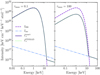 |
Fig. A.1. Intensity of the radiation emerging from a homogeneous, slab-like atmosphere with pure isotropic scattering at an angle of θ = 60°. The slab is illuminated by Iinc ∝ E−1 from the top and by black body radiation from the bottom, IBB(kTe) with kTe = 0.35 keV. The results are presented for two different total optical depths: τmax = 0.1 (left) and τmax = 100 (right). |
A.2. Self-emitting slab with magnetic Compton scattering and absorption
To verify our code for the case of Compton scattering with partial energy and angular redistribution in a magnetized atmosphere, we reproduce calculations of Meszaros & Nagel (1985a). Specifically, we consider a self-emitting homogeneous slab with scattering and free–free absorption and emission. Cross sections of the processes are given by the formulas in Sect. 2.3, but with mixed plasma and vacuum normal modes of photons propagating inside the medium. We solve Eq. (19) in two polarization modes. Following Meszaros & Nagel (1985a), the source function is given by Eq. (20), omitting, however, the additional source of the cyclotron photons, Scyc. The only source of photons in the atmosphere is free–free emission. The upper boundary condition is that there is no illuminating radiation from above

There is no incident radiation from below as well. In this case, due to the symmetry of the problem, only a half of the slab can be considered, with a lower boundary condition set at the middle of the slab

We follow Sect. IVa of Meszaros & Nagel (1985a), assuming that the magnetic field is perpendicular to the surface of the slab with Ecyc = 38 keV. The slab of thickness R = 100 cm has a homogeneous structure with density ρ = 0.5 g cm−3 and a temperature of kTe = 8 keV. We simulate the radiative transfer with four angles chosen, as before, according to the double Gauss-Legendre quadrature (θ = 21°, 48°, 71°, and 86°). We show the resulting angle-integrated flux in Fig. A.2 together with the solution obtained by Meszaros & Nagel (1985a, their Fig. 3a). There are only very small deviations between both solutions, probably due to the different energy grids chosen.
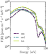 |
Fig. A.2. Flux emerging from a homogeneous self-emitting atmosphere. Grey markers (circles, squared, and triangles) denoting extraordinary, ordinary, and the sum over two polarization modes, respectively, are from Meszaros & Nagel (1985a, Fig. 3a). Colored lines are the result of our simulations with the FINRAD code. |
All Tables
All Figures
|
Fig. 1. Schematic depiction of the model describing the accretion at low Ṁ onto the polar cap of a magnetized neutron star. The polar cap is an emitting layer of an atmosphere with the total column density ymax (corresponding to the total geometrical depth zmax ∼ 10 m) and radius r0. The characteristic stopping length is denoted z0 (geometrical scale) and y0 (column density scale). |
| In the text | |
|
Fig. 2. Total cross section for magnetic Compton scattering (purple lines) and the free–free absorption coefficient (cyan lines) for the ordinary (solid) and extraordinary (dashed) polarization mode, taking into account vacuum polarization. Left: coefficients for a tenuous and hot plasma with ne = 1020 cm−3 and kTe = 35 keV, as expected for the upper, overheated layers of the atmosphere. Right: same but for cold and dense plasma with ne = 1025 cm−3 and kTe = 2 keV, corresponding to the bottom part of the atmosphere. The cyclotron line energy is Ecyc = 75 keV and the incident photon has a direction of θ = 60° with respect to the magnetic field, for both cases. |
| In the text | |
|
Fig. 3. Flowchart of the complete numerical solution. |
| In the text | |
|
Fig. 4. Left: emerging spectrum in two polarization modes. Solid lines describe the total flux, dotted lines extraordinary, and dashed lines ordinary photons. Right: atmospheric structure: electron temperature (solid) and number density (dash-dotted). The major spectral components and associated formation regions are indicated in both panels. |
| In the text | |
|
Fig. 5. Top: photon density at different optical depths of the neutron star atmosphere, τT, summed over polarization modes. The set of model parameters is the same as in Fig. 4. Bottom: photon density integrated over photon energies in each polarization mode. Markers correspond to the lines of a similar color in the top panel; circles indicate ordinary and crosses extraordinary photons. |
| In the text | |
|
Fig. 6. Dependency of the emerging spectra (left column) and atmospheric structure (right column) on the model parameters. The spectra are shown in energy flux times polar cap area, i.e., in luminosity units, for both polarization modes. From top to bottom, we show how the spectral shape and the structure of the atmosphere depend on the mass-accretion rate, Ṁ (a), the polar cap radius, r0 (b), the cyclotron energy, Ecyc (c), and the fraction of the accretion energy going into nonthermal collisional excitations, fcyc. The same baseline model is shown in purple in all panels. See text for further discussion. |
| In the text | |
|
Fig. 7. Unfolded spectrum of the low-luminosity observation of GX 304−1 in EF(E) with the best-fit model (solid black line) for NuSTAR FPMA (blue), FPMB (violet), and Swift/XRT (cyan). For clarity we rebinned the spectra with larger bins for plotting than the ones used for the fit (top). Ratio for the best-fit model (bottom). |
| In the text | |
|
Fig. 8. Parameter probabilities for the polcap model applied to the low-luminosity observation of GX 304−1. Correlations for different parameters are shown in color as two-dimensional confidence maps, where dotted, dashed, and solid contours correspond to the 99%, 90%, and 68% confidence regions, respectively. Here “ΔC-Stat” represents the statistic change compared to the best fit. Side panels on the right show the one-dimensional parameter probabilities. |
| In the text | |
|
Fig. A.1. Intensity of the radiation emerging from a homogeneous, slab-like atmosphere with pure isotropic scattering at an angle of θ = 60°. The slab is illuminated by Iinc ∝ E−1 from the top and by black body radiation from the bottom, IBB(kTe) with kTe = 0.35 keV. The results are presented for two different total optical depths: τmax = 0.1 (left) and τmax = 100 (right). |
| In the text | |
|
Fig. A.2. Flux emerging from a homogeneous self-emitting atmosphere. Grey markers (circles, squared, and triangles) denoting extraordinary, ordinary, and the sum over two polarization modes, respectively, are from Meszaros & Nagel (1985a, Fig. 3a). Colored lines are the result of our simulations with the FINRAD code. |
| In the text | |
Current usage metrics show cumulative count of Article Views (full-text article views including HTML views, PDF and ePub downloads, according to the available data) and Abstracts Views on Vision4Press platform.
Data correspond to usage on the plateform after 2015. The current usage metrics is available 48-96 hours after online publication and is updated daily on week days.
Initial download of the metrics may take a while.