| Issue |
A&A
Volume 650, June 2021
|
|
|---|---|---|
| Article Number | A119 | |
| Number of page(s) | 13 | |
| Section | Interstellar and circumstellar matter | |
| DOI | https://doi.org/10.1051/0004-6361/202040104 | |
| Published online | 16 June 2021 | |
Streaming instability in a global patch simulation of protoplanetary disks
1
Max-Planck-Institut für Astronomie,
Königstuhl 17,
69117
Heidelberg,
Germany
e-mail: This email address is being protected from spambots. You need JavaScript enabled to view it.
2
Dipartimento di Fisica, Universitá di Torino,
via Pietro Giuria 1
(10125)
Torino,
Italy
Received:
10
December
2020
Accepted:
28
March
2021
Abstract
Aims. In recent years, sub-millimeter (mm) observations of protoplanetary disks have revealed an incredible diversity of substructures in the dust emission. An important result was the finding that dust grains of mm size are embedded in very thin dusty disks. This implies that the dust mass fraction in the midplane becomes comparable to that of the gas, increasing the importance of the interaction between the two components there.
Methods. We use numerical 2.5D simulations to study the interaction between gas and dust in fully globally stratified disks. To this end, we employ the recently developed dust grain module of the PLUTO code. Our model focuses on a typical T Tauri disk model, simulating a short patch of the disk at 10 au which includes grains of a constant Stokes number of St = 0.01 and St = 0.1, corresponding to grains with sizes of 0.9 cm and 0.9 mm, respectively, for the given disk model.
Results. By injecting a constant pebble flux at the outer domain, the system reaches a quasi-steady state of turbulence and dust concentrations driven by the streaming instability. For our given setup, and using resolutions up to 2500 cells per scale height, we resolve the streaming instability that leads to local dust clumping and concentrations. Our results show dust density values of around 10–100 times the gas density with a steady-state pebble flux of between 3.5 × 10⁻⁴ and 2.5 × 10⁻³ MEarth yr−1 for the models with St = 0.01 and St = 0.1.
Conclusions. Grain size and pebble flux for model St = 0.01 compare well with dust evolution models of the first million years of disk evolution. For those grains, the scatter opacity dominates the extinction coefficient at mm wavelengths. These types of global dust and gas simulations are a promising tool for studies of the gas and dust evolution at pressure bumps in protoplanetary disks.
Key words: hydrodynamics / accretion, accretion disks / instabilities / turbulence
© M. Flock and A. Mignone 2021
 Open Access article, published by EDP Sciences, under the terms of the Creative Commons Attribution License (https://creativecommons.org/licenses/by/4.0), which permits unrestricted use, distribution, and reproduction in any medium, provided the original work is properly cited.
Open Access funding provided by Max Planck Society.
1 Introduction
The interaction between gas and dust is a crucial part of planet formation. Once grains collide in protoplanetary disks, they are able to stick to one another and grow, which leads to them decoupling from the gas motion (Safronov 1972; Whipple 1972; Adachi et al. 1976; Weidenschilling 1977; Wetherill & Stewart 1993). Once grains settle to the midplane, they concentrate, speeding up the dust coagulation and growth even further (Weidenschilling 1997, 2000; Stepinski & Valageas 1997; Laibe et al. 2008; Brauer et al. 2008; Birnstiel et al. 2011). Depending on the radial profiles of temperature and density, these dense dust layers are prone to other types of instabilities, especially the gas and dust drag instabilities (Squire & Hopkins 2018; Hopkins & Squire 2018; Zhuravlev 2020). The streaming instability (SI), one important branch of these dust drag instabilities, has been studied extensively in the last two decades, in particular for its role in explaining planetesimal formation (Youdin & Goodman 2005; Johansen & Youdin 2007; Bai & Stone 2010; Yang & Johansen 2014; Carrera et al. 2015, 2021; Yang et al. 2017; Schreiber & Klahr 2018). The growth rate of the SI depends on the local dust-gas-mass ratio and can reach values of around the orbital timescale for dust-to-gas mass ratios close to unity (Squire & Hopkins 2018; Pan & Yu 2020). Recent works focused on the SI with multi-grain species (Laibe & Price 2014; Krapp et al. 2019; Zhu & Yang 2021; Paardekooper et al. 2020), demonstrating that its growth rate is in general reduced when considering multiple grain sizes. Lagrangian and fluid methods were used in the past and both have their advantages and disadvantages. As Lagrangian methods introduce a fixed number of grains, in stratified disk models this means that they can only resolve a certain height of the dust disk and one has to ensure good sampling to suppress the noise level (Cadiou et al. 2019). On the other hand, they allow individual grain motions to be followed, and are particularly suited to studying larger grains, which decouple from the gas motion.
Recent studies emphasized again the importance of the level of gas turbulence when determining where the SI can operate (Jaupart & Laibe 2020; Umurhan et al. 2020). So far, most simulations have been performed in local box simulations, and only recently did globally unstratified simulations come into use (Kowalik et al. 2013; Mignone et al. 2019), confirming the main characteristics of the SI. Very recently, Schäfer et al. (2020) investigated the interplay between the vertical shear instability and the SI in stratified global models, demonstrating the importance of the large-scale gas motions for the dust concentrations.
In the present work, we propose a framework to study the SI in globally stratified disk simulations with more realistic conditions for the radial pressure gradient profile and the pebble flux. To the best of our knowledge, this is the first time that the SI is investigated in high-resolution globally stratified simulations using spherical geometry. The challenge is twofold: first, the SI requires resolutions of several hundred cells per gas scale height, and second, the finite extent in the radial direction introduces a time limit to study the SI as the grains radially drift through the domain. In Sect. 2, we explain the numerical method and the disk setup, while in Sect. 3 we present the results and compare them to local box simulation, emphasizing the role of the pebble flux compared to the classical total dust-to-gas mass ratio. Finally, we test our results with constraints from typicalT Tauri star disk systems and dust evolution models and provide estimates of the optical depth at mm wavelengths. We present a discussion and our conclusions in Sects. 4 and 5.
2 Methods and disk setup
In order to setup our model we follow the work of Nakagawa et al. (1986), which prescribes the dust and gas velocities (v and V, respectively) using cylindrical geometry (R, ϕ, Z) as
![Mathematical equation: \begin{align}V_{\textrm{R}} &\,{=}\, {-}\frac{\rho}{\rho+\rho_{\textrm{d}}} \frac{2 D \Omega_{\textrm{K}}}{D^2+\Omega_{\textrm{K}}^2}\eta R \Omega_{\textrm{K}}\\V_{\phi} &\,{=}\, \left(1-\frac{\rho}{\rho+\rho_{\textrm{d}}} \frac{D^2}{D^2+\Omega_{\textrm{K}}^2}\eta \right) R \Omega_{\textrm{K}}\\v_{\textrm{R}} &\,{=}\, \frac{\rho_{\textrm{d}}}{\rho+\rho_{\textrm{d}}} \frac{2 D \Omega_{\textrm{K}}}{D^2+\Omega_{\textrm{K}}^2}\eta R \Omega_{\textrm{K}}\\v_{\phi} &\,{=}\, \left [1+\left (\frac{\rho_{\textrm{d}}}{\rho+\rho_{\textrm{d}}} \frac{D^2}{D^2+\Omega_{\textrm{K}}^2}-1\right)\eta \right] R \Omega_{\textrm{K}},\end{align}](/articles/aa/full_html/2021/06/aa40104-20/aa40104-20-eq1.png)
where ρ and ρd denote, respectively, the gas and dust density,  is the Keplerian frequency with the gravity constant G, and M is the mass of the star. We define the factor
 (5)
(5)
with the dust to gas mass ratio ϵ = ρd∕ρ and the dimensionless Stokes number St = tsΩK with ts being the stopping time. Likewise, we introduce
 (6)
(6)
where P is the (gas) pressure. We note here the factor of 1∕2, which was also adopted by Youdin & Johansen (2007). With this, the pure gas azimuthal velocity translates to vϕ = (1 − η)RΩ1. We assume a local isothermal equation of state with the pressure defined by  with cs (R) being the speed of sound. The scale height H of the gas is defined as H = cs∕ΩK with radial dependence
 (7)
(7)
where P and Q are the radial profile exponents for the density and temperature  .
.
The initial profile of the gas density in the R − Z plane is set by
![Mathematical equation: \begin{equation*}\rho (R,Z)\,{=}\, \rho_0 \left (\frac{R}{R_0} \right)^P \exp\left[\frac{R^2}{H^2}\left(\frac{R}{r} - 1 \right)\right]\,,\end{equation*}](/articles/aa/full_html/2021/06/aa40104-20/aa40104-20-eq8.png) (8)
(8)
where  is the spherical radius.
The dust density ρd is defined similarly to Eq. (8) with the dust scale height Hd:
![Mathematical equation: \begin{equation*}\rho_{\textrm{d}} (R,Z)\,{=}\, \rho_{d,0} \left (\frac{R}{R_0} \right)^P\exp\left[\frac{R^2}{H_{\textrm{d}}^2} \left(\frac{R}{r} - 1\right)\right].\end{equation*}](/articles/aa/full_html/2021/06/aa40104-20/aa40104-20-eq10.png) (9)
(9)
Finally, the initial total dust to gas mass ratio is defined through the ratio of the vertically integrated surface densities, that is, Σd,0 ∕Σ0, related to the midplane densities as
 (10)
(10)
for the gas and for the dust using Σd,0 and Hd,0 respectively. The parameters for the model are summarized in Table 1.
Initial setup parameters for the 2D dust and gas disk models.
2.1 Numerical configuration
We performed our computations in spherical geometry using the Harten, Lax, and van Leer (HLL) Riemann solver and the second-order Runge–Kutta integration in time to advanced conserved variables. Also, we used the piece-wise linear reconstruction with the monotonized central (MC) limiter. We handle the gravity force by adding the vector force on the right-hand side of the momentum equation for both gas and particles. The radial boundary conditions for the hydro variables are zero-gradient without allowing for material to enter the domain. This is obtained by setting the normal velocity component to zero in case the velocity in the active domain is pointing inward. At the meridional boundary, ghost zones are filled by extrapolating the exponential profile of the gas density while the remaining variables are set to have zero gradient. Similarly to the radial boundaries, gas is not allowed to enter the domain. Dust particles are advanced in time using the exponential midpoint method andwe use the cloud-in-cell (CIC) weighting scheme to determine the gas values at the grain position (Mignone et al. 2019). We use mutual feedback terms to couple gas and dust, and account for drag force effects. As particles arestored locally on each processor, we reach best parallel performance when we use a decomposition X: 2 for the r: θ domain. Formore information about the method we refer to our previous work (Mignone et al. 2019).
We note that the resolution was chosen to resolve the grain drag and therefore the grid size should fulfill
 (11)
(11)
in order to resolve the grain stopping length; for our setup with a fixed Stokes number, this becomes Δx < StH. Further, we have to resolve the SI for the regimes of St = 0.1 and St = 0.01 and we adopt a grid resolution similar to that used by Yang et al. (2017) with around 1000 cells per H. The aspect of resolution is discussed in detail in Sect. 4.2. We use a uniform grid spacing in the radial and in the θ direction. The total number of grid cells and domain extent are given in Table 2.
Overview of numerical models.
2.2 Lagrangian particle setup
In order to sample the dust density we introduce individual particles to the simulation. Those particles represent a swarm of grains. Similar to the work by Yang et al. (2017), we start the simulation assuming a dust scale height which is reduced compared to the gas scale height. This locally increases the dust-to-gas-mass ratio and enhances the growth rate of the SI.
We present our results using particle sample runs with approximately 80 particles per cell for model ST1 and 5 particles per cell for model ST2. For our models, we determined that a sampling of around five cells or more is needed for consistent results. More details on the sampling and a benchmark can be found in Appendices A and B.
The total dust mass in the domain is
 (12)
(12)
Using a total number of grains of Ntot = 1.04 × 10⁷, we sample the dust mass in our domain with particle swarms with masses of 1.902 × 10⁻⁷ Earth masses.
Once the mass of the particle is fixed, the number of particles in each cell can be determined with Ncell = (ρdΔV)∕mg. A vertical profile of the detailed sampling over height is shown in Appendix A.
The initial profile of the gas and dust density in the R–Z plane is shown in Fig. 1. As seen in the contour plot, the particle method can only resolve a certain vertical extent which depends on the total number of grains. The initial gas and dust velocities are plotted in the bottom panel of Fig. 1, following the equilibrium solutions in Eqs. (1)–(4).
In this equilibrium solution, at the midplane, the grains slowly drift radially inward while the gas slowly drifts radially outward.
2.3 Damping zones
To prevent numerical effects from the radial domain boundary, we need to implement a buffer zone in which the variables of density and velocity are relaxed back to their initial values. To this end, we apply wave-killing zones close to the radial inner and outer boundary to reduce the interaction with the boundary. Similar buffer zones were already tested and implemented in our previous work Mignone et al. (2019). In these zones, the variables are relaxed to the initial equilibrium values,
![Mathematical equation: \begin{equation*}Q({\vec{x}},t)\,{=}\,Q_0({\vec{x}})+ \Big[Q({\vec{x}},t) - Q_0({\vec{x}})\Big]e^{F(R) \Delta t/T}\,,\end{equation*}](/articles/aa/full_html/2021/06/aa40104-20/aa40104-20-eq14.png) (13)
(13)
where Q(x, t) represents either the radial or azimuthalfluid velocity, Q0(x) is the corresponding equilibrium value, T = 1.0 and
 (14)
(14)
is a tapering function with w = 0.05.
A second important point is to prevent the dust dragging the gas material out. As we constantly inject new grains at the radial outer zone we also have to replenish the gas material. To study the SI in a quasi-steady state configuration, we implement a density relaxation that relaxes the loss of gas mass to the initial value. For each grid cell, we apply
![Mathematical equation: \begin{equation*}\rho(r,\theta)\,{=}\,\rho_0(r,\theta)+ \Big[\rho((r,\theta),t) - \rho_0(r,\theta)\Big]e^{2 \Delta t/T}\,,\end{equation*}](/articles/aa/full_html/2021/06/aa40104-20/aa40104-20-eq16.png) (15)
(15)
setting the parameter T = 1.0. In Appendix C, we show that the influence of parameter T in this regime of the density relaxation remains small.
2.4 Injection and destruction of particles
At the outerboundary, new particles must be constantly injected as the radial drift empties these buffer zones. Refilling has to be done carefully as in this model the vertical settling quickly changes the structure in the buffer zones. To prevent the solution from quickly shifting away from the equilibrium solution, we damp the vertical velocity as long as the particles remain in the outer buffer zone. More specifically, at every time-step we set
 (16)
(16)
in the radial outer buffer zone using χ = 10−5. We find that this efficiently prevents the particles from settling to the midplane before they have entered the active domain. In addition, we inject only dust when the dust density drops below a certain factor f, which is ρd <fρd,0 with f = 0.5 for St = 0.1 particles and f = 0.25 for St = 0.01. In this way, we are able to resupply the disk with a constant pebble flux without any accumulation at the buffer zone edges. Particles are constantly injected in r ∈ [10.6, 10.7] au as they radially drift inward. For r < 10.6 au, they start to settle, eventually triggering the SI. At around 10.5 au and inwards, the structure and the dynamics of the dust and gas remain self-similar.
Particles are removed from the computational domain once they cross the inner boundary at 9.3 au. To avoid dust accumulation at the inner buffer zone we reduce the azimuthal velocity through
 (17)
(17)
at every time-step in the inner buffer zone using χ = 10−8. This reduces their rotational velocity, thus increasing their radial drift to avoid any concentration close to the buffer zone edge at 9.4 au.
2.5 Particle size
In our models, we fix the Stokes number of the grains which makes comparison to previous works easier. As the gas density in our domain does not vary significantly, we can determine the approximate size of the dust grains. For our disk setup, we are in the Epstein regime and we can determine the size using
 (18)
(18)
where, for the grain density, we employ ρgrain = 2.7 g cm−3. Using the midplane density at 10 au we determine the grain sizes of 0.88 mm for model ST2 and 8.8 mm for model ST1.
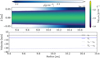 |
Fig. 1 Top: initial distribution of the gas and dust density in the R-Z plane. Bottom: initial radial profile of the gas and dust velocities at the midplane. |
3 Results
After a few orbits, the dust settles to the midplane and radially drifts further inwards. At the same time, the SI is triggered leading to concentration and clumping of the dust. Dust grains are resupplied to the outer buffer zones, enabling a constant pebble flux. In the following, we investigate the dust concentrations and scale height in our models.
3.1 Dust concentration and streaming instability
In the following, we analyze the maximum dust density at the center of the domain at 10 au in a small radial patch of 0.1 au. Our results, plotted in Fig. 2, show that after roughly ten orbits the dust concentration reaches up to 100 times the initial value. Grains with St = 0.1 (top panel in Fig. 2) show a strong concentration, attaining a (temporally averaged) maximal dust-to-gas-mass ratio of ϵmax = 24 ± 14. The average concentration level at the midplane saturates at the time-averaged value of ϵ = 4 with a large scatter. Grains with St = 0.01 (bottom panel in Fig. 2) show slightly lower concentrations with (temporally averaged) maximum concentrations of around 10 ± 3 of the dust-to-gas-mass ratio. The spatially averaged midplane value of the dust-to-gas-mass ratio is 2.8.
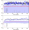 |
Fig. 2 Maximum dust-to-gas-mass ratio at 9.5 au (blue) and at 10 au (black) for model ST1 (top) and model ST2 (bottom). The space-averaged dust-to-gas-mass ratio at the midplane is shown with the red solid line, including the standard deviation (filled color). |
3.2 Surface density evolution
Figure 3 shows the evolution of the vertically integrated dust surface density for both models. After 10 orbits, the SI transforms the smooth surface density into dust fragments of low and high dense filaments. The top panel of Fig. 3 shows narrow, close-to-horizontal stripes, which indicate the fast inward radial drift for model ST1. At ~ 80 and ~ 100 orbits, two large dust accumulations become visible in the surface density, which leads to a reduction of the radial drift. This is to be expected because large dust clumps can shield each other from the gas headwind. In these large dust clumps, the maximum dust concentration can lead to dust-to-gas-mass ratios of approximately 100; see the top panel of Fig. 2, close to 90 orbits.
The bottom panel of Fig. 3 displays the temporal evolution of the dust surface density for model ST2. Here, the SI also leads to overdense structures in the surface density. Due to the slower inward radial drift, the dust clumps show a broader structure over time. The concentrations in the surface density remain at a similar level as those of model ST1 although we do not observe the large dust accumulations.
Figure 4 shows snapshots of the dust density after ~ 100 orbits for both models in the meridional plane. The dust layer is very thin, with a vertical extent of only 0.01 au and attaining dust densities of around 10−11 g cm−3. Figure 4 (top panel) shows dust clumps for model ST1 on top of the narrow dust layer that remains concentrated in a region corresponding to roughly 1% of the gas scale height. The turbulent structures have sizes of around one-tenth of the gas scale height in radius, while there is a sharp density contrast along the vertical direction. Likewise, we show the snapshot for model ST2 (bottom panel of Fig. 4). Here, the turbulent structures appear much finer compared to those of model ST1, and have a smoother density contrast in the vertical direction.
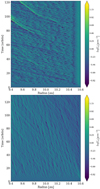 |
Fig. 3 Temporal evolution of the dust surface density over time for model ST1 (top) and model ST2 (bottom). |
3.3 Vertical dust scale height and effective α
To calculate the dust scale height, we follow first the approach by Yang et al. (2017) and determine the standard deviation of the vertical position of the grains as
 (19)
(19)
where z = Rcos θ. Figure 5 shows the evolution of the dust scale height over time which remains between 0.2% and 0.3% of the gas scale height for both models.
To verify the scale height determined using this latter technique, we follow another approach outlined in Flock et al. (2020) and plot the averaged vertical dust density profile (see Fig. 6). The plot provides the time-averaged profile from 20 orbits until the end of the simulation and spatially averaged at 10 au ± 0.15 au. The dust density is normalized by the gas density (which remains effectively flat in the vertical direction with only deviations of the order 10−3). Both profiles fit best with a value for Hp∕H of ~ 0.003, particularly inside the first 0.01 au from the midplane. Above 0.01 au from the midplane, the profile becomes shallower, probably because of sudden bursts of dust clumps, as seen in Fig. 1. By determining the dust scale height, we can effectively determine the level of equivalent turbulence required to produce such a profile.
Following the calculation from our previous work Flock et al. (2020) and Dubrulle et al. (1995), we estimate the turbulent diffusivity α with
 (20)
(20)
assuming a Schmidt number Sc of unity. Inserting the values for the Stokes numbers we derive an effective α of about 10−6 for model ST1 and 10−7 for model ST2.
4 Discussion
4.1 Comparison to previous local box simulations
In what follows, we compare our simulation results with previous stratified local box models of the SI. Two parameters are important for the characterization of the evolution of the SI, namely, the Stokes number and the value of σd = Σd∕(ρ0ηr) which can be understood as an average dust-to-gas-mass ratio at the midplane layer. Most of the dust mass is concentrated in a region of 1% of the gas scale height around the midplane, which motivates the need to quantify the SI using different parameters, as demonstrated by Sekiya & Onishi (2018) who adopted σd. These latter authors introduced the parameter σd based on 3D stratified local box simulations.
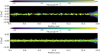 |
Fig. 4 Distribution of the dust density after 100 orbits for model ST1 (top) and model ST2 (bottom). |
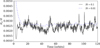 |
Fig. 5 Evolution of dust scale height over time, shown for models ST1 and ST2. |
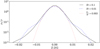 |
Fig. 6 Vertical profile of the dust-to-gas-mass ratio, time and space averaged at 10 au, for models ST1 and ST2. A fitting profile is shown with the red dotted line. |
Maximum dust-to-gas-mass ratio
Our models have St = 0.1 (ST1) and St = 0.01 (ST2) with σd = 0.36. Sekiya & Onishi (2018) presented a variety of simulation cases, the closest of which are their models (A) with (St = 0.1, σd = 0.5) and model (G) with {St = 0.01, σd = 0.5}. While our model ST1 favorably compares (in terms of the maximum dust concentration) to their model (A) (ϵmax ~ 24 versus ϵmax ~ 10), we found higher values for ϵmax for our model ST2 compared to their model (G) (ϵmax = 10 versus ϵmax = 2.4).
Dust scale height
In Sect. 3.3, we show that the dust scale height in steady state reaches values of Hp ∕H = 0.003. Because of the different convention in local box simulations our H is a factor of  larger and
  . To be able to compare with the previous local box simulations we include this factor, which gives Hp ∕Hl = 0.0042.
Yang et al. (2017) found a dust vertical scale height for St = 0.01 grains and σd = 1 of about Hp = 0.014, which is roughly three times higher than in our models. Carrera et al. (2015) presented a model with σd = 0.5 and his particle scale height was around Hp = 0.005, very similar to the value we find. Sekiya & Onishi (2018) found that the strength of the SI scales with σd, a result also predicted from the analytical works of Squire & Hopkins (2018); Pan & Yu (2020) who demonstrated that the growth rate depends on the dust-to-gas-mass ratio. As our models adopt a lower value of σd, it might be that the strength of the SI is reduced.
Dust clumping
Yang et al. (2017) found long-lasting dust concentrations appearing after hundreds to thousands of orbits, while Sekiya & Onishi (2018) noticed that such concentrations appear for values of σd ≥ 1. Model ST1 showed two events of secondary dust concentration reaching values of 100 times the gas density, which reduced the radial drift of the dust clump, although this concentration was not enough to reach the critical Roche density; see Appendix D. On the other hand, model ST2 showed no major dust concentration. We also note that such dust accumulations have been observed on timescales of several hundreds of orbits (Yang et al. 2017). The radial drift in combination with our limited radial domain extent does not allow us to trace individual grains for such a long time (we cannot follow individual grains for more than around ten orbits in model ST1).
We therefore conclude that our simulation results show similar values of dust clumping as observed in local box simulations. We find a smaller value of the dust scale height and no secondary long-lasting dust accumulation, both possibly because of our choice of σd.
Finally, we performed a local box simulation with the same setup as presented in Yang et al. (2017) in Appendix E in order to compare our new numerical method to previous models. We report that the results of dust concentration and particle vertical mixing in our local box runs are very similar to those found in previous works.
4.2 Resolving the streaming and other instabilities
Both grid resolution and particle sampling are important to correctly represent and resolve the dust and gas interactions.
Grid resolution is crucial to resolving the fastest growing modes of the SI. Squire & Hopkins (2018) pointed out that the wavenumber of the fastest growing mode for the SI follows roughly kηr ~ 1∕St. In our model ST1, assuming k ~ 1∕Δx and 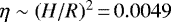 we obtain H2 ∕(RΔr) ~ 45, which allows us to resolve wavenumbers (ideally) up to 45 using 640 zones per scale height. Here, the fasting growing mode corresponding to kηr ~ 10 is well resolved. Model ST2 can capture wavenumbers kηr up to 180 and so also resolves the fastest growing mode corresponding to kηr ~ 100. Yang et al. (2017) showed SI operating with St = 0.01 with a range of resolutions from kηr = 32 up to 256 while the strongest concentrations appeared when using resolutions close to the fastest growing wavelength.
Accurate particle sampling is fundamental to correctly capturing the dust feedback and to resolving the dust distribution (Mignone et al. 2019). Sekiya & Onishi (2018) adopt a particles-to-grid-cells ratio of Npar∕Ncell ≈ 1.39 while Yang et al. (2017) used a ratio of unity. In our models we employ Npar∕Ncell ≈ 79.3 for model ST1 and Npar∕Ncell ≈ 4.95 for model ST2, both much larger than the previous models. In the Appendix of Yang et al. (2017), this author compares results obtained using Npar∕Ncell = 10 and Npar∕Ncell = 1 and finds no significant difference. From this perspective, our models provide the necessary grid resolution and particle sampling to capture the basic SI properties and to resolve for the dust feedback.
Another type of instability which might have an important effect is the vertical shear SI (Ishitsu et al. 2009) which is driven by the vertical gradient of the velocity shear between the dust and the gas. A recent work by Lin (2021) emphasizes the role of this instability in determining the vertical scale height of the dust. However, we point out that scales of the order of 10−3H have to be resolved to capture the vertical shear SI. Future high-resolution simulations reaching ten thousand cells per H are needed to verify the importance of new types of instabilities, like the settling instability or the vertical shear streaming instability.
4.3 Gas transport
Without damping, the gas surface density is quickly reduced, creating strong radial pressure gradients which affect the gas surface density structure. Owing to the limited domain extent, we were not able to investigate this interesting effect. As a result of the small vertical domain in particular, this effect is enhanced as there is no resupply of gas material from the upper layers. For these, models we applied the gas density relaxation to study the SI in quasi-steady state in more detail. Future simulations should include a much larger vertical extent to examine the effect of the dust drag on the gas, particularly in regions where dust is expected to accumulate, such as the water ice line where the dust drag can become very important for the gas motion (Gárate et al. 2020).
4.4 Regions of planetesimal formation
Over recent years, several works have shown that the generation of planetesimals via the SI in a smooth disk profile remains difficult. First, a large amount of solid material (Z > 0.02) – larger than the typical ISM value – has to be provided in a single dust species of a particular Stokes number (Yang et al. 2017; Johansen et al. 2014), leaving a relatively narrow range of parameters (Umurhan et al. 2020; Chen & Lin 2020), even more narrow when including the effect of turbulence (Jaupart & Laibe 2020). However such favorable conditions – a low amount of turbulence and a narrow range in mass distribution of large grains – is not expected from dust evolution models (Brauer et al. 2008; Birnstiel et al. 2011). Another difficulty arises in multi-grain simulations including different grain sizes, which showed the reduction of the SI growth regime (Krapp et al. 2019).
On the other hand, the locations of pressure maxima in the disk remain plausible regions for planetesimal formation, owing to the large dust concentration and the favorable conditions in which the SI can operate (Auffinger & Laibe 2018; Abod et al. 2019; Carrera et al. 2021).
4.5 The importance of the pebble flux
With the present work we intend to emphasize the importance of the radial flux of pebbles rather than adopting the (more common) total gas-to-dust-mass ratio when modeling the evolution of the SI. The pebble flux controls the transport of the solid material in the disk, it can show us where dust grains get concentrated and trapped, and it is important for the accretion of solid material onto planets (Ormel & Liu 2018) which requires an understanding of their vertical distribution (Laibe et al. 2020). The radial flux of pebbles can be determined using dust growth and evolution models (Birnstiel et al. 2012; Takeuchi & Lin 2002; Drążkowska et al. 2016; Drazkowska et al. 2021).
Using the pebble flux simulator2 we determine the pebble flux over time using the same disk profile employed in our simulations. The method and further references of the tool can be found in Drazkowska et al. (2021). The results are shown in Fig. 7. The maximum pebble flux is reached at around 104 yr and matches the value obtained in our model ST2, approximately Ṁd ~ 3.5 × 10⁻⁴MEarth yr−1 (see Fig. 7 top). The pebble flux and grain sizes in model ST1 lie above the predicted values from the dust evolution models.
We then conclude that our model ST2 using (St = 0.01, σd = 0.36) presents realistic conditions in terms of the amount of dust when compared to models of dust evolution. However, such initial conditions are not favorable for secondary dust clumping events by the SI (Sekiya & Onishi 2018), which are needed to account for planetesimal formation (Yang et al. 2017). This is an important aspect which should be investigated in more detail in forthcoming simulations of the SI.
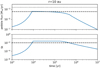 |
Fig. 7 Pebble flux over time, calculated with the pebble predictor tool using the same disk initial conditions. Overplotted are the values from our simulation results, from model ST1 (dotted line) and model ST2 (dashed line). |
4.6 Total optical depth at mm wavelengths
An important question remains as to whether the dust layer observed in protoplanetary disks is optical thin or thick at a given wavelength. For this, we calculate the opacity of the two grain sizes at the wavelength of λ = 1.3 mm corresponding to the ALMA Band 6 observations. To calculate the opacity, we use the optool3 which uses the DIANA dust properties (Toon & Ackerman 1981; Woitke et al. 2016) and includes the distribution of hollow spheres method (Min et al. 2005) to calculate the dust opacity. For the specific settings we use amorphous pyroxene (70% Mg) with a mass fraction of 87% and 13% of amorphous carbon (Zubko et al. 1996; Preibisch et al. 1993) and a water ice mantel with a mass fraction of 20% and a porosity of 20%. We calculate the opacity for the two grain sizes using narrow size bins of (0.8–1 mm) and (0.8–1 cm) for model ST2 and model ST1, respectively. The corresponding absorption and scatter opacity at λ = 1.3 mm for model ST2 are κabs = 3.009 cm2 g−1, κscat = 21.957 cm2 g−1 and for model ST1 these are κabs = 0.635 cm2 g−1 and κscat = 1.166 cm2 g−1. In Fig. 8, we plot the radial profile of the total optical depth τ = Σdκ calculated for both models using the vertical integrated dust density.
The profiles show that for model ST1, the total optical depth remains around unity, while the optical depth from pure absorption opacity remains mostly optically thin. For model ST2, the grain size is closer to the corresponding wavelength. Here, the optical depth is larger andremains mostly above unity. The scatter opacity is much larger for these grains which leads to a total optical depth of around 10. More and more observations of protoplanetary disks at mm wavelengths confirm the important effect of scattering (Sierra & Lizano 2020). Also, grain sizes of around mm sizes are consistent with the observations (Carrasco-González et al. 2019).
Overall, the variations in τabs caused by the SI fluctuate between 0.4 and 4 (thus a factor of ~ 10) in model ST2 and between 0.02 and 2 (a factor ~ 100) for model ST1. We point out again that these structures are on spatial scales of tens of H, which translates to scales of 0.1 au at a distance of 10 au from the star. Current radio interferometer capabilities of ALMA reach a spatial resolution of 5 au for the dust emission at mm wavelengths in the most nearby star disk systems.
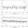 |
Fig. 8 Optical depth τ = Σκ over radius shown for models ST1 (top) and ST2 (bottom). |
5 Conclusions
In this work, we present a new generation of models to investigate the dust and gas drag instabilities in globally stratified simulations of protoplanetary disks. We performed high-resolution, 2D global hydrodynamical simulations, including the dust back-reaction on the gas, modeling the conditions of a protoplanetary disk around a star of one solar mass. Our numerical method is based on the hybrid fluid-particle framework recently developed by Mignone et al. (2019), where the dust component is modeled by Lagrangian particles. We adopt 2D spherical geometry covering the meridional domain (r: θ) with a grid resolution up to 1280 cells per gas scale height to resolve for the streaming instability. The dust grains are modeled with a constant Stokes number of St = 0.1 and St = 0.01 which corresponds to grain sizes of 880 μm and 8.8 mm, respectively,at 10 au. The dust grains radially drift through the domain and undergo streaming instability, leading to the formation of large dust concentrations. By resupplying dust grains to the outer radial domain, we reach a quasi-steady state of pebble flux and operating streaming instability. Our main results may be summarized as follows:
The streaming instability leads to dust clumping, with maximum values of between 10 and 100 in terms of dust-to-gas-mass ratio. The average dust-to-gas-mass ratio at the midplane remains between 2 and 4;
For St = 0.1 we observe the appearance of large dust clumping reaching dust-to-gas-mass ratios above 100 which can effectively reduce the radial drift as grains shield one another from the gas drag;
We find that the dust layer remains concentrated within a region of ±0.01 au around the midplane. Our models show an effective dust scale height of about Hp∕H = 0.003 independent of the Stokes number;
We reach a nominal flux of pebbles of Ṁd ~ 3.5 × 10⁻⁴ MEarth yr−1 (~2.5 × 10⁻³ MEarth yr−1) for grains with St = 0.01 (St = 0.1). The grain size and pebble flux for model St = 0.01 compares best with dust evolution models of the first million years of disk evolution.
We finally wish to emphasize the important role of the pebble flux when determining the amount of dust in simulations of the streaming instability. The maximum pebble flux in the disk is reached during the first million years of disk evolution. T Tauri star disk models with a pebbles flux of around 3.5 × 10⁻⁴ Earth masses per year and Stokes numbers 0.01 ≲St ≲ 0.1 are closed to what is expected from dust evolution models. For this range of parameters, σd remains below unity, making secondary dust clumping for planetesimal formation difficult (Sekiya & Onishi 2018). This novel class of global dust and gas simulations constitutes a promising tool for forthcoming studies targeting gas and dust evolution in protoplanetary disks, especially for situations where the density and pressure are strongly changing (such as at pressure maxima).
Acknowledgements
We thank Jonathan Squire for helpful comments on the manuscript. M.F. acknowledges funding from the European Research Council (ERC) under the European Union’s Horizon 2020 research and innovation program (grant agreement no. 757957). Figures where produced by python matplotlib library (Hunter 2007).
Appendix A Dust sampling
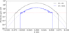 |
Fig. A.1 Number of particles per cell along the vertical direction for both models. The red dotted line marks the position of one particle per cell. |
In our models, the dust density is sampled by individual particles. In Fig. A.1, we show the number of particles per cell along the vertical direction for both models ST1 and ST2 at 10au. The black and blue dotted lines shows the initial dust density profile and the theoretical sampling. The dust density can only be sampled until a given height, where one has at least one particle per cell, as indicated with the red dotted line in Fig. A.1.
Appendix B Benchmark - Dust sampling
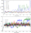 |
Fig. B.1 Benchmark results of model ST1 for different sampling rates, showing the dust scale height (top) and the maximum dust concentration at 10 au. |
Here, we investigate the effect of the particle sampling. For this we perform a series of runs based on model ST1 using different numbers of particles ranging from 0.5 up to 160 particles per cell. Figure B.1 shows the dust scale height and the maximum dust concentration ϵmax at 10 au over time. The results indicate that a sampling of five particles per cell or more is enough to show converging results. Below this value sudden dust concentrations occur which also trigger larger dust scale heights, possibly due to Kelvin–Helmholtz Type instabilities.
Appendix C Gas damping
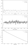 |
Fig. C.1 Comparison results using two runs with different gas relaxation parameter for model ST1. Shown is the dust scale height (top), the maximum dust concentration (middle) and the midplane radial profile of the gas density (bottom). |
As we relax the gas density in our domain we have to verify that the gas damping does not strongly affect the non-linear evolution of the streaming instability. To this end, we performed a test run setting the damping factor T = 10.0 in Eq. (13) for the gas damping, leading to a reduced gas damping rate. The results are summarized in Fig. C.1. The lower gas damping does not strongly effect the main results.
Appendix D Roche density
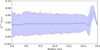 |
Fig. D.1 Maximum dust density over radius, time averaged for model ST1 and normalized over the Roche density. Solid line and filled area present the mean and standard deviation. |
A common approach to investigating whether the SI could produce planetesimals directly through dust clumping which then collapse dueto self-gravity is by determining the Roche density:
 (D.1)
(D.1)
In Fig. D.1, we determine the maximum density (normalized to the Roche density) by computing the value at each radial position and then taking the average value over time. Figure D.1 shows that on average the maximum density concentration at the midplane reaches around ~ 3% of the Roche density. The profile remains very flat with a small rise close to 10.6 au due to the injection of grains in the outer buffer zone. We note that for our models we never reached the Roche density in dust in a single cell.
Appendix E Shearingbox
In order to better compare our results to previous models of the streaming instability using local box simulations we used a model similar to that of Yang et al. (2017). In this model, we solve the axisymmetric shearingbox equations in the (x, z) plane with x, z ∈ [−0.2H, 0.2H] where H = cs∕Ω is the vertical scale height. The module has been thoroughly described in Mignone et al. (2019).
At t = 0, we initialize the fluid state using the Nakagawa equilibrium (Nakagawa et al. 1986):
![Mathematical equation: \begin{equation*}\vec{v}\,{=}\,\displaystyle \frac{\eta v_K}{\Delta}\left[2\epsilon\tilde{\tau}_{\textrm{s}},\,-\frac{\Delta + \epsilon\tilde{\tau}_{\textrm{s}}^2}{1+\epsilon},\,0\right]\,,\end{equation*}](/articles/aa/full_html/2021/06/aa40104-20/aa40104-20-eq26.png) (E.1)
(E.1)
where  ,
,  Here ϵ = 0.01 = ρf∕ρ0 and τs = 0.01 are the dustto gas mass ratio and dust particles stopping time, respectively. Gas density is initially set to unity (ρ0 = 1) and an isothermal equation of state
  is adopted, where cs is the sound speed. Our units are chosen so that Ω = 1 and H = 1 (it naturally follows that cs = 1). The quantity ηvK = 0.05cs represents the external radial pressure gradient included on the gas. As in Yang et al. (2017), we neglect vertical gravity on the gas because no appreciable density stratification is present in the computational domain. We do nevertheless include linearized gravity (gz = − Ω2z) on the particles.
Dust grain velocities are also initialized with the Nakagawa equilibrium,
![Mathematical equation: \begin{equation*}\vec{v}_{\textrm{p}}\,{=}\,{-}\frac{\eta v_K}{\Delta}\left[2\tilde{\tau}_{\textrm{s}},\,\frac{\Delta - \tilde{\tau}_{\textrm{s}}^2}{1+\epsilon},\, 0 \right],\end{equation*}](/articles/aa/full_html/2021/06/aa40104-20/aa40104-20-eq30.png) (E.2)
(E.2)
(we note that an incorrect factor ϵ appears in the expression for vp in Eq. (55) of Mignone et al. 2019) while their position is assigned as
![Mathematical equation: \begin{equation*}\vec{x}_{\textrm{p}}\,{=}\,\left[x_{\textrm{b}} + (i+0.5)\Delta x,\, 0,\, z_{\textrm{p}}\,{=}\,r_{\textrm{g}}\right],\end{equation*}](/articles/aa/full_html/2021/06/aa40104-20/aa40104-20-eq31.png) (E.3)
(E.3)
where xb = −0.2H is the leftmost boundary, i = 0, Nx − 1, Δx is the mesh spacing along the x-direction, and rg is a Gaussian random number with mean μ = 0 and σ = 0.02H. This mimics a spatial distribution of dust of ρf ~ exp(−z2∕2σ2) with reduced scale height in order to shorten the sedimentation phase process as was done in Yang et al. (2017).
Particle mass is prescribed (Eq. (1) of Yang et al. 2017) according to:
 (E.4)
(E.4)
where  is the average number of particles per cell and Nz is the number of cells in the vertical (z) direction. We note that Δy = 1 for our 2D simulations.
We perform computations using the piece-wise parabolic method (PPM) algorithm with the Roe Riemann solver and the FARGO orbital advection scheme (Mignone et al. 2012) through which the boundary conditions in the radial (x) direction become simply periodic. We employ 5762 grid zones in total (equivalent to 1440 zones per scale height) and evolve the system up to 1000 P, where P = 2π∕Ω is the local orbital period.
Results showing the dust density distributions at different times are shown in Fig. E.1. The streaming instability leads to dust clumping and concentrations. After 300 orbits we observe the start of larger clumps, which is often called the secondary phase of dust concentration and was also reported in Yang et al. (2017).
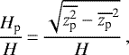
In the top panel of Fig. E.2, we plot the particle scale height Hp ∕H as a function of time with
 (E.5)
(E.5)
The bottom panel of the same figure shows the maximum dust density as a function of time. Both results of the particles scale height and the dust concentration compare very well with the previous findings of Yang et al. (2017).
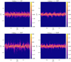 |
Fig. E.1 Dust density colored maps at t∕P = 20, 100 (top panels) and t∕P = 300, 1000 (bottom panels) for the shearingbox model. |
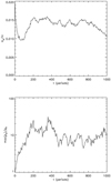 |
Fig. E.2 Particle scale height as a function of time. |
References
- Abod, C. P., Simon, J. B., Li, R., et al. 2019, ApJ, 883, 192 [Google Scholar]
- Adachi, I., Hayashi, C., & Nakazawa, K. 1976, Progr. Theor. Phys., 56, 1756 [Google Scholar]
- Auffinger, J., & Laibe, G. 2018, MNRAS, 473, 796 [Google Scholar]
- Bai, X.-N., & Stone, J. M. 2010, ApJ, 722, 1437 [Google Scholar]
- Birnstiel, T., Ormel, C. W., & Dullemond, C. P. 2011, A&A, 525, A11 [NASA ADS] [CrossRef] [EDP Sciences] [Google Scholar]
- Birnstiel, T., Klahr, H., & Ercolano, B. 2012, A&A, 539, A148 [NASA ADS] [CrossRef] [EDP Sciences] [Google Scholar]
- Brauer, F., Dullemond, C. P., & Henning, T. 2008, A&A, 480, 859 [NASA ADS] [CrossRef] [EDP Sciences] [Google Scholar]
- Cadiou, C., Dubois, Y., & Pichon, C. 2019, A&A, 621, A96 [NASA ADS] [CrossRef] [EDP Sciences] [Google Scholar]
- Carrasco-González, C., Sierra, A., Flock, M., et al. 2019, ApJ, 883, 71 [Google Scholar]
- Carrera, D., Johansen, A., & Davies, M. B. 2015, A&A, 579, A43 [NASA ADS] [CrossRef] [EDP Sciences] [Google Scholar]
- Carrera, D., Simon, J. B., Li, R., Kretke, K. A., & Klahr, H. 2021, AJ, 161, 96 [Google Scholar]
- Chen, K., & Lin, M.-K. 2020, ApJ, 891, 132 [NASA ADS] [CrossRef] [Google Scholar]
- Drążkowska, J., Alibert, Y., & Moore, B. 2016, A&A, 594, A105 [NASA ADS] [CrossRef] [EDP Sciences] [Google Scholar]
- Drazkowska, J., Stammler, S. M., & Birnstiel, T. 2021, A&A, 647, A15 [EDP Sciences] [Google Scholar]
- Dubrulle, B., Morfill, G., & Sterzik, M. 1995, Icarus, 114, 237 [NASA ADS] [CrossRef] [Google Scholar]
- Flock, M., Turner, N. J., Nelson, R. P., et al. 2020, ApJ, 897, 155 [CrossRef] [Google Scholar]
- Gárate, M., Birnstiel, T., Drążkowska, J., & Stammler, S. M. 2020, A&A, 635, A149 [NASA ADS] [CrossRef] [EDP Sciences] [Google Scholar]
- Hopkins, P. F., & Squire, J. 2018, MNRAS, 480, 2813 [NASA ADS] [CrossRef] [Google Scholar]
- Hunter, J. D. 2007, Comput. Sci. Eng., 9, 90 [NASA ADS] [CrossRef] [Google Scholar]
- Ishitsu, N., Inutsuka, S.-i., & Sekiya, M. 2009, ArXiv e-prints [arXiv:0905.4404] [Google Scholar]
- Jaupart, E., & Laibe, G. 2020, MNRAS, 492, 4591 [CrossRef] [Google Scholar]
- Johansen, A., & Youdin, A. 2007, ApJ, 662, 627 [Google Scholar]
- Johansen, A., Blum, J., Tanaka, H., et al. 2014, in Protostars and Planets VI, eds. H. Beuther, R. S. Klessen, C. P. Dullemond, & T. Henning, 547 [Google Scholar]
- Kowalik, K., Hanasz, M., Wóltański, D., & Gawryszczak, A. 2013, MNRAS, 434, 1460 [NASA ADS] [CrossRef] [Google Scholar]
- Krapp, L., Benítez-Llambay, P., Gressel, O., & Pessah, M. E. 2019, ApJ, 878, L30 [NASA ADS] [CrossRef] [Google Scholar]
- Laibe, G., & Price, D. J. 2014, MNRAS, 444, 1940 [NASA ADS] [CrossRef] [Google Scholar]
- Laibe, G., Gonzalez, J. F., Fouchet, L., & Maddison, S. T. 2008, A&A, 487, 265 [NASA ADS] [CrossRef] [EDP Sciences] [Google Scholar]
- Laibe, G., Bréhier, C.-E., & Lombart, M. 2020, MNRAS, 494, 5134 [Google Scholar]
- Lin, M.-K. 2021, ApJ, 907, 64 [Google Scholar]
- Mignone, A., Flock, M., Stute, M., Kolb, S. M., & Muscianisi, G. 2012, A&A, 545, A152 [NASA ADS] [CrossRef] [EDP Sciences] [Google Scholar]
- Mignone, A., Flock, M., & Vaidya, B. 2019, ApJS, 244, 38 [NASA ADS] [CrossRef] [Google Scholar]
- Min, M., Hovenier, J. W., & de Koter, A. 2005, A&A, 432, 909 [NASA ADS] [CrossRef] [EDP Sciences] [Google Scholar]
- Nakagawa, Y., Sekiya, M., & Hayashi, C. 1986, Icarus, 67, 375 [NASA ADS] [CrossRef] [Google Scholar]
- Ormel, C. W., & Liu, B. 2018, A&A, 615, A178 [NASA ADS] [CrossRef] [EDP Sciences] [Google Scholar]
- Paardekooper,S.-J., McNally, C. P., & Lovascio, F. 2020, MNRAS, 499, 4223 [Google Scholar]
- Pan, L., & Yu, C. 2020, ApJ, 898, 7 [Google Scholar]
- Preibisch, T., Ossenkopf, V., Yorke, H. W., & Henning, T. 1993, A&A, 279, 577 [NASA ADS] [Google Scholar]
- Safronov, V. S. 1972, Evolution of the Protoplanetary Cloud and Formation of the Earth and Planets. [Google Scholar]
- Schäfer, U., Johansen, A., & Banerjee, R. 2020, A&A, 635, A190 [CrossRef] [EDP Sciences] [Google Scholar]
- Schreiber, A., & Klahr, H. 2018, ApJ, 861, 47 [NASA ADS] [CrossRef] [Google Scholar]
- Sekiya, M., & Onishi, I. K. 2018, ApJ, 860, 140 [Google Scholar]
- Sierra, A., & Lizano, S. 2020, ApJ, 892, 136 [Google Scholar]
- Squire, J., & Hopkins, P. F. 2018, MNRAS, 477, 5011 [Google Scholar]
- Stepinski, T. F., & Valageas, P. 1997, A&A, 319, 1007 [NASA ADS] [Google Scholar]
- Takeuchi, T., & Lin, D. N. C. 2002, ApJ, 581, 1344 [NASA ADS] [CrossRef] [Google Scholar]
- Toon, O. B., & Ackerman, T. P. 1981, Appl. Opt., 20, 3657 [Google Scholar]
- Umurhan, O. M., Estrada, P. R., & Cuzzi, J. N. 2020, ApJ, 895, 4 [Google Scholar]
- Weidenschilling, S. J. 1977, MNRAS, 180, 57 [Google Scholar]
- Weidenschilling, S. J. 1997, Icarus, 127, 290 [NASA ADS] [CrossRef] [Google Scholar]
- Weidenschilling, S. J. 2000, Space Sci. Rev., 92, 295 [NASA ADS] [CrossRef] [Google Scholar]
- Wetherill, G. W., & Stewart, G. R. 1993, Icarus, 106, 190 [NASA ADS] [CrossRef] [PubMed] [Google Scholar]
- Whipple, F. L. 1972, in From Plasma to Planet, ed. A. Elvius, 211 [Google Scholar]
- Woitke, P., Min, M., Pinte, C., et al. 2016, A&A, 586, A103 [NASA ADS] [CrossRef] [EDP Sciences] [Google Scholar]
- Yang, C.-C., & Johansen, A. 2014, ApJ, 792, 86 [NASA ADS] [CrossRef] [Google Scholar]
- Yang, C. C., Johansen, A., & Carrera, D. 2017, A&A, 606, A80 [NASA ADS] [CrossRef] [EDP Sciences] [Google Scholar]
- Youdin, A. N., & Goodman, J. 2005, ApJ, 620, 459 [NASA ADS] [CrossRef] [Google Scholar]
- Youdin, A., & Johansen, A. 2007, ApJ, 662, 613 [NASA ADS] [CrossRef] [Google Scholar]
- Zhu, Z., & Yang, C.-C. 2021, MNRAS, 501, 467 [Google Scholar]
- Zhuravlev, V. V. 2020, MNRAS, 494, 1395 [Google Scholar]
- Zubko, V. G., Mennella, V., Colangeli, L., & Bussoletti, E. 1996, MNRAS, 282, 1321 [Google Scholar]
We note that some authors define η without the factor 1∕2; see also Takeuchi & Lin (2002).
All Tables
All Figures
|
Fig. 1 Top: initial distribution of the gas and dust density in the R-Z plane. Bottom: initial radial profile of the gas and dust velocities at the midplane. |
| In the text | |
|
Fig. 2 Maximum dust-to-gas-mass ratio at 9.5 au (blue) and at 10 au (black) for model ST1 (top) and model ST2 (bottom). The space-averaged dust-to-gas-mass ratio at the midplane is shown with the red solid line, including the standard deviation (filled color). |
| In the text | |
|
Fig. 3 Temporal evolution of the dust surface density over time for model ST1 (top) and model ST2 (bottom). |
| In the text | |
|
Fig. 4 Distribution of the dust density after 100 orbits for model ST1 (top) and model ST2 (bottom). |
| In the text | |
|
Fig. 5 Evolution of dust scale height over time, shown for models ST1 and ST2. |
| In the text | |
|
Fig. 6 Vertical profile of the dust-to-gas-mass ratio, time and space averaged at 10 au, for models ST1 and ST2. A fitting profile is shown with the red dotted line. |
| In the text | |
|
Fig. 7 Pebble flux over time, calculated with the pebble predictor tool using the same disk initial conditions. Overplotted are the values from our simulation results, from model ST1 (dotted line) and model ST2 (dashed line). |
| In the text | |
|
Fig. 8 Optical depth τ = Σκ over radius shown for models ST1 (top) and ST2 (bottom). |
| In the text | |
|
Fig. A.1 Number of particles per cell along the vertical direction for both models. The red dotted line marks the position of one particle per cell. |
| In the text | |
|
Fig. B.1 Benchmark results of model ST1 for different sampling rates, showing the dust scale height (top) and the maximum dust concentration at 10 au. |
| In the text | |
|
Fig. C.1 Comparison results using two runs with different gas relaxation parameter for model ST1. Shown is the dust scale height (top), the maximum dust concentration (middle) and the midplane radial profile of the gas density (bottom). |
| In the text | |
|
Fig. D.1 Maximum dust density over radius, time averaged for model ST1 and normalized over the Roche density. Solid line and filled area present the mean and standard deviation. |
| In the text | |
|
Fig. E.1 Dust density colored maps at t∕P = 20, 100 (top panels) and t∕P = 300, 1000 (bottom panels) for the shearingbox model. |
| In the text | |
|
Fig. E.2 Particle scale height as a function of time. |
| In the text | |
Current usage metrics show cumulative count of Article Views (full-text article views including HTML views, PDF and ePub downloads, according to the available data) and Abstracts Views on Vision4Press platform.
Data correspond to usage on the plateform after 2015. The current usage metrics is available 48-96 hours after online publication and is updated daily on week days.
Initial download of the metrics may take a while.