| Issue |
A&A
Volume 650, June 2021
Parker Solar Probe: Ushering a new frontier in space exploration
|
|
|---|---|---|
| Article Number | A8 | |
| Number of page(s) | 8 | |
| Section | The Sun and the Heliosphere | |
| DOI | https://doi.org/10.1051/0004-6361/202039550 | |
| Published online | 02 June 2021 | |
Narrowband oblique whistler-mode waves: comparing properties observed by Parker Solar Probe at <0.3 AU and STEREO at 1 AU
1
School of Physics and Astronomy, University of Minnesota,
116 Church St. SE
Minneapolis,
USA
e-mail: This email address is being protected from spambots. You need JavaScript enabled to view it.
2
Department of Physics and Astronomy, University of Iowa,
Iowa City,
IA
52242, USA
3
Space Sciences Laboratory, University of California,
Berkeley,
CA
94720-7450, USA
4
Climate and Space Sciences and Engineering, University of Michigan,
Ann Arbor,
MI
48109, USA
5
Smithsonian Astrophysical Observatory,
Cambridge,
MA
02138,
USA
6
LPC2E, CNRS and University of Orléans,
Orléans, France
7
Solar System Exploration Division, NASA/Goddard Space Flight Center,
Greenbelt,
MD
20771,
USA
8
Laboratory for Atmospheric and Space Physics, University of Colorado,
Boulder,
CO
80303, USA
9
LESIA, Observatoire de Paris, Université PSL, CNRS, Sorbonne Université, Université de Paris,
5 place Jules Janssen,
92195
Meudon, France
10
Department of Physics, University of California,
Berkeley,
Berkeley, CA
94709,
USA
11
Department of Astrophysical and Planetary Sciences, University of Colorado,
Boulder,
CO, USA
Received:
28
September
2020
Accepted:
4
January
2021
Abstract
Aims. Large amplitude narrowband obliquely propagating whistler-mode waves at frequencies of ~0.2 fce (electron cyclotron frequency) are commonly observed at 1 AU, and they are most consistent with the whistler heat flux fan instability. We want to determine whether similar whistler-mode waves occur inside 0.3 AU and how their properties compare to those at 1 AU.
Methods. We utilized the waveform capture data from the Parker Solar Probe Fields instrument from Encounters 1 through 4 to develop a data base of narrowband whistler waves. The Solar Wind Electrons Alphas and Protons Investigation (SWEAP) instrument, in conjunction with the quasi-thermal noise measurement from Fields, provides the electron heat flux, beta, and other electron parameters.
Results. Parker Solar Probe observations inside ~0.3 AU show that the waves are often more intermittent than at 1 AU, and they are interspersed with electrostatic whistler-Bernstein waves at higher-frequencies. This is likely due to the more variable solar wind observed closer to the Sun. The whistlers usually occur within regions when the magnetic field is more variable and often with small increases in the solar wind speed. The near-Sun whistler-mode waves are also narrowband and large amplitude, and they are associated with beta greater than 1. The association with heat flux and beta is generally consistent with the whistler fan instability. Strong scattering of strahl energy electrons is seen in association with the waves, providing evidence that the waves regulate the electron heat flux.
Key words: plasmas / scattering / waves / solar wind / instabilities
© C. Cattell et al. 2021
 Open Access article, published by EDP Sciences, under the terms of the Creative Commons Attribution License (https://creativecommons.org/licenses/by/4.0), which permits unrestricted use, distribution, and reproduction in any medium, provided the original work is properly cited.
1 Introduction
Determining which wave modes control the evolution of solar wind electrons has long been of interest, from the early studies of their properties, characterizing three populations – core, halo, and strahl (Feldman et al. 1975). Observations indicated that the pitch angle width of strahl was much broader at 1 AU than would be expected due to the conservation of the magnetic moment. In addition to collisional scattering, various wave modes were examined to see if they could provide the required scattering. Early theoretical work was hampered by the lower time resolution measurements of wave spectra obtained by spacecraft in the solar wind. The development of waveform capture instruments provided high time resolution full waveform data. Studies utilizing STEREO waveform data near 1 AU (Breneman et al. 2010; Cattell et al. 2020) revealed the presence of large amplitude, narrowband whistler-mode waves with frequencies of ~0.2 fce. The waves propagate at highly oblique angles to the solar wind magnetic field with significant parallel electric fields, enabling a strong interaction with solar wind electrons without requiring the counter-propagation needed with parallel propagating waves. These waves are frequently observed, most often in association with stream interaction regions (SIRs), but also within coronal mass ejections (CMEs; Breneman et al. 2010; Cattell et al. 2020). Individual wave packets occur within wave groups which can be observed to last for intervals of days.
Inside ~0.3 AU, Parker Solar Probe (PSP) data indicate that electrostatic waves at higher frequencies (~0.7 to several times fce) may be more common (Malaspina et al. 2020), particularly in regions of the quiet radial magnetic field. These waves include both electron Bernstein and electrostatic whistler-mode waves. The occurrence frequency decreases with distance from the Sun, which is consistentwith their absence in the STEREO waveform data at 1 AU. Lower frequency sunward propagating whistler-mode waves are also observed by PSP (Agapitov et al. 2020), primarily in association with decreases in the magnetic field or the rapid change in magnetic field orientation called “switchbacks” or “jets” (Bale et al. 2019; Kasper et al. 2019).
The properties of the electron distributions have been characterized inside ~0.2 AU by PSP (Halekas et al. 2020a,b), between ~0.3 and ~0.75 AU by Helios, at 1 AU by Wind and Cluster, and outside 1 AU by Ulysses (Maksimovic et al. 2005; Štverák et al. 2009; Wilson III et al. 2019). Although the radial dependence of the changes in the properties of the core, halo, and strahl are consistent between these studies, the specific mechanisms that provide the scattering and energization have not been definitely identified. To understand the role the observed narrow-band whistler-mode waves play in modifying the electron distributions and in regulating heat flux, it is important to determine how their occurrence and properties depend on the distance from the Sun.
In this paper, we describe comparisons of narrowband whistler-mode waves observed in the waveform data obtained by PSP from Encounters 1 through 4 and by STEREO. Section 2 presents the data sets and methodology. Example waveforms and statistical results on the waves are discussed in Sect. 3. Conclusions and possible consequences for solar wind evolution are presented in Sect. 4.
 |
Fig. 1 Interval during Encounter 1 with narrow band whistler-mode waves and higher frequency electrostatic waves. Left panels: DC-coupled BPF electric field spectrum from 12 to 4000 Hz; DC-coupled BBF magnetic field from 12 to 4000 Hz; magnetic field in RTN coordinates, R component of magnetic field in red with radial component of ion flow −300 km s−1 in blue. Pitch angle spectra for electrons with center energy of 314 and 204 eV. Units for the wave spectra are volts and nT, and for the electron data are eV cm−2 s. Right panels: spacecraft x component of the electric field (in mV m−1) snapshots from seven different waveform captures during this interval at approximate times indicated by arrows with blue arrows indicating more than one snapshot. We note that the time durations vary. See text for details. |
2 Data sets and methodology
We utilize the Level 2 waveform capture data obtained during the first four solar encounters by the PSP Fields Suite (Bale et al. 2016). The details of the waveform capture instrument are described by Malaspina et al. (2016). During the first encounter, three components of the magnetic field using the search coil instrument were obtained, enabling the determination of the wave vector direction. Subsequent encounters obtained two components. Although three components of the electric field (potential difference across probes) were transmitted, we primarily utilized the two components in the plane perpendicular to the spacecraft-Sun line obtained by the longer antennas. A boom length of 3.5 m was used to covert potential differences to electric fields; a smaller effective boom length would increase electric field amplitudes. The waveform data utilized in this study were obtained for 3.5 s intervals at 150 ksamples s−1. As implemented on STEREO, the highest quality (usually defined by the amplitude of the electric field) captures were stored and transmitted.In addition, intervals of interest in the summary data were selected by the Fields team for transmission of waveform data to the ground. We note that in the first three encounters, dust impacts often triggered the quality flag. For later encounters, software modifications reduced the number of dust triggers. The wave amplitudes obtained from the first three encounters are therefore, on average, smaller than those from the fourth. We also utilized one electric field and one magnetic field channel in the DC coupled spectral data, which were obtained at a rate of 1 spectra/64 Cy, where 1 Cy = 0.873813 s, over a frequency range of ~10 Hz–4.8 kHz (Malaspina et al. 2016). The spectra are ~30 s averages. We have also examined one electric field and one magnetic field channel in the DC coupled bandpass filter (BPF) data which were obtained at a higher cadence of 1 spectrum/2 Cy.
The electron parameters were obtained from the PSP Solar Wind Electrons Alphas and Protons Investigation (SWEAP) (Kasper et al. 2016) Solar Probe Analyzers (SPAN-A-E and SPAN-B-E) (Whittlesey et al. 2020). We utilized the electron temperature, temperature anisotropy, heat flux and density moments, and the pitch angle distributions for energies from 2 to 2000 eV, covering the core, halo, and strahl (Halekas et al. 2020a,b). The solar wind velocity was obtained from the Level 2 Solar Probe Cup (SPC) moments (Case et al. 2020). The solar wind density as well as core and suprathermal electron temperatures were obtained from the Fields quasi-thermal noise (QTN) data (Moncuquet et al. 2020).
3 Waveform examples and statistics
Figure 1 presents an overview of a 31 h interval from 12 UT on November 2, 2018 to 19 UT on November 3, 2018 that included nine waveform captures with narrowband whistlers as well as higher frequency electrostatic waves. The top two panels, which plot the DC-coupled BPF electric field spectrum and the DC-coupled BBF magnetic field from 12 to 4000 Hz, clearly show the distinction between the higher frequency electrostatic whistlers and Bernstein waves discussed by Bale et al. (2019) and Malaspina et al. (2020) as well as the narrowband whistlers that are the focus of this paper. Examples of the higher frequency electrostatic waves are at ~1615 to 1715 UT on November 2, and intermittently between ~03 and 05 UT on November 3, as well as for shorter intervals on both days. Examples of the narrowband electromagnetic whistlers can been seen in both spectra at ~1700 to 1740 UT on November 2, between ~09 and 11 UT and ~1430 to 15 UT on November 3, as well as intermittently throughout both days. The fifth and sixth panels show the pitch angle spectra for electrons with center energy of 314 and 204 eV, providing evidence for the ability of these narrow band whistlers to scatter electrons in this energy range. During the intervals with whistlers, seen in the electric and magnetic field spectra, there is very significant broadening of the pitch angle distributions of electrons centered around 314 and 204 eV. This feature is most clearly seen around 1230 and 1800 on November 2, 2018, and ~930 to 1030 and ~13 to ~15 on November 3. We note that some changes in the pitch angle distributions are associated with changes in the magnetic field orientation. A detailed discussion of the scattering and specifics on the resonant mechanisms are presented in Cattell et al. (2021). The fourth panel plots the radial component of the proton plasma velocity in blue (with 300 km s−1 subtracted to make the changes clearer) and the radial component of the magnetic field in red. The third panel plots the magnetic field in RTNcoordinates. As described in Malaspina et al. (2020), the high frequency electrostatic waves primarily occur in the quiet radial magnetic field. The narrowband whistlers primarily occur within regions with a more variable magnetic field and slightly increased flow as well as, at times, within or on the edges of structures called “magnetic switchbacks” or “jets” (Bale et al. 2019; Kasper et al. 2019).
One component of the electric field waveforms for seven of the waveform captures containing narrowband whistlers is plotted in the right-hand set of panels; #1 plots 1 s of a waveform captured at 12:29:20 UT on November 2, showing an interval of high frequency Bernstein waves followed by whistlers. The rest of the waveforms were observed on November 3: #2 shows 0.5 s of a whistler waveform at 10:19:15 UT; #3 plots 0.8 s of a whistler at 10:34:18 UT; #4 plots the entire 3.5 s capture at 10:43:47 UT to show the packet modulations, and #5 shows the zoomed in 0.2 s waveform centered on the maximum amplitude; and #6, #7, and #8 plot .2s intervals at 13:49:45 UT, when higher frequency waves were superimposed on a whistler at 14:20:26 UT and at 14:26:11 UT. These examples show the narrowband coherent nature of the whistler waveforms as well as the usual duration of individual sub-packets and the amplitude modulation. In the statistics presented below, an event is defined as a 3.5 s wave capture that contains at least one whistler wave packet. As these examples show (particularly #3 and #4), an event frequently contains more than one wave packet. An examination of the magnetic field hodograms (not shown) indicates that the waves are right-hand polarized, which is as expected for whistler-mode waves.
The total number of waveform captures containing narrowband whistlers versus radial distance is plotted in Fig. 2 and color coded by the encounter number. We note that instrument modes and solar wind conditions varied between encounters, as did the on-board program for triggering waveform captures. For the 17 waveform captures with whistlers identified in Encounter 1, when three components of the search coil data were obtained, the wave vector direction with respect to the background magnetic field and the solar wind velocity was determined using a minimum variance analysis. The averagewave angle with respect to the magnetic field was 13 degrees, with a maximum of 47 degrees. The average angle is smaller than that in the STEREO data at 1 AU (Cattell et al. 2020); it is important to note that there was a very small number of Encounter 1 events compared to the STEREO database for wave angle determination. A comparison of the electric to magnetic field ratio for events seen in the bandpass filter data set suggests that there may be a significant number of highly oblique waves. The wave propagation was very oblique to the solar wind velocity. For 13 sunward-propagating events, the average angle to the solar wind velocity was 136 degrees; for the four anti-sunward cases, the angle was 73 degrees. Phase velocities, ranging from 650 to 1550 km s−1, were much larger than the solar wind speed.
Statistics of the properties for the waves identified in the first four encounters are shown in Figs. 3 and 4. The number of events was not normalized by the total number of waveform captures obtained. Because events in the statistics are color coded by the encounter, the range of parameters observed in each encounter is shown in Table 1. The average, minimum, and maximum values of the density (cm−3), core electron temperature (eV), suprathermal temperature (eV), temperature anisotropy, heat flux (Watts m−2), βe∥, background magnetic field (nT), solar wind speed (km s−1), and distance from the Sun (in solar radii) are shown. There are significant differences in both the average and extreme values between the differentencounters, as is also clear in the figures below. Events in Encounters 1 and 4 were, on average, obtained closer to the Sun in regions ofa higher density and magnetic field. Events in Encounter 4 were associated with significantly lower solar wind speeds and higher βe∥. Encounter 2 events were associated with the largest core temperature, lowest heat flux, and lowest βe∥. Possible explanations for the differences between Encounters 1 and 2 as well as Encounter 4 are discussed by Halekas et al. (2020b).
Figure 3 provides statistical properties of the whistler-mode waves observed by PSP. There is not a clear radial dependence on the wave frequency in the spacecraft frame. In contrast to the case at 1 AU, where Breneman et al. (2010) showed thatDoppler shifts were insignificant, there are sometimes significant Doppler shifts in the waves observed by PSP. Forthe Encounter 1 events, for which the shifts could be determined, the shifts increased the average f/fce to ~0.2, which is comparable to the value seen at 1 AU (Cattell et al. 2020). The lower frequency whistlers described by Agapitov et al. (2020), utilizing the lower sample rate fields data set, had significantly larger relative Doppler shifts. The normalized frequency in the spacecraft frame, f/fce, has a tendency to increase with distance from the Sun. Further studies including waveform data from other encounters will be required to determine the effect of Doppler shifts on the radial dependence. Whistler events usually occurred in regions with reduced magnetic field magnitudes. The wave amplitudes, which were determined from the peak amplitude seen in any component in each event, are plotted in Fig. 4 and color coded by the encounter. The top panels show the number of whistler captures versus the amplitude of the wave electric field, the wave magnetic field, and the wave magnetic field normalized by background magnetic field  , where δBw is the magnitude of the wave magnetic field. The bottom panels show the radial dependence of these amplitudes. There is a clear decrease in wave amplitudes with radial distance from the Sun, although the decrease in
  is not as strong. The largest amplitudes were observed close to the Sun during Encounter 4. Although PSP observes a decrease in the electric field amplitudes with radial distance, the average amplitude at radial distances around 0.3 AU is only slightly larger than those observed at 1 AU by STEREO. As noted in Sect. 2, the amplitudes for the first three encounters are, on average, lower than for Encounter 4 because many waveform captures were triggered by dust until the algorithm was modified. For this reason, many of the intervals with whistlers occurred in dust-triggered events rather than ones triggered by wave amplitude. Data from additional encounters will be required to determine if the observed amplitude differences between PSP and STEREO are due to differences in the waveform capture selection criteria or to physics associated with wave growth and saturation. We note that STEREO did not have a search coil magnetometer, so wave magnetic fields were not directly measured.
The association of the whistler events with electron parameters is shown in Fig. 5. For most waveform captures, the electron parameters were determined within a few seconds of the capture, with median times of ~2 s for QTN parameters and ~4 s for SWEAP-determined parameters. For almost all events, the ratio of the electron cyclotron frequency to the electron plasma frequency (not shown) is <0.01. The left-hand panels plot the number of events versus the core electron density, core, and suprathermal electron temperature, and the right panels plot these quantities versus the radial distance from the Sun. These comparisons, which are restricted to events with narrowband whistler waves, exhibit interesting differences from the results for all intervals during encounters 1 and 2 presented by Moncuquet et al. (2020). Their results show that the core electron temperature decreases with radial distance, and the suprathermal temperature was almost constant. For intervals with the waves, we see a slight increase in the core temperature, possibly indicating the heating of core electrons by the waves, and a slight decrease in the suprathermal temperature. We note that our statistics are small and the observed variability at a given radial distance is as large as the average change with radial distance.
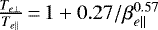
Possible instability mechanisms are examined in Figs. 6. The most striking feature is that the waves occur when βe∥ > 1. Many of the largest amplitude waves occurred in Encounter 4, which had significantly higher βe∥. Halekas et al. (2020a) show that during encounters 1 and 2 inside 0.24 AU, βe∥ was usually <1. This association of narrowband whistler waves with βe∥ > 1 was also seen in the STEREO data at 1 AU. The wave occurrence is constrained by both the whistler temperature anisotropy threshold and the heat flux fan instability threshold, as was also the case at 1 AU (Cattell et al. 2020).The temperature anisotropy destabilizes parallel propagating waves at lower frequencies that we observe. We conclude, therefore, that the waves are most likely driven by the fan instability. This is consistent with the study of the electron heat flux and beta for all intervals inside 0.25 AU in the first five encounters by Halekas et al. (2020b), and with the conclusion of Agapitov et al. (2020) for a set of events in Encounter 1. We note, however, that there are a significant number of cases with large βe∥ where the normalized heat flux is above the threshold (most are from Encounter 4).
The third panel of Fig. 6 plots the energy associated with the electron Alfvén speed for the whistler events for comparison to the electron beam driven instability proposed by Sauer & Sydora (2010). This mechanism, which generates highly oblique waves, requires electron beams that propagate at speeds greater than twice the electron Alfvén speed. The energy associated with the Alfvén speed is very low for the whistler events, ~10–20 eV; thus this mechanism would require beams with energies of ~40–80 eV. This is an order of magnitude lower than would be required for the mechanism to operate at 1 AU. To date, we have not yet been able to identify beam features at the appropriate energies in either event list.
To better assess the occurrence probability of these waves, we utilized one electric field channel in the DC coupled spectral data at 30 s resolution. We examined by eye the spectral data for each hour during the first encounter interval shown in the BPF data in Fig. 1, which covers 31 h on November 2 and 3. This yields only a very rough estimate of the occurrence rate. The individual waveform captures (duration 3.5 s) usually contain several individual wave packets. An example of a 3.5 s waveform capture was shown above in Fig. 1, packet #4. The large amplitude whistler packets have durations on the order of a few seconds (see #4, and the shorter duration waveforms in Fig. 1), while the lower amplitude waves can last through an entire capture. Waveform #1 in Fig. 1 provides an example when the higher frequency Bernstein waves had the largest amplitude for the initial ~1 s, followed by an interval with both wave types with whistler dominating from ~1 to 2 s. We also examined the higher cadence BPF data, which can more accurately determine the duration of regions with whistler packets. The BP cadence is comparable to the duration of the observed large amplitude whistler packets. A comparison of the spectral (1 sample/64 Cy) to the BPF data (1 sample/2 Cy) suggests that the occurrence could be on the order of five to ten percent, based on the electric field spectra.There are a significant number of waves that are only observed in the electric field, which is consistent with very oblique propagation. Any definitive determination of an occurrence rate will depend on the amplitude threshold selected.
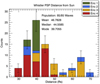 |
Fig. 2 Number of narrowband whistler wave captures color coded by encounter number. The number was not normalized by the total number of waveform captures obtained. |
Average, minimum, and maximum values of parameters for Encounters 1 through 4.
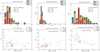 |
Fig. 3 Spacecraft frame frequencies for narrowband whistler wave captures color coded by encounter. Top: number of events versus frequency, frequency normalized by electron cyclotron frequency, and magnitude of the background magnetic field. Bottom: whistler event frequency, frequency normalized by electron cyclotron frequency, and background magnetic field versus radial distance from the Sun. |
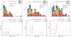 |
Fig. 4 Whistler peak amplitudes color coded by encounter. Left panels: number of whistler captures versus amplitude of electric field, magnetic field, and magnetic field normalized by background magnetic field. Right panels: event amplitude of electric field, magnetic field, and magnetic field normalized by background magnetic field versus radial distance from the Sun. |
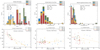 |
Fig. 5 Whistler dependence on core density, core, and suprathermal temperature (from the QTN measurement). Top panels: plot the number of events versus core electron density, core, and suprathermal temperature. Bottom panels: plot the same quantities versus radial distance from the Sun. |
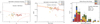 |
Fig. 6 Comparison to instability mechanisms. From left to right: temperature anisotropy versus parallel electron beta for wave events. The upper red line is the whistler temperature anisotropy threshold, |
4 Discussion and conclusions
We have compared statistics of the properties of the narrowband whistler-mode waves observed in waveform capture data from PSP during the first four encounters inside ~0.3 AU to properties observed in waveform capture data from STEREO at 1 AU. At both radial distances, the waves are narrowband and large amplitude. The association with heat flux and beta is generally consistent with the whistler fan instability. In both data sets, the whistlers are only observed for beta >1, and the average temperature anisotropy was ~0.9. The PSP electron data show significant scattering at strahl energies, as is documented in detail by Cattell et al. (2021). This is consistent with a study of electron heat flux (Halekas et al. 2020b) for Encounters 1 through 5, which shows that the heat flux and beta were constrained by the fan instability threshold, providing evidence that these waves regulate the electron heat flux.
Many instability mechanisms have been proposed for whistler-mode waves in the solar wind that have free energy sources associated with electron properties, including electron temperature anisotropies (Gary & Wang 1996), heat flux (Feldman et al. 1975; Gary et al. 1994), heat flux fan instability (Krafft & Volokitin 2010; Vasko et al. 2019), the fast magnetosonic-whistler mode (Verscharen et al. 2019), and electron beam instability (Sauer & Sydora 2010). Theoretical studies of the dispersion relations have concluded that the most unstable modes for the temperature anisotropy and heat flux instabilities are parallel propagating, and they have frequencies f/fce of ~.01, which are lower than the frequencies we observe. The transition to oblique modes (Gary et al. 2011) occurs at values of beta that are much smaller than those observed in the PSP data presented herein. Only the heat flux fan instability, the magnetosonic-whistler mode, and the beam instability have the highest growth rates at oblique angles. The PSP whistlers occurred when beta was high, and the events for which Doppler shifts could be determined had frequencies of f∕fce of ~0.2. Most cases, however, propagated within 20 degrees of the magnetic field, and none were propagating close to the resonance cone as was seen by Agapitov et al. (2020) in a study of lower frequency whistlers in Encounter 1 and by Cattell et al. (2020) at 1 AU. The magnetosonic-whistler mode is low beta, and the most unstable modes are at higher frequencies (f/fce ~ 0.5) than observed at PSP (Verscharen et al. 2019). No beam features have been observed in the energy range needed for the whistler beam instability. The whistler fan instability is most unstable in the range of f∕fce of ~0.1 to 0.2 (Vasko et al. 2019), which is the range we observe. As shown in Fig. 7, the wave occurrence was constrained by the heat fan flux instability threshold. For these reasons, we conclude that the whistler-mode waves observed by PSP are most likely due to the fan instability, as was also the case for the STEREO whistlers (Cattell et al. 2020). Although the wave occurrence is also constrained by whistler temperature anisotropy, the observed wave properties are not usually consistent with this mode. As discussed below, however, it may be the case that the parallel whistlers and the very oblique whistlers are associated with different instability or saturation mechanisms.
At 1 AU, two distinct populations of whistler-mode waves with frequencies of f∕fce of ~0.1 to .2 have been reported from waveform capture data; one population is parallel-propagating with small electric field amplitudes (Lacombe et al. 2014; Graham et al. 2017; Tong et al. 2019) and one is obliquely propagating with resultant large electric fields (Breneman et al. 2010; Cattell et al. 2020). Although the parallel-propagating waves are usually seen in quiet, slow solar wind (Lacombe et al. 2014), Tong et al. (2019) show that quasi-parallel whistlers can also occur in the faster solar wind. The oblique waves are often seen in faster solar wind (Breneman et al. 2010; Cattell et al. 2020) (see Fig. 7). The PSP data shown herein include both parallel and oblique waves, as is also described in Agapitov et al. (2020). There is a tendency for more electrostatic whistlers (i.e., more oblique) to occur within regions of enhanced flow. A recent study of frequency bank spectral data from Helios (Jagarlamudi et al. 2020) presented statistics on waves with spacecraft frame frequencies between ~ flh and 0.5 fce, identified in the search coil magnetic field data at distances of 0.3–0.9 AU. The observed spectral peaks were identified aswhistler-mode based on similarities to Lacombe et al. (2014), but the polarization, wave vectors, and Doppler shifts could not be determined. The waves were observed almost exclusively in the slow solar wind (<400 km s−1).
Figure 7 plots histograms of the number of whistler events versus the solar wind speed in the Cattell et al. (2020) STEREO database (left) and the number of PSP events color coded by the encounter (right) versus solar wind speed. The center panel plots the PSP events versus the solar wind speed and radial distance. The highly oblique whistlers observed at 1 AU by STEREO are predominantly seen with solar wind speeds of ~400 km s−1, but they are also observed with speeds up to ~700 km s−1. PSP eventsare associated with lower solar wind speeds (~300 km s−1). The bi-modal distribution is likely due to the small number of events and to radial distance effects as well as differences in conditions during each encounter, as indicated by the center panel which plots the PSP events versus the solar wind speed and radial distance. Encounter 4 events were all obtained inside ~50 solar radii and solar wind speeds were ~200 km s−1, whereas events during Encounters 2 and 3 were primarily outside ~50 solar radii with solar wind speeds of ~350 km s−1 (see also Table 1). The contrast in solar wind conditions and heat flux during Encounter 4 compared to Encounters 1 and 2 is described by Halekas et al. (2020b). The differences in wave association with the solar wind speed between PSP events inside .3 AU and the STEREO events at 1 AU may just be due to the evolution of the solar wind. The Jagarlamudi et al. (2020) observations which cover the distances between 0.3 and 0.9 AU, however, were associated with slow flow. Wave vector angles have been determined for only a small fraction of the PSP events; therefore, it is not yet possible to determine if there is a relationship between wave obliquity and solar wind speed at these radial distances. The parallel propagating waves and the oblique waves may represent two different modes or, alternatively, different sources of free energy. However, the distinction may also be due to differences in instrumentation. Future studies utilizing the PSP data set may resolve the relationship between the parallel and highly oblique waves.
There are two main differences between the characteristics of the whistlers identified in waveform captures inside 0.2 AU and the waves at 1 AU: (1) the association with larger scale solar wind properties and structure; and (2) the occurrence of a broader band less coherent mode at 1 AU which has not been identified yet in PSP waveform data. In addition, inside 0.2 AU, the narrowband electromagnetic whistlers are interspersed with lower amplitude electrostatic whistler-mode waves and Bernstein waves at frequencies of ~0.7 fce to > fce (Malaspina et al. 2020; Bale et al. 2019), which have not been observed at 1 AU in the STEREO waveform data.
At 1 AU, the narrowband oblique whistlers are most often associated with SIRs, frequently filling the downstream region of increased solar wind speed and usually variable magnetic field. The waves are also seen within CMEs (Cattell et al. 2020). As shown in Fig. 1, inside ~0.3 AU, the whistlers are associated with intervals of variable background magnetic field and slight increases in solar wind flow, sometimes due to magnetic field switchbacks. The association with switchbacks has been previously described by Agapitov et al. (2020). The intervals with packets of narrowband whistlers can last for several hours, but not for a day or more as seen at 1 AU. This is most likely due to the much more variable solar wind conditions observed by PSP close to the Sun. Future studies including data from additional encounters will examine whether there is an association between the whistlers with SIRs or CMEs inside ~0.3 AU.
Both the wave magnetic field amplitudes normalized to the background magnetic field and the electric field amplitudes observed by PSP decrease with radial distance from the Sun, however, the average electric field amplitudes observed by STEREO at 1 AU are comparable to those seen by PSP near 0.3 AU. This may be due to the different selection criteria for burst data for the two spacecrafts or to differences in the physics. For example, the waves may, on average, be more oblique at 1 AU or the wave growth and saturation mechanisms may be different due to differences in the solar wind and electron properties.
Initial results on whistler-mode waves observed by PSP identified in the magnetic field data during the first encounter have been presented by Agapitov et al. (2020), utilizing the ~300 samples s−1 waveform data. The observed waves had large amplitudes (~2–4 nT), had variable wave angles, and were often propagating sunward. The waves were significantly Doppler shifted resulting in plasma frame frequencies of ~0.2–0.5 fce. The differences including average f∕fce warrant additional studies for other encounters. This will require developing a method to accurately determine the wave vector direction when only two components of the search coil data are available, utilizing an approach similar to that used on STEREO based on the three components of the electric field waveform and the cold plasma dispersion relation (Cattell et al. 2008).
In conclusion, we have shown that narrowband whistler mode waves observed in the PSP waveform capture data inside ~0.3 AU have many characteristics similar to those seen by STEREO at 1 AU. In both regions, the waves are most consistent with the whistler heat flux fan instability and occur when beta is greater than 1. The waves at 1 AU have slightly higher average f∕fce and are on average more oblique, but both of these differences may be due to the small number of PSP events for which we have determined wave angle and Doppler shifts. When there are wave events, the radial dependence of the core and suprathermal temperatures is different from that seen for the full electron data set (Halekas et al. 2020a), possibly indicating that the waves heat core electrons. At PSP, the waves are often associated with regions of variable magnetic field and slightly enhanced solar wind flow, and sometimes with “switchbacks”, whereas at 1 AU, the waves are most often seen in the downstream region of SIRs, which are also regions of enhanced flow. Inside ~0.3 AU, the regions containing wave packets tend to last for intervals of hours, whereas at 1 AU, they can last for days. It is very likely that these differences are due to the fact that the solar wind is much more variable on short time scales at PSP compared to at 1 AU. The waves are associated with scattering of strahl energy electrons. A very rough estimate of the wave occurrence at PSP suggests that the waves are often the dominant wave mode at frequencies below ~3 kHz; combined with the observations of scattering, this suggests that the narrowband whistlers may play a significant role in the evolution of solar wind electrons and regulation of heat flux.
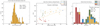 |
Fig. 7 The relationship of whistler occurrence to solar wind speed on PSP and STEREO. From left to right: number of events versus solar wind speed on STEREO from the Cattell et al. (2020) database, PSP whistler events versus the solar wind velocity and radial distance, and the number of PSP whistler events versus the solar wind speed. |
Acknowledgements
We acknowledge the NASA Parker Solar Probe Mission, and the FIELDS team led by S. D. Bale, and the SWEAP team led by J. Kasper for use of data. The FIELDS experiment on the Parker Solar Probe spacecraft was designed and developed under NASA contract NNN06AA01C. Work at University of Minnesota and at University of Iowa was supported under the same contract.
References
- Agapitov, O. V., de Wit, T. D., Mozer, F. S., et al. 2020, ApJ, 891, L20 [Google Scholar]
- Bale, S., Goetz, K., Harvey, P., et al. 2016, Space Sci. Rev., 204, 49 [Google Scholar]
- Bale, S. D., Badman, S. T., Bonnell, J. W., et al. 2019, Nature, 576, 237 [Google Scholar]
- Breneman, A., Cattell, C., Schreiner, S., et al. 2010, J. Geophys. Res. Space Phys., 115, A8 [Google Scholar]
- Case, A. W., Kasper, J. C., Stevens, M. L., et al. 2020, ApJS, 246, 43 [Google Scholar]
- Cattell, C., Wygant, J. R., Goetz, K., et al. 2008, Geophys. Res. Lett., 35, 1 [Google Scholar]
- Cattell, C., Short, B., Breneman, A., & Grul, P. 2020, ApJ, 897, 126 [Google Scholar]
- Cattell, C., Breneman, A., Dombeck, J., et al. 2021, ApJ, 911, L29 [Google Scholar]
- Feldman, W. C., Asbridge, J. R., Bame, S. J., Montgomery, M. D., & Gary, S. P. 1975, J. Geophys. Res., 80, 4181 [Google Scholar]
- Gary, S. P., & Wang, J. 1996, J. Geophys. Res. Space Phys., 101, 10749 [Google Scholar]
- Gary, S. P., Scime, E. E., Phillips, J. L., & Feldman, W. C. 1994, J. Geophys. Res. Space Phys., 99, 23391 [Google Scholar]
- Gary, S. P., Neagu, E., Skoug, R. M., & Goldstein, B. E. 1999, J. Geophys. Res., 104, 19843 [Google Scholar]
- Gary, S. P., Liu, K., & Winske, D. 2011, Phys. Plasmas, 18, 082902 [Google Scholar]
- Graham, G., Rae, I., Owen, C., et al. 2017, J. Geophys. Res. Space Phys., 122, 3858 [Google Scholar]
- Halekas, J., Whittlesey, P., Larson, D., et al. 2020a, ApJS, 246, 22 [Google Scholar]
- Halekas,J. S., Whittlesey, P. L., Larson, D. E., et al. 2020b, A&A, 650, A15 (PSP SI) [Google Scholar]
- Jagarlamudi, V. K., Alexandrova, O., Berčič, L., et al. 2020, ApJ, 897, 118 [Google Scholar]
- Kasper, J. C., Abiad, R., Austin, G., et al. 2016, Space Sci. Rev., 204, 131 [NASA ADS] [CrossRef] [Google Scholar]
- Kasper, J., Bale, S., Belcher, J., et al. 2019, Nature, 576, 228 [Google Scholar]
- Krafft, C., & Volokitin, A. 2010, Phys. Plasmas, 17, 102303 [Google Scholar]
- Lacombe, C., Alexandrova, O., Matteini, L., et al. 2014, ApJ, 796, 5 [Google Scholar]
- Maksimovic, M., Zouganelis, I., Chaufray, J.-Y., et al. 2005, J. Geophys. Res. Space Phys., 110, A9 [Google Scholar]
- Malaspina, D. M., Ergun, R. E., Bolton, M., et al. 2016, J. Geophys. Res. Space Phys., 121, 5088 [Google Scholar]
- Malaspina, D. M., Halekas, J., Berčič, L., et al. 2020, ApJS, 246, 21 [Google Scholar]
- Moncuquet, M., Meyer-Vernet, N., Issautier, K., et al. 2020, ApJS, 246, 44 [Google Scholar]
- Sauer, K., & Sydora, R. D. 2010, Ann. Geophys., 28, 1317 [Google Scholar]
- Štverák, Š., Maksimovic, M., Trávníček, P. M., et al. 2009, J. Geophys. Res. Space Phys., 114 [Google Scholar]
- Tong, Y., Vasko, I. Y., Artemyev, A. V., Bale, S. D., & Mozer, F. S. 2019, ApJ, 878, 41 [Google Scholar]
- Vasko, I., Krasnoselskikh, V., Tong, Y., et al. 2019, ApJ, 871, L29 [Google Scholar]
- Verscharen, D., Chandran, B. D. G., Jeong, S.-Y., et al. 2019, ApJ, 886, 136 [Google Scholar]
- Whittlesey, P. L., Larson, D. E., Kasper, J. C., et al. 2020, ApJS, 246, 74 [Google Scholar]
- Wilson III, L. B., Chen, L.-J., Wang, S., et al. 2019, ApJS, 245, 24 [Google Scholar]
All Tables
All Figures
|
Fig. 1 Interval during Encounter 1 with narrow band whistler-mode waves and higher frequency electrostatic waves. Left panels: DC-coupled BPF electric field spectrum from 12 to 4000 Hz; DC-coupled BBF magnetic field from 12 to 4000 Hz; magnetic field in RTN coordinates, R component of magnetic field in red with radial component of ion flow −300 km s−1 in blue. Pitch angle spectra for electrons with center energy of 314 and 204 eV. Units for the wave spectra are volts and nT, and for the electron data are eV cm−2 s. Right panels: spacecraft x component of the electric field (in mV m−1) snapshots from seven different waveform captures during this interval at approximate times indicated by arrows with blue arrows indicating more than one snapshot. We note that the time durations vary. See text for details. |
| In the text | |
|
Fig. 2 Number of narrowband whistler wave captures color coded by encounter number. The number was not normalized by the total number of waveform captures obtained. |
| In the text | |
|
Fig. 3 Spacecraft frame frequencies for narrowband whistler wave captures color coded by encounter. Top: number of events versus frequency, frequency normalized by electron cyclotron frequency, and magnitude of the background magnetic field. Bottom: whistler event frequency, frequency normalized by electron cyclotron frequency, and background magnetic field versus radial distance from the Sun. |
| In the text | |
|
Fig. 4 Whistler peak amplitudes color coded by encounter. Left panels: number of whistler captures versus amplitude of electric field, magnetic field, and magnetic field normalized by background magnetic field. Right panels: event amplitude of electric field, magnetic field, and magnetic field normalized by background magnetic field versus radial distance from the Sun. |
| In the text | |
|
Fig. 5 Whistler dependence on core density, core, and suprathermal temperature (from the QTN measurement). Top panels: plot the number of events versus core electron density, core, and suprathermal temperature. Bottom panels: plot the same quantities versus radial distance from the Sun. |
| In the text | |
|
Fig. 6 Comparison to instability mechanisms. From left to right: temperature anisotropy versus parallel electron beta for wave events. The upper red line is the whistler temperature anisotropy threshold, |
| In the text | |
|
Fig. 7 The relationship of whistler occurrence to solar wind speed on PSP and STEREO. From left to right: number of events versus solar wind speed on STEREO from the Cattell et al. (2020) database, PSP whistler events versus the solar wind velocity and radial distance, and the number of PSP whistler events versus the solar wind speed. |
| In the text | |
Current usage metrics show cumulative count of Article Views (full-text article views including HTML views, PDF and ePub downloads, according to the available data) and Abstracts Views on Vision4Press platform.
Data correspond to usage on the plateform after 2015. The current usage metrics is available 48-96 hours after online publication and is updated daily on week days.
Initial download of the metrics may take a while.