| Issue |
A&A
Volume 650, June 2021
|
|
|---|---|---|
| Article Number | A63 | |
| Number of page(s) | 7 | |
| Section | Extragalactic astronomy | |
| DOI | https://doi.org/10.1051/0004-6361/202038438 | |
| Published online | 08 June 2021 | |
Less and more IGM-transmitted galaxies from z ∼ 2.7 to z ∼ 6 from VANDELS and VUDS⋆,⋆⋆
1
European Southern Observatory, Av. Alonso de Córdova 3107, Vitacura, Santiago, Chile
e-mail: This email address is being protected from spambots. You need JavaScript enabled to view it.
2
INAF – Osservatorio Astronomico di Roma, Via Frascati 33, 00078 Monteporzio Catone, Italy
3
Aix Marseille Université, CNRS, LAM (Laboratoire d’Astrophysique de Marseille) UMR 7326, 13388 Marseille, France
4
INAF – Osservatorio di Astrofisica e Scienza dello Spazio, Via Gobetti 93/3, 40129 Bologna, Italy
5
INAF – Osservatorio Astrofisico di Arcetri, largo E. Fermi 5, 50125 Firenze, Italy
6
INAF-Astronomical Observatory, Via G.B. Tiepolo 11, 34143 Trieste, Italy
7
IFPU – Institute for Fundamental Physics of the Universe, Via Beirut 2, 34151 Trieste, Italy
8
INAF IASF-Milano, Via A.Corti 12, 20133 Milano, Italy
9
University of Bologna – Department of Physics and Astronomy, Via Gobetti 93/2, 40129 Bologna, Italy
10
Instituto de Investigación Multidisciplinar en Ciencia y Tecnología, Universidad de La Serena, Raúl Bitrán 1305, La Serena, Chile
11
Departamento de Astronomía, Universidad de La Serena, Av. Juan Cisternas 1200 Norte, La Serena, Chile
12
AIM, CEA, CNRS, Université Paris-Saclay, Université Paris Diderot, Sorbonne Paris Cité, 91191 Gif-sur-Yvette, France
13
Centre for Astrophysics Research, University of Hertfordshire, Hatfield AL10 9AB, UK
14
Cosmic DAWN Center, Vibenshuset, Lyngbyvej 2, 2100 Copenhagen, Denmark
15
Niels Bohr Institute, Copenhagen University, Lyngbyvej 2, 2100 Copenhagen O, Denmark
16
Space Telescope Science Institute, 3700 San Martin Drive, Baltimore, MD 21218, USA
17
Max-Planck-Institut für Astronomie, Königstuhl 17, 69117 Heidelberg, Germany
18
Department of Physics, University of California, Davis, One Shields Ave., Davis, CA 95616, USA
19
Observatoire de Genève, Université de Genève, 51 Ch. des Maillettes, 1290 Versoix, Switzerland
Received:
18
May
2020
Accepted:
18
February
2021
Abstract
Aims. Our aim is to analyze the variance of the intergalactic medium (IGM) transmission by studying this parameter in the rest-frame UV spectra of a large sample of high-redshift galaxies.
Methods. We made use of the VIMOS Ultra Deep Survey and the VANDELS public survey to gain insight into the far UV spectrum of 2.7 < z < 6 galaxies. Using the SPARTAN fitting software, we estimated the IGM toward individual galaxies and then divided them into two sub-samples characterized by a transmission above or below the theoretical prescription. We created average spectra of combined VUDS and VANDELS data for each set of galaxies in seven redshift bins.
Results. The resulting spectra clearly exhibit the variance of the IGM transmission that can be seen directly from high-redshift galaxy observations. Computing the optical depth based on the IGM transmission, we find an excellent agreement with results for quasi-stellar objects. In addition, our measurements appear to suggest that there is a large dispersion of redshift where a complete Gunn-Peterson Trough occurs, depending on the line of sight.
Key words: intergalactic medium / galaxies: high-redshift / cosmology: miscellaneous
VANDELS: based on observations made with ESO Telescopes at the La Silla or Paranal Observatories under programme ID(s) 194.A-2003.
VUDS: based on data obtained with the European Southern Observatory Very Large Telescope, Paranal, Chile, under Large Program 185.A-0791.
Deceased.
© ESO 2021
1. Introduction
The light coming from distant sources (e.g., quasi-stellar objects and galaxies) is absorbed by the gaseous hydrogen systems that lie along the line of sight. At increasing redshift, this effect, called intergalactic medium (IGM) absorption, can be so strong that all the light at wavelengths blueward the Lyman α (Lyα) at 1216 Å becomes invisible to us. This absorption has been the topic of numerous studies and is mainly connected with the growth of the large-scale structure as predicted by the hierarchical structure formation scenario. It is also tightly connect with the epoch of reionization (e.g., Cen et al. 1994).
Twenty five years ago, Madau (Madau 1995, hereafter M95) proposed a theoretical model able to reproduce the shape of the extinction curve as a function of redshift. Using this model, the author concluded that the IGM transmission, Tr(Lyα), decreases with increasing redshift and that the scatter at a given redshift should be large, for example, from 20% to 70%, with an average of 40% at z = 3.5. A decade later, Meiksin (Meiksin 2006, hereafter M06) produced an update of this model using the Λ cold dark matter cosmological predictions. More recently, Inoue et al. (2014) developed a new transmission model. This predicts a weaker average absorption in the range z = 3–5, but the absorption becomes stronger at z > 6. On the observational side, studies of the IGM have been focused almost exclusively on quasi-stellar objects (QSOs). Faucher-Giguère et al. (2008) used 86 high-resolution quasar spectra with a high signal-to-noise ratio (S/N) to provide reference measurements of the dispersion over 2.2 < z < 4.6. Dall’Aglio et al. (2008) used 40 bright quasars to produce the measurements of the IGM optical depth between z = 2.5 and z = 4.5, while Becker et al. (2013) extended the redshift range up to 5.5 with more than 6000 quasars. They all found that the transmission indeed decreases with increasing redshift.
Until a few years ago, no observational studies were made of the evolution of the IGM transmission from galaxy samples mainly because of the lack of large spectroscopic samples with high signal-to-noise ratios at high redshift that probed a wavelength range between the Lyman-limit at 912 Å and Lyα. Hence, the IGM transmission toward extended galaxies has so far not been compared with the well-known results for point-like QSO samples. In two recent papers we were able to compute the IGM transmission for a large sample of galaxies using the VIMOS Ultra Deep Survey (VUDS; Le Fèvre et al. 2015; Thomas et al. 2017, hereafter T17) and the VANDELS survey (McLure et al. 2018; Pentericci et al. 2018; Thomas et al. 2020, hereafter T20). In these studies we showed that not only can we measure the IGM transmission using galaxy spectra, but that it is crucial for understanding how galaxies are selected with Lyman-break techniques (Steidel et al. 1995), which highly depend on the IGM.
In this paper, we have assembled more than 2500 galaxies from VUDS and VANDELS at z > 2.7 with measured IGM absorption to create averaged IGM spectra in different redshift bins to study the IGM extinctions and visually determine the effect of the IGM variance on galaxy data. We describe the VUDS and VANDELS galaxy sample and selection in Sect. 2. The fitting method with the SPARTAN tool (Thomas 2021) and the recipe we used to compute the IGM are described in Sect. 3. The results are presented in Sect. 4. Finally, we discuss the results in Sect. 6.
All magnitudes are given in the AB system (Oke & Gunn 1983), and we use a cosmology with ΩM = 0.3, ΩΛ = 0.7, and h = 0.7.
2. Data
We use deep spectra collected by the VUDS (Le Fèvre et al. 2015) and VANDELS (McLure et al. 2018; Pentericci et al. 2018). We briefly describe both surveys and refer to the survey description papers for more details. Both surveys have been carried out with the now-decommissioned VIsible Multi-Object Spectrograph (VIMOS) instrument installed at the Nasmyth focus of Unit Telescope 3 of the Very Large Telescope.
VUDS (P.I. O. Le Fèvre) is a European Southern Observatory (ESO) large program designed to study the first billion years of galaxy evolution. It is based on the observation of 10 000 sources up to z = 6.5 selected primarily with the photometric redshift method performed with the LePhare software (Arnouts et al. 1999; Ilbert et al. 2006). Each target was observed for a total of ∼14h in the wavelength range 3500 ≤ λ ≤ 9350 Å using the two low-resolution grisms of the instrument at R ∼ 240. The data reduction was carried out using the VIPGI software (Scodeggio et al. 2005). As the targets are in well-known fields (VIMOS VLT Deep Survey [VVDS] 2h field, Cosmic evolution Survey [COSMOS] and Extended Chandra Deep Field South [ECDFS]), a large number of multiwavelength photometric data are available to complement the spectroscopic information. We refer to Le Fèvre et al. (2015) for a full description of the survey.
The second sample comes from the VANDELS survey (P.Is R. McLure and L. Pentericci). VANDELS is an ESO public spectroscopic survey aiming at the exploration of the high-redshift Universe at 1 < z < 7. More than 2100 galaxies have been observed using the VIMOS medium-resolution grism at R ∼ 600 from 4800 to 10 000 Å, and the exposure time varied from 20 h up to 80 h. As for VUDS, most targets were selected using the photometric redshift technique. The data reduction was carried out using the EASYLIFE package (Garilli et al. 2012). Targets were selected in the two widely observed ultra deep survey [UDS] and Chandra deep field south [CDFS] fields, which allows the association of the spectroscopy to a large number of multiwavelength photometric data. The survey is described by McLure et al. (2018), Pentericci et al. (2018) and the final data release is presented in Garilli et al. (2021).
For both surveys, all the redshift estimates were performed using the EZ software (Garilli et al. 2010), a template cross-correlating code, and they both use an equivalent redshift flag system to assess the quality of the redshift measurements. In this scheme, galaxies with a redshift flag 2, 3, and 4 are those with the most reliable redshift measurements, with a probability to be correct of 75%, 95%, and 100%, respectively.
In this study, we are interested in galaxies with IGM transmissions that are higher and lower than the mean theoretical transmission. As defined in T17 and T20, this quantity is measured between rest-frame 1070 Å and 1170 Å. This requirement imposes a lower redshift limit of z = 3.7 for VANDELS (taking a lower wavelength of ∼5000 Å) and z = 2.7 for VUDS (lower wavelength at ∼3900 Å). Finally, we selected only galaxies with a redshift flag of 2, 3, or 4, which ensures that the objects have the best-quality redshift. This leads to a combined sample of 2502 galaxies, including 296 galaxies from VANDELS and 2206 galaxies from VUDS. As the goal is to analyze galaxy spectra, it is worth mentioning that VANDELS spectra were rebinned to match the VUDS wavelength grid.
3. Method: SPARTAN tool and IGM estimation
The IGM transmission was estimated using the software called spectroscopic and photometric fitting tool for astronomical analysis (SPARTAN, Thomas 2021). This is a Python-based software created to be able to fit both photometry and spectroscopy in a common environment. We provide in this section the relevant aspects for this paper. SPARTAN uses a χ2 minimization technique that consists of a comparison of the observations to theoretical galaxy models (see T20 for more details).
In order to select galaxies on the basis of their estimated IGM transmission, we need to measure this transmission. This is done through the two-step template fitting method described in T20, which allows reducing the degeneracy between dust extinction and IGM absorption. The first step is to estimate the dust attenuation parameter E(B − V)s based on the SPARTAN fitting of all the photometric data points. The second step is fixing the dust extinction (from the first pass) on the spectral data, which provides the IGM transmission. The fitting is done using Bruzual & Charlot (2003) models with a Chabrier (2003) initial mass function. The stellar-phase metalicity ranges from subsolar (0.2Z⊙ and 0.4Z⊙) to solar (1.0Z⊙). We assumed an exponentially delayed star formation history of the form SFR ∝ t × τ−2 × exp(−t/τ) with a timescale parameter, τ, ranging from 0.1 Gyr to 2.0 Gyr. The ages (corresponding to the time since the onset of star formation) range from 0.01 Gyr to 4 Gyr. It is worth noting that this range of ages is further limited by the age of the Universe at the redshift that is considered during the fit. For the photometric fitting, the E(B − V)s parameter can vary from 0.0 to 0.39 (in 0.03 steps). As described above, this parameter is fixed during the second pass spectral fitting. Finally, the IGM prescription that we used is from T17, in which we built IGM transmission templates around the mean of M06. At a given redshift, six empirical additional curves at ±0.5σ, ±1.0σ, and ±1.5σ were created. This allows us to use the IGM as a free parameter in our fit and to explore a wide range of IGM transmissions. At z = 3, the IGM transmission, Tr(Lyα), can range from 20% to 100%, while at z = 5, it might vary from 5% to 50%. The Lyα transmission is estimated directly on these models as the average of the selected model between 1070 Å and 1170 Å (we refer to T20 for examples of spectral fitting).
4. More and less IGM-transmitted galaxies at z > 2.7
The objective of this paper is to study the galaxies in different redshift bins whose IGM transmission is different from the theoretical mean. In order to achieve this goal, we created average spectra of galaxies selected based on their IGM transmission computed from the SPARTAN fitting. This was done in seven redshift bins, 2.7 ≤ z < 3.0, 3.0 ≤ z < 3.3, 3.3 ≤ z < 3.6, 3.6 ≤ z < 4.0, 4.0 ≤ z < 4.5, 4.5 ≤ z < 4.8, and z > 4.8. The choice of these seven bins was a trade-off between maximizing the number of points and keeping a high number of galaxies so that the S/N would be high enough for our study, nevertheless, It is worth mentioning that the change of this binning, e.g. with less bins, does not change our results. The galaxies in each bin were separated into two subsamples: the more transmitted galaxies, that is, those whose measured IGM transmission is higher than the predicted mean of the M06 prescription (with a selected model at ≥0.5σ, see previous section), and the less transmitted galaxies, that is, those whose measured IGM transmission is lower than the mean of the M06 prescription (with a selected model at ≤0.5σ). For each set of galaxies we created an average spectrum using the specstack1 tool (Thomas 2019a). The tool works as follows. For a given set of galaxies, we deredshift all the individual spectra and normalized them in a region redward of the Lyα line (in our case, 1345 Å–1380 Å because this region lacks spectral features). Then we regridded the spectra in a common wavelength grid. Finally, at a given wavelength, we computed the average of the entire flux density in each given pixel weighted by the individual S/N of the spectra using a 3σ sigma-clipping method. In the seven redshift bins, the resulting average spectra based on our 2502 galaxies from both VUDS and VANDELS are presented in Fig. 1 and their associated data are displayed in Table 1. The averaged spectra were computed between 912 Å and 1500 Å rest frame. In each redshift bin we show three average spectra: an average spectrum made from the more IGM-transmitted galaxies, an average spectrum made from the less IGM-transmitted galaxies, and finally, an average spectrum made from all the galaxies available in the considered redshift bin independent of the IGM transmission2.
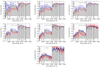 |
Fig. 1. Average spectra with different IGM-attenuated samples. All spectra are given in the restframe (rf). We show seven different redshift bins (from top left to bottom left): 2.7 < z < 3.0, 3.0 < z < 3.3, 3.3 < z < 3.6, 3.6 < z < 4.0, 4.0 < z < 4.5, 4.5 < z < 4.8, and z > 4.8. For each panel we show the averaged spectrum for the more transmitted galaxies in blue, the averaged spectrum of the less transmitted galaxies in red, and the averaged spectrum of all the galaxies in gray. |
First of all, it is important to note that 70% of the average spectra are made of more than 100 individual spectra. The other 30% are average spectra at the highest redshift bins, where we have fewer spectra. As a result, the latter have a higher level of noise.
In each redshift bin, the average redshift of that comprise the three composite spectra are similar, and it is therefore meaningful to compare them directly. Very importantly, Fig. 1 shows that redward of the Lyα line, the spectra of the three samples are very close to each other, which means that the underlying galaxy populations are similar, and more notably, that the dust properties are similar. Therefore the strong flux variation below the Lyα line primarily depends on the IGM extinction along the line of sight. At every redshift, the less transmitted sample is much dimmer at 1070 Å–1170 Å than the more transmitted sample, except for the highest redshift spectra (see next section). Based on the measurement on the average spectra, the flux density at 1070 Å–1170 Å of less transmitted galaxies is fainter on average by 40% than that of more transmitted galaxies. This difference has a strong effect on the selection of galaxies based on the Lyman-break technique (as shown in T17 at z ∼ 3.2 with ugr colour-colour diagram). However, we note that for the two highest redshift bins, the flux density of the average sample (in gray) is very similar to that of more transmitted sample. In these bins, there are fewer galaxies in the sample that is less transmitting, therefore the average tends to be closer to the more transmitted sample. We investigate the potential origin of this asymmetry in Sect. 6.1. For a better vizualisation, the evolution of the flux itself in this region is displayed in Fig. 2, where all the regions have been redshifted to the average redshift of the bin (see Table 1).
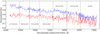 |
Fig. 2. Evolution of the region in which the Lyα transmission is computed (1070–1170 Å) in the different redshift bins of Fig. 1, but this time in the observed frame (the redshifts of the spectra are set to the average redshift of the redshift bin). The vertical dashed lines show the separation between each redshift bin (in the middle of the overlap). The color-coding is the same as in Fig. 1. |
We computed the average flux of the rest-frame stacked spectra in the IGM transmission region (1070–1170 Å), and the evolution of this average flux is shown in Fig. 3. As seen in the stacks, the average flux decreases with redshift, as expected due to the evolution of the IGM (M06 and M95). Nevertheless, the evolution seems to be different for the two samples. We computed the difference in average flux between the more and the less transmitted sample, ΔF. These measurements are reported in the penultimate column of Table 1. The difference decreases with increasing redshift. It changes from 0.37 at z ∼ 2.85 to 0.14 at z ∼ 5.04, indicating that the difference in transmission between the two sets of galaxies is also reduced. We also computed the fractional difference ΔF/⟨Fall⟩ and report it in the last column of Table 1. It slightly decreases with redshift from 0.45 at z ∼ 2.85 to 0.34 at z ∼ 5.04. Nevertheless, the scatter of the points prevents us from drawing any conclusion from this evolution. These evolutions are well fit by a simple linear function, f(z) = a × z + b (valid for taking all the points of Fig. 3 from zsource = 2.85 and zsource = 5.04):
![Mathematical equation: $$ \begin{aligned}&\langle F\rangle _{\rm less} = -0.101[\pm 0.008] \times z + 0.866 [\pm 0.029] \nonumber \\&\langle F\rangle _{\rm more} = -0.181[\pm 0.019] \times z + 1.447 [\pm 0.072] \end{aligned} $$](/articles/aa/full_html/2021/06/aa38438-20/aa38438-20-eq2.gif) (1)
(1)
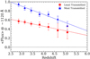 |
Fig. 3. Evolution of the averaged flux in the 1070–1170 Å region in the averaged spectra for the more (in blue) and the less (red) IGM-transmitted average spectra. The two solid lines are linear fits to the evolutions whose functional shapes are given in Eq. (1). |
The fitting method was carried out using the curve_fit function of the scipy.optimize package (Virtanen et al. 2020), which performs a χ2 minimization. The errors on the parameters correspond to the standard deviation estimated from the covariance matrix3.
5. Optical depth
Traditionally, QSO studies compute the HI optical depth from the IGM transmission. This is defined as
 (2)
(2)
where the Tr(Lyα) is the Lyman α transmission computed directly from the IGM template. We applied this transformation to each of our galaxy sets, and the results are reported in Table 2. It is also worth mentioning that QSO studies often use the redshift of the absorbers in the Lyman-α forest, which is defined as:
 (3)
(3)
Optical depth from the IGM transmission in each of our galaxy subsamples.
with zs the redshift of the source and λLyα = 1215.67 Å. To be able to compare our measurements to the QSO literature, we transformed all our redshifts in this section to zabs using λ0 = 1120 Å, the middle of the region in which we measure Tr(Lya).
We compared our estimates to QSO data with data from Dall’Aglio et al. (2008), Faucher-Giguère et al. (2008), Becker et al. (2013, 2015) and the galaxy-based optical depth estimates from Monzon et al. (2020). Our measurements from all our galaxies are in excellent agreement with each of these samples over the whole redshift range. At the high-redshift end of our sample, the scatter of Becker et al. (2015) also reaches our less/more transmitted galaxies. We fit the evolution of the optical depth for each of our samples with an analytical function of the form:
 (4)
(4)
The fit was carried out using the same algorithm as Sect. 4, using the scipy package. We find the following for the three sample:
-
All galaxies: A = 2.655 × 10⁻³ ± 0.001, γ = 3.536 ± 0.170
-
More transmitted: A = 9.540 × 10⁻⁶ ± 6.397 × 10⁻⁶, γ = 6.717 ± 0.413
-
Less transmitted: A = 0.026 ± 0.006, γ = 2.354 ± 0.147
It is worth mentioning that the result of this fit is valid for the redshift range we consider here from zsource = 2.85 to zsource = 5.04.
Finally, the evolution of the optical depth for both more and less transmitted galaxies is well separated at any redshift, which would indicate that some galaxies may become visible below the Lyα line at very different redshifts depending only on their IGM optical depth. At a fixed optical depth, the difference in redshift reaches ≳1.
6. Discussion
6.1. Asymmetry in the distribution of more/less transmitting lines of sight.
As reported in Sect. 4, we observe that in the highest redshift bins, the number of galaxies with an LOS classified as less transmitting is smaller than the number of classified galaxies with an LOS classified as more transmitting. We investigate this asymmetry by looking at the two different surveys independently (see Table 3).
Number of galaxies whose IGM transmission is lower and higher than the theoretical mean from M06.
When the VANDELS survey alone is considered, the distribution of galaxies between less and more transmitting line of sights does not show this asymmetry. On the other hand, when the VUDS data alone are considered, the effect is present. This most probably indicates that the two pass fitting method is not entirely efficient when it is applied to the VUDS data. This may be explained by the the number of points used for the dust estimation using photometric SED-fitting (we used up to 20 bands for VANDELS and around 10 for VUDS). This can be partially resolved by setting lower limits on the photometric fitting, that is, forcing a lower dust attenuation, as shown in T17. This would result in a more symmetric distribution, in the same way as for the VANDELS sources. This action would remove the slight jump that can be seen in Fig. 3 at z > 4 and shift the measurements of the optical depth closer to the Meiksin model (see Fig. 4).
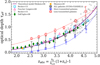 |
Fig. 4. Evolution of the optical depth for each sample of our galaxies and comparison with QSO data. More IGM transmitted galaxies are shown by the blue stars, less transmitted galaxies are shown as red stars, and black star represent the full sample of our galaxies. Dashed lines represent the fit to each sample and are plotted in the same colors. We also show data from the literature with measurements from Dall’Aglio et al. (2008) as green diamonds, from Faucher-Giguère et al. (2008) as pink triangles, from Becker et al. (2013) as light blue squares, and from Becker et al. (2015) as empty gray circles. The orange point is based on galaxy data from Monzon et al. (2020). The solide purple line is the theoretical model from Meiksin (2006). |
6.2. γ values
As shown in the previous section, the fits of Fig. 4 show large differences in the parameters range, especially for the γ parameter which range from 2.354 for the galaxies that are less transmitted to 6.397 for the more transmitting galaxies. In the framework of Lyman-alpha forest studies, the γ parameter is related to the evolution of the number density of Lyα forest clouds with redshift. Press et al. (1993) fit the evolution of the optical depth with a functional of the form τeff(z) = A(1 + z)β, with β = γ + 1. In this case, the β value can be used directly to estimate the evolution of the number of clouds with redshift, which is given by:
 (5)
(5)
In this framework, we must remove 1 to all our values of γ presented in Sect. 5. The γ value is lowest for the less transmitted galaxies. This indicates a slower evolution with redshift. These lines of sight are the most populated by clouds, which leads to a lower transmission. This slower evolution arises because the strong increase in optical depth at high-z (Becker et al. 2015) is less prominent for these line of sights because they are already heavily populated by clouds. In contrast, the more transmitted galaxies are fit with a high γ value, which indicates a strong evolution with redshift. For these galaxies, the lines of sight are less populated by clouds, leading to a higher IGM transmission. The strong evolution of the optical depth at high-z translates into a rapid increase of the number of clouds along the line of sight with redshift for the more transmitted galaxies.
7. Conclusions
Using data from the VUDS and VANDELS programs, we presented the effect of the IGM at redshift z > 2.7. Using averaged spectra, we observed the effect of the IGM for lines of sights that are more and less transmitting that the theoretical average prescription. This leads to two important results:
-
First, the variance of the IGM is clearly visible from galaxy data. The flux for the subsample with the more transmitting lines of sight is higher on average by 63% in the 1070–1170 Å region than the subsample with lower IGM transmission. This has been reported before from the quasar point of view, for instance, by Songaila (2004). From the theoretical point of view, the large variance of the IGM has been shown by Madau (1995), but it has not been emphasized by more recent works. We defer a comprehensive comparison of our galaxy data with simulations to a future study.
-
The estimation of the optical depth from the IGM transmission allowed us to compare our data with multiple QSO studies and shows an excellent agreement. Finally, the observed variance of the IGM described above could lead to different full-opacity redshifts for different categories of lines of sight. The evolution of the optical depth from both more and less attenuated galaxies suggests that galaxies could start to become visible below Lyman-alpha at very different redshifts: at zs ∼ 6.16 for less transmitted galaxies, and at zs ∼ 6.80 for the more transmitted galaxies. Nevertheless, QSO studies at z > 5 indicate that the evolution of the optical depth would become steeper with increasing redshift.
The evolution of the Lyα transmission itself is shown in T20.
Acknowledgments
We wish to thank the anonymous referee for a careful reading of our manuscript and a insightful comments and corrections. We thank the ESO staff for their continuous support for the VANDELS survey, particularly the Paranal staff, who helped us to conduct the observations, and the ESO user support group in Garching. VUDS Data products are made available at the CESAM data center, Laboratoire d’Astrophysique de Marseille, France. RA acknowledges support from FONDECYT Regular Grant 1202007. All the plots have been made using the Photon software (Thomas 2019b) and dfitspy (Thomas 2019c) was used for fits file handling. We would like to dedicate this paper to the memory of Olivier Le Fèvre, PI of the VUDS survey and co-I of the VANDELS survey.
References
- Arnouts, S., Cristiani, S., Moscardini, L., et al. 1999, MNRAS, 310, 540 [NASA ADS] [CrossRef] [Google Scholar]
- Becker, G. D., Hewett, P. C., Worseck, G., & Prochaska, J. X. 2013, MNRAS, 430, 2067 [Google Scholar]
- Becker, G. D., Bolton, J. S., Madau, P., et al. 2015, MNRAS, 447, 3402 [Google Scholar]
- Bruzual, G., & Charlot, S. 2003, MNRAS, 344, 1000 [NASA ADS] [CrossRef] [Google Scholar]
- Cen, R., Miralda-Escudé, J., Ostriker, J. P., & Rauch, M. 1994, ApJ, 437, L9 [Google Scholar]
- Chabrier, G. 2003, PASP, 115, 763 [Google Scholar]
- Dall’Aglio, A., Wisotzki, L., & Worseck, G. 2008, A&A, 491, 465 [NASA ADS] [CrossRef] [EDP Sciences] [Google Scholar]
- Faucher-Giguère, C.-A., Prochaska, J. X., Lidz, A., Hernquist, L., & Zaldarriaga, M. 2008, ApJ, 681, 831 [Google Scholar]
- Garilli, B., Fumana, M., Franzetti, P., et al. 2010, PASP, 122, 827 [NASA ADS] [CrossRef] [Google Scholar]
- Garilli, B., Paioro, L., Scodeggio, M., et al. 2012, PASP, 124, 1232 [NASA ADS] [CrossRef] [Google Scholar]
- Garilli, B., McLure, R., Pentericci, L., et al. 2021, A&A, 647, A150 [NASA ADS] [CrossRef] [EDP Sciences] [Google Scholar]
- Ilbert, O., Arnouts, S., McCracken, H. J., et al. 2006, A&A, 457, 841 [NASA ADS] [CrossRef] [EDP Sciences] [Google Scholar]
- Inoue, A. K., Shimizu, I., Iwata, I., & Tanaka, M. 2014, MNRAS, 442, 1805 [NASA ADS] [CrossRef] [Google Scholar]
- Le Fèvre, O., Tasca, L. A. M., Cassata, P., et al. 2015, A&A, 576, A79 [NASA ADS] [CrossRef] [EDP Sciences] [Google Scholar]
- Madau, P. 1995, ApJ, 441, 18 [NASA ADS] [CrossRef] [Google Scholar]
- McLure, R. J., Pentericci, L., Cimatti, A., et al. 2018, MNRAS, 479, 25 [NASA ADS] [Google Scholar]
- Meiksin, A. 2006, MNRAS, 365, 807 [Google Scholar]
- Monzon, J. S., Prochaska, J. X., Lee, K.-G., & Chisholm, J. 2020, AJ, 160, 37 [Google Scholar]
- Oke, J. B., & Gunn, J. E. 1983, ApJ, 266, 713 [NASA ADS] [CrossRef] [Google Scholar]
- Pentericci, L., McLure, R. J., Garilli, B., et al. 2018, A&A, 616, A174 [NASA ADS] [CrossRef] [EDP Sciences] [Google Scholar]
- Press, W. H., Rybicki, G. B., & Schneider, D. P. 1993, ApJ, 414, 64 [Google Scholar]
- Scodeggio, M., Franzetti, P., Garilli, B., et al. 2005, PASP, 117, 1284 [NASA ADS] [CrossRef] [Google Scholar]
- Songaila, A. 2004, AJ, 127, 2598 [Google Scholar]
- Steidel, C. C., Pettini, M., & Hamilton, D. 1995, AJ, 110, 2519 [NASA ADS] [CrossRef] [Google Scholar]
- Thomas, R. 2019a, Astrophysic Source Code Library [record ascl:1904.018] [Google Scholar]
- Thomas, R. 2019b, Astrophysic Source Code Library [record ascl:1901.007] [Google Scholar]
- Thomas, R. 2019c, J. Open Source Soft., 4, 1259 [Google Scholar]
- Thomas, R. 2021, Astron. Comput., 34, 100427 [Google Scholar]
- Thomas, R., Le Fèvre, O., Le Brun, V., et al. 2017, A&A, 597, A88 [NASA ADS] [CrossRef] [EDP Sciences] [Google Scholar]
- Thomas, R., Pentericci, L., Le Fevre, O., et al. 2020, A&A, 634, A110 [CrossRef] [EDP Sciences] [Google Scholar]
- Virtanen, P., Gommers, R., Oliphant, T. E., et al. 2020, Nat. Meth., 17, 261 [Google Scholar]
All Tables
Number of galaxies whose IGM transmission is lower and higher than the theoretical mean from M06.
All Figures
|
Fig. 1. Average spectra with different IGM-attenuated samples. All spectra are given in the restframe (rf). We show seven different redshift bins (from top left to bottom left): 2.7 < z < 3.0, 3.0 < z < 3.3, 3.3 < z < 3.6, 3.6 < z < 4.0, 4.0 < z < 4.5, 4.5 < z < 4.8, and z > 4.8. For each panel we show the averaged spectrum for the more transmitted galaxies in blue, the averaged spectrum of the less transmitted galaxies in red, and the averaged spectrum of all the galaxies in gray. |
| In the text | |
|
Fig. 2. Evolution of the region in which the Lyα transmission is computed (1070–1170 Å) in the different redshift bins of Fig. 1, but this time in the observed frame (the redshifts of the spectra are set to the average redshift of the redshift bin). The vertical dashed lines show the separation between each redshift bin (in the middle of the overlap). The color-coding is the same as in Fig. 1. |
| In the text | |
|
Fig. 3. Evolution of the averaged flux in the 1070–1170 Å region in the averaged spectra for the more (in blue) and the less (red) IGM-transmitted average spectra. The two solid lines are linear fits to the evolutions whose functional shapes are given in Eq. (1). |
| In the text | |
|
Fig. 4. Evolution of the optical depth for each sample of our galaxies and comparison with QSO data. More IGM transmitted galaxies are shown by the blue stars, less transmitted galaxies are shown as red stars, and black star represent the full sample of our galaxies. Dashed lines represent the fit to each sample and are plotted in the same colors. We also show data from the literature with measurements from Dall’Aglio et al. (2008) as green diamonds, from Faucher-Giguère et al. (2008) as pink triangles, from Becker et al. (2013) as light blue squares, and from Becker et al. (2015) as empty gray circles. The orange point is based on galaxy data from Monzon et al. (2020). The solide purple line is the theoretical model from Meiksin (2006). |
| In the text | |
Current usage metrics show cumulative count of Article Views (full-text article views including HTML views, PDF and ePub downloads, according to the available data) and Abstracts Views on Vision4Press platform.
Data correspond to usage on the plateform after 2015. The current usage metrics is available 48-96 hours after online publication and is updated daily on week days.
Initial download of the metrics may take a while.