| Issue |
A&A
Volume 650, June 2021
|
|
|---|---|---|
| Article Number | A60 | |
| Number of page(s) | 20 | |
| Section | Extragalactic astronomy | |
| DOI | https://doi.org/10.1051/0004-6361/202037898 | |
| Published online | 08 June 2021 | |
Magnetized relativistic jets and helical magnetic fields
I. Dynamics
1
Departamento de Astronomía y Astrofísica, Universitat de València, 46100 Burjassot, València, Spain
e-mail: This email address is being protected from spambots. You need JavaScript enabled to view it.
2
Instituto de Astrofísica de Andalucía (CSIC), Glorieta de la Astronomía s/n, 18008 Granada, Spain
3
Observatori Astronòmic, Universitat de València, 46980 Paterna, València, Spain
Received:
5
March
2020
Accepted:
27
March
2021
Abstract
This is the first of a series of two papers that deepen our understanding of the transversal structure and the properties of recollimation shocks of axisymmetric, relativistic, superfast magnetosonic, overpressured jets. They extend previous work that characterized these properties in connection with the dominant type of energy (internal, kinetic, or magnetic) in the jet to models with helical magnetic fields with larger magnetic pitch angles and force-free magnetic fields. In this paper, the magnetohydrodynamical models were computed following an approach that allows studying the structure of steady, axisymmetric, relativistic (magnetized) flows using one-dimensional time-dependent simulations. In these approaches, the relevance of the magnetic tension and of the Lorentz force in shaping the internal structure of jets (transversal structure, radial oscillations, and internal shocks) is discussed. The radial Lorentz force controls the jet internal transversal equilibrium. Hence, highly magnetized non-force-free jets exhibit a thin spine of high internal energy around the axis. The properties of the recollimation shocks and sideways expansions and compressions of the jet result from the total pressure mismatch at the jet surface, which among other factors depends on the magnetic tension and the magnetosonic Mach number of the flow. Hot jets with low Mach number tend to have strong oblique shocks and wide radial oscillations. Highly magnetized jets with large toroidal fields tend to have weaker shocks and radial oscillations of smaller amplitude. In the second paper, we present synthetic synchrotron radio images of the magnetohydrodynamical models that are produced at a post-processing phase, focusing on the observational properties of the jets, namely the top-down emission asymmetries, spine brightening, the relative intensity of the knots, and polarized emission.
Key words: galaxies: jets / magnetic fields / magnetohydrodynamics (MHD) / methods: analytical / methods: numerical
© ESO 2021
1. Introduction
The black hole image in M 87 captured by the Event Horizon Telescope (EHT) provides compelling evidence that active galactic nuclei (AGN) are powered by the accretion of material onto supermassive black holes (Event Horizon Telescope Collaboration 2019a,b,c,d,e,f). Comparison of the observed EHT visibilities with general relativistic magnetohydrodynamic simulations also suggests that the jet in M 87 is powered by the extraction of black hole spin energy (Event Horizon Telescope Collaboration 2019e) through mechanisms similar to the Blandford-Znajek process (Blandford & Znajek 1977; McKinney & Narayan 2007; Komissarov 2009; Penna et al. 2013; Lasota et al. 2014). Following this model, helical magnetic field lines anchored in the black hole ergosphere generate an outward Poynting flux that pushes the plasma out along the black hole spin (Koide et al. 2000; Komissarov 2001, 2004a,b; Komissarov et al. 2007; McKinney & Gammie 2002; McKinney 2006; McKinney & Blandford 2009; McKinney et al. 2012; Tchekhovskoy et al. 2011), leading to the formation of powerful relativistic jets that are magnetically accelerated (see, e.g., Komissarov 2011, and references therein). Observational evidence for the existence of these helical magnetic fields can be searched for by looking for Faraday rotation gradients across the jet width (Laing 1981), which have been detected in a number of sources (Asada et al. 2002; Gómez et al. 2008, 2011, 2016; Hovatta et al. 2012).
Simultaneous time domain and very long baseline interferometry (VLBI) observations of blazar jets have revealed that the acceleration and collimation of the jet produced by these helical magnetic fields takes place in the innermost 104−6 Schwarzschild radii from the supermassive central black hole (Marscher et al. 2008), upstream of the VLBI core observed at millimeter wavelengths. Furthermore, the simultaneity of multiwavelength flares with the crossing of moving components through the millimeter VLBI core in a significant number of cases suggests that this may correspond to a strong recollimation shock (e.g., Marscher et al. 2008, 2010; Casadio et al. 2015a,b). Previous numerical simulations have shown that a pattern of recollimation shocks naturally arises when there is a pressure mismatch between the jet and ambient medium (e.g., Gómez et al. 1995, 1997; Komissarov & Falle 1997; Mizuno et al. 2015; Martí et al. 2016; Fuentes et al. 2018), as is expected to occur close to the Bondi radius at a distance from the central black hole similar to that estimated for the VLBI core. It is therefore natural to expect that if the millimeter VLBI core corresponds to a recollimation shock at the end of the acceleration and collimation zone of the jet, other similar stationary components would be present farther downstream. Multi-epoch VLBI observations of AGN jets indeed often reveal stationary features close to the VLBI core (Jorstad et al. 2005, 2017; Lister et al. 2013; Cohen et al. 2014; Gómez et al. 2016).
The present work deepens our understanding of the transversal structure and the properties of recollimation shocks of axisymmetric, relativistic, superfast magnetosonic, overpressured jets and of the signature of these structural ingredients in synthetic synchrotron maps by mimicking radio observations of jets at parsec (pc) scales. It extends previous work by Fuentes et al. (2018), who characterized these properties in connection with the dominant type of energy (internal, kinetic, or magnetic) in the jet to models with helical magnetic fields with larger magnetic pitch angles and force-free configurations.
Our study is based on numerical simulations of stationary, overpressured, relativistic, magnetized jets. As in the case of Fuentes et al. (2018), the relativistic magnetohydrodynamical (RMHD) jet models are computed following the approach developed by Komissarov et al. (2015), which allows us to study the structure of steady, axisymmetric, relativistic (magnetized) flows using one-dimensional time-dependent simulations. As discussed in Fuentes et al. (2018), this strategy alleviates some of the difficulties of reaching steady jet solutions by relaxation of axisymmetric time-dependent simulations (Martí et al. 2016) and therefore allows us to study wider regions of the parameter space in depth (at the cost of having a poor description of the flow at the interface of the jet to the ambient medium). As an additional limitation of our present work, it is also important to note that some of our simulations consider strong azimuthal magnetic fields, which can be highly unstable. Although the instabilities triggered by strong toroidal fields can be damped with a velocity shear and a current-sheet-free magnetic configuration (Kim et al. 2018), none of these conditions are fulfilled in our numerical setups. In an attempt to relate the magnetohydrodynamical structure of jets from numerical simulations with VLBI observations of actual extragalactic relativistic jets, we present radiative simulations from RMHD simulations in a second paper (Fuentes et al. 2021).
Prior to these works, the properties of recollimation shocks in magnetized relativistic jets have been studied by Mizuno et al. (2015) and more recently by Fromm et al. (2017). Mizuno et al. (2015) considered three models with axial, toroidal, and (force-free) helical magnetic fields. Incidentally, the simulations of Mizuno et al. (2015) were used in Gómez et al. (2016) to successfully reproduce the strength and spacing of stationary features observed in space-VLBI observations of BL Lacertae as produced by recollimation shocks. For the sake of simplicity, the ambient medium in our simulations is uniform; this is a suitable choice for jets propagating beyond the acceleration region. Complementing the studies of overpressured jets propagating through uniform ambient media, several authors have focused on the structure of initially free-expanding jets through pressure-decreasing atmospheres using various approximate analytical approaches and numerical simulations for purely hydrodynamical and magnetized relativistic jets (see, e.g., Komissarov et al. 2015; Martí et al. 2018, and references therein). Although magnetic flux conservation leads to a toroidal magnetic field configuration far from the central black hole, some observational works as well as theoretical interpretations suggest helical magnetic field configurations in jets not only at subparsec scales but also at pc and kiloparsec (kpc) scales. For many years, Gabuzda and collaborators have scrutinized the observational proofs for helical magnetic fields in the linear polarization patterns (Lyutikov et al. 2005; Pushkarev et al. 2005) and the Faraday rotation gradients (Murphy et al. 2013; Gabuzda et al. 2017) of AGN jets (see also Gabuzda 2018, for a recent review, and references therein). Transverse rotation measure (RM) gradients and asymmetric intensity profiles are commonly observed in parsec-scale jets (e.g., 3C 273; Asada et al. 2002; Zavala & Taylor 2005). From a theoretical point of view, jet acceleration must generate shear within the jet and at its boundaries, although the magnetic field is expected to be predominantly toroidal close to the formation region. This generates a poloidal component. Additionally, a strong poloidal component can result from the strengthening of the magnetic field when highly oblique shocks are crossed. Nevertheless, the picture must be more complex than this because (1) a simple estimate of the magnetic flux shows that the magnetic field must have many reversals (Begelman et al. 1984), and (2) an ordered magnetic field would generate strong systematic asymmetries of the transverse brightness and polarization profiles that are not observed. We here simplified the field structure by imposing an ordered poloidal component with a magnetic flux compatible with theoretical estimates (e.g., Begelman et al. 1984), as we detail in Sect. 2.
The paper is organized as follows. Sections 2 and 3 describe the basic assumptions made in our magnetohydrodynamical models and the radial equilibrium profiles we used as injection conditions at the jet base. Section 4 discusses the space of parameters defining the steady, axisymmetric, overpressured jet models and the numerical method we used to compute them. Section 5 is devoted to deriving simple expressions for the lateral expansion of the jet models, which are of interest in the interpretation of the numerical results. These results are thoroughly discussed in Sect. 6, where we attend to the connection between their internal structure (radial profiles, radial oscillations, and internal shocks) and important quantities such as the average magnetic tension and the Lorentz force of the model. A summary of the paper along with the most relevant conclusions can be found in Sect. 7. Two appendices close the paper.
2. Model assumptions
We seek solutions of steady relativistic superfast-magnetosonic axisymmetric jets propagating through a nonmagnetized ambient medium that is at rest. We used units in which the light speed (c), the ambient density (ρa), and the radius of the jet (Rj) were set to unity. The plasmas of the jet and the ambient medium were assumed to behave as a perfect gas with constant adiabatic index γ = 4/3.
In order to make the problem tractable, we adopted several simplifications. As said in the previous paragraph, the jets were assumed to be axisymmetric. Using adapted cylindrical coordinates in which the jets propagate along the z-axis, axisymmetry implies that there is no dependence on the azimuthal cylindrical coordinate, ϕ. We furthermore assumed that the radial components of the magnetic field and flow velocity, Br and vr, respectively, were both zero at injection. Hence the jet solutions are characterized by six functions, namely the density and the pressure, ρj(r) and pj(r), respectively, and the two remaining components of the velocity,  and
and  , and of the magnetic field,
  and
and  . We note that vectors refer throughout to an orthonormal cylindrical basis {er, eϕ, ez} adapted to the coordinate cylindrical basis {∂r, ∂ϕ, ∂z} (er := ∂r, eϕ := 1/r∂ϕ, ez := ∂z).
As a further simplification, we imposed an ordered poloidal magnetic field component along the jet. As stated at the end of the Introduction, it is difficult to reconcile the presence of such an ordered poloidal field with the conservation of magnetic flux (see Begelman et al. 1984). As a conclusion, this component must have reversals, which are not included in our simulations. Nevertheless, we estimated the magnetic flux given by the poloidal fields at injection (using a jet radius of 1 parsec and an ambient medium density of 1 proton per cubic centimeter), and the values range between 1032 and 1034 G cm2, which compares to the estimate of 1034 G cm2 for a 109 M⊙ black hole by Begelman et al. (1984), and around the order of magnitude given in Zamaninasab et al. (2014). This indicates that there is no major inconsistency between our adopted parameters and different theoretical approaches, other than the complete ordering of the field.
The ambient medium is characterized by a constant pressure pa and a constant density ρa (besides  ,
,  ).
).
3. Transversal equilibrium
Under the conditions established in the previous section, the RMHD equations in (orthonormal) cylindrical coordinates (see, e.g., the Appendix A in Leismann et al. 2005; Martí 2015) reduce to a single ordinary differential equation for the transversal equilibrium of the jet,
 (1)
(1)
(compare with Komissarov 1999, for the vϕ = 0 case). In this equation, p* and h* stand for the total pressure and the specific enthalpy including the contribution of the magnetic field,
 (2)
(2)
(where p and b2/2 stand for the gas pressure and the magnetic pressure, pm, respectively),
 (3)
(3)
where p is the fluid pressure, ρ its density, and ε is its specific internal energy. bμ (μ = t, r, ϕ, z) are the components of the four-vector representing the magnetic field in the fluid rest frame, and b2 ≡ bμbμ, where summation over repeated indices is assumed, defines the magnetic energy density. vi (i = r, ϕ, z) are the components of the fluid three-velocity in the laboratory frame, which are related to the flow Lorentz factor, W, according to
 (4)
(4)
The following relations hold between the components of the magnetic field four-vector in the comoving frame and the three vector components Bi measured in the laboratory frame:
 (5)
(5)
 (6)
(6)
The square of the modulus of the magnetic field can be written as
 (7)
(7)
with B2 = BiBi. Finally, the magnetization β is defined as the ratio between the magnetic and gas pressures, β = pm/p.
Equation (1) establishes the transversal equilibrium between the total pressure gradient and the centrifugal force (first term on the right-hand side), which tends to produce a positive gradient of the radial total pressure profile, and the magnetic tension (second term on the right-hand side), which in turn favors an increase in the total pressure toward the axis (Martí 2015). It allows us to find the equilibrium profile of one of the variables in terms of the others. We fixed the radial profiles of ρ, vϕ, vz, Bϕ, and Bz and solved the resulting equation for the profile of the gas pressure, p.
We considered nonrotating jet models (vϕ = 0) with constant axial flow velocity and rest-mass density transversal profiles
 (8)
(8)
 (9)
(9)
where ρj and  are constants, and two different (force-free, non-force-free) magnetic field configurations.
Important quantities in the following discussion are the magnetic tension, τm = −(bϕ)2/r, which according to Eq. (1) establishes the transversal profile of the total pressure p*(r),
 (10)
(10)
and the radial component of the Lorentz force per unit volume,  , which establishes the gas pressure profile across the jet,
 (11)
(11)
The magnetic tension and the Lorentz force were fixed when the magnetic field configuration was known. As we show below (see Sects. 4–6), by its connection to the gradient of the total pressure, the magnetic tension controls the sideways expansion of overpressured jets.
3.1. Non-force-free helical magnetic field
For the non-force-free magnetic field configuration we set an azimuthal magnetic field in the laboratory frame given by
 (12)
(12)
and a homogeneous axial magnetic field
 (13)
(13)
This function represents a toroidal magnetic field that grows linearly for r ≪ Rm, reaches maximum ( ) at r = Rm, then gently decreases up to the jet surface, where it is set to zero. This was previously used (Martí 2015; Martí et al. 2016; Fuentes et al. 2018), and is a smooth fit of the piece-wise profile used by Lind et al. (1989) (see also Komissarov 1999; Leismann et al. 2005).
For this configuration, the magnetic tension and the radial component of the Lorentz force per unit volume are
 (14)
(14)
 (15)
(15)
respectively. They are both negative, which implies that the total and gas pressures increase toward the axis (with a steeper gradient in the case of gas pressure). The maximum of the magnetic tension (in absolute value), corresponding to the largest gradient of the total pressure, is at  . The maximum of the Lorentz force is at
  .
.
The radial profiles of the toroidal and axial magnetic fields introduce radial dependences in several derived quantities, such as the gas and magnetic pressures, the magnetic energy density, the magnetic pitch angle, and many others. We use the (radially averaged) mean values of these quantities throughout to characterize the jet models. In models with the same magnetic energy, strength of the magnetic tension, and Lorentz force can be tuned by changing the magnetic pitch angle, ϕB, j (=arctan(Bϕ/Bz)). Larger ϕB, j (i.e., larger toroidal magnetic fields) imply larger  and hence larger magnetic tensions and Lorentz forces. Furthermore, in models with the same gas pressure and magnetic pitch angle, the increase in jet magnetization (due to the subsequent increase in the strength of the Lorentz force) leads to a steeper pressure gradient, which causes the pressure at the jet surface to become zero at some maximum magnetization.
Figure 1 shows the transversal profiles corresponding to two equilibrium models (namely 𝒩ϕ45ℳ3.5β1 and 𝒩ϕ77.5ℳ3.5β1; the scheme followed in the model names is explained in the notes to Table 1) with this magnetic field configuration and two different magnetic pitch angles, 45° and 77.5°. The models have the same mean gas and magnetic pressures and therefore the same magnetization. Compared to model 𝒩ϕ77.5ℳ3.5β1, the profiles of the magnetic tension and the Lorentz force of model 𝒩ϕ45ℳ3.5β1 are smoother, leading to milder profiles for the gas, magnetic, and total pressures. In particular, that the total pressure maintains a higher value at the jet surface in the 𝒩ϕ45ℳ3.5β1 model has implications in the sideways expansion properties of the jets, as we show in the next sections.
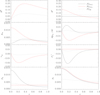 |
Fig. 1. Transversal equilibrium profiles of several quantities corresponding to models 𝒩ϕ77.5ℳ3.5β1, 𝒩ϕ45ℳ3.5β1, and ℱϕ77.5ℳ3.5β1, with the same averaged gas and magnetic pressures (ℳms, j = 3.5, βj = 1.0) and the three magnetic field configurations we considered. From left to right and from top to bottom: toroidal and axial magnetic fields, magnetic pressure relative to the mean magnetic pressure, magnetic pressure gradient, magnetic tension, radial component of the Lorentz force, gas pressure relative to the mean gas pressure, and total pressure relative to the mean total pressure. The filled and dotted black lines and filled red lines correspond to models 𝒩ϕ77.5ℳ3.5β1, 𝒩ϕ45ℳ3.5β1, and ℱϕ77.5ℳ3.5β1, respectively. The filled black lines coincide with the red filled lines in the panels with only two lines. |
Initial parameters defining our models.
3.2. Force-free magnetic field
For the force-free configuration, we kept the same profile for the toroidal magnetic field and changed the azimuthal profile, which is no longer homogeneous,
 (16)
(16)
It corresponds to the relativistic force-free diffuse pinch configuration defined in Lyutikov et al. (2005) (see Mizuno et al. 2015, and references therein for alternative force-free configurations). The maximum of Bz(r) (reached at the jet axis) is related to the maximum of the toroidal magnetic field,  , to cause the Lorentz force to become equal to zero, hence fixing the (mean) magnetic pitch angle ϕB, j (77.5°). Moreover, because the increase in the jet magnetization leaves the (constant) profile of the gas pressure unchanged in this case, the jet magnetization can grow without bound. We also note that the magnetic tension has the same expression as in the non-force-free models.
Figure 1 also displays one model (ℱϕ77.5ℳ3.5β1: see Table 1) corresponding to this case with the same mean gas and magnetic pressures as 𝒩ϕ45ℳ3.5β1 and 𝒩ϕ77.5ℳ3.5β1. The force-free character of model ℱϕ77.5 translates into a constant gas pressure profile (closer to the gas pressure profile of model 𝒩ϕ45ℳ3.5β1). On the other hand, because the magnetic tension profiles of models ℱϕ77.5ℳ3.5β1 and 𝒩ϕ77.5ℳ3.5β1 coincide, their total pressure profiles have the same local slopes. That these curves do not coincide (as they should, for models with the same total pressure) but are slightly different is the result of the construction of models with different magnetic field configurations for given average values and is a measure of the reliability of our comparison. This difference (of 7.0% in the averaged value of the total pressure between the two configurations) translates into two slightly different values of the parameter K1 (10%), which is the total pressure jump at the edge of the injection nozzle that governs the lateral expansion of the jet against the ambient medium (see next section).
4. Parameters defining the jet models
4.1. 𝒩ϕ45 models: Non-force-free configuration, ϕB,j = 45°
The jet models corresponding to this magnetic field configuration and pitch angle are a subset of those considered in Fuentes et al. (2018). The models are defined by specifying the values of ρj, pj, vj,  , and
, and  . However, this set of parameters is changed for practical reasons by the more meaningful set formed by the parameters ρj, vj, ℳms, j (the relativistic magnetosonic Mach number), βj (the jet magnetization), and ϕB, j, to which we added K, the jet overpressure factor (see Appendix A).
To reduce the dimensionality of the space of parameters, ρj, vj, K, and ϕB, j were fixed to 0.005ρa, 0.95c, 2, and 45°, respectively, in all the models. Table 1 lists the values of the remaining parameters defining them. The magnetosonic Mach number covers the range 2−10. The interval of the jet magnetization spans the full range of physical magnetizations, from almost zero (βj = 0.01) to the maximum allowed value that is compatible with a positive gas pressure at the jet surface (βj ≈ 17.5 for the current choice of jet parameters).
Quantity K1 in Table 1 is the jump in total pressure at the edge of the injection nozzle and controls the jet potential to expand against the ambient medium. As discussed in Sect. 5, a value of this quantity equal to K1, eq = 1 sets the equilibrium, whereas higher (lower) values cause the jet to expand (contract) in its effort to reach equilibrium. K1 would coincide with K, the average overpressure factor (equal to 2 in all the models considered), in the absence of magnetic tension and decreases as magnetic tension increases (in modulus) for constant internal and magnetic energies (see Eq. (19)). For a given configuration of the toroidal magnetic field and fixed magnetic pitch angle, the value of K1 is a decreasing function of the jet magnetization (Eq. (20)) in the absence of flow rotation. For the models listed in Table 1, K1 reaches a minimum value of ≈1.83 for the maximum magnetization (≈17.5), which is high enough to drive a significant lateral expansion of the jet against the ambient medium.
4.2. 𝒩ϕ77.5 models: Non-force-free configuration, ϕB,j = 77.5°
In this case, ρj, vj, and K were fixed to the same values as in the models of Sect. 4.1 (0.005ρa, 0.95c, and 2, respectively), whereas the magnetic pitch angle was now set to ϕB, j = 77.5°. The magnetosonic Mach number covered the same range (2−10) and the jet magnetization spanned the full physical range, from almost zero (βj = 0.01) to its maximum value (now as low as ≈2.34); see Table 1. Although the maximum attainable magnetization is now significantly lower than in models 𝒩ϕ45, the larger magnetic tension induced by the larger pitch angle of the helical magnetic field reduces the jump of total pressure at the jet surface to K1, min ≈ 1.16, which is close to the equilibrium value, K1, eq = 1. As a consequence, 𝒩ϕ77.5 models close to their maximum magnetization will prompt modest sideways expansions.
4.3. ℱϕ77.5 models: Force-free configuration
The parameters ρj, vj, and K and the interval of variation of ℳms, j were chosen as in the non-force-free case. The magnetic pitch angle (≈77.5°) was fixed by the force-free condition. In this case, the jet magnetization is unbounded, but we restricted it for practical purposes to the interval 0.01 to 100. In this range, K1 drops from a value of ≈2 to a value just below the equilibrium value, ≈0.98 (see Table 1). Models with magnetizations higher than ≈100 compress laterally to find the equilibrium beyond the injection point.
In a force-free plasma, the Lorentz force that is mutually exerted by the plasma and the magnetic field is zero everywhere. This can be the result of having a negligible gas pressure throughout the plasma or of specific equilibrium conditions fixed initially. Whereas in the first case, the force-free nature of the plasma tends to hold throughout the evolution of the plasma, force-free magnetic configurations specifically tuned as initial conditions can be destroyed (in the course of the evolution, or as the result of the growth of perturbations in a quasi-steady state) when the gas pressure is not negligible.
In our equilibrium configurations of magnetized jets, the jet magnetization βj measures the relative strength of the magnetic pressure with respect to the gas pressure. According to the previous paragraph, only force-free models with βj well above 1 are likely to survive as steady solutions and represent true steady force-free jet models. Finally, we note that in all our models, the force-free condition is broken at the jet surface where the jet is required to be in equilibrium with the ambient medium.
4.4. Models in the diagram of the magnetosonic Mach number and internal energy
Figure 2 displays models 𝒩ϕ45, 𝒩ϕ77.5, and ℱϕ77.5 in the diagram of the magnetosonic Mach number and internal energy. It is interesting to note that when the jet rest-mass density ρj and flow velocity vj are fixed, the models in the same point of the diagram of the Mach number and internal energy have the same gas pressure and magnetization (and consequently the same magnetic energy). The differences in the internal structure (shocks, transversal structure, lateral expansion, etc.) will therefore only depend on the magnetic field configuration (through the magnetic tension and the Lorentz force).
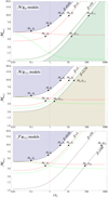 |
Fig. 2. Jet classes in the ℳms, j − 1/εj plane for different magnetic field configurations and magnetic pitch angles according to the dominant energy type for a given jet flow velocity, vj = 0.95c. The lines of constant magnetization are drawn. Kinetically dominated jets, magnetically dominated jets, and hot jets are placed in the diagram with the help of three (red) lines corresponding to models with c2 = εj, βj = 1, and βjεj = c2. Pure hydrodynamic models are placed on the βj = 0 line, which bounds a forbidden region (in violet) corresponding to unphysical models with negative magnetic energies. The distribution on the ℳms, j − 1/εj diagram of the models we considered is superimposed. |
On the other hand, it is interesting to note that the diagram of the magnetosonic Mach number and internal energy sorts the jet models into different regions of the diagram according to the dominant type of energy (internal, kinetic, or magnetic) or energy flux (internal, kinetic, or Poynting) in the jet. The red and green lines in the panels of Fig. 2 divide the regions where the different types of energy/energy fluxes dominate. Appendix A is devoted to defining these lines and the delimited regions.
The magnetization parameter σ (:=b2/ρh; see Table 1) of our models ranges from ∼10−3 for models with a passive magnetic field (β = 0.01) to almost 1 for the magnetically dominated jet models (those in the bottom right corner of Fig. 2; ℳ3.5 models with β > 1). Kinematically dominated jet models in the top half of Fig. 2 (cold high Mach-number jets; ℳ10 models with β ≥ 1) have σ ∼ 0.05−0.12. Finally, hot low Mach-number jets in equipartition (ℳ3.5 models with β = 1) have σ = 0.35.
4.5. Numerical method
Magnetohydrodynamical models were computed following the approach developed by Komissarov et al. (2015), which allowed us to study the structure of steady, axisymmetric, relativistic (magnetized) flows using one-dimensional time-dependent simulations. The approach is based on the fact that for narrow jets with axial velocities close to the light speed, the steady-state equations of relativistic magnetohydrodynamics can be accurately approximated by the one-dimensional time-dependent equations with the axial coordinate acting as the temporal coordinate.
The approximation is valid as long as the radial dimension of the flow is much smaller than the axial one, and simple quasi-one-dimensional flows are considered with the radial and azimuthal components of the flow velocity much lower than the axial component, which approaches light speed (i.e., vr, vϕ ≪ vz). Consistency with the one-dimensional version of the divergence-free condition forces us to consider configurations with very small radial components of the magnetic field (Br ≪ Bϕ, Bz). All these constraints can be verified a posteriori when the approximate two-dimensional solution has been obtained.
The more delicate point of the approximation consists of implementing the boundary conditions at the jet surface, which in the one-dimensional approximation become a kind of time-dependent boundary conditions. Special actions are required to mimic the effect of the two-dimensional steady boundary conditions at the jet surface: (i) The jet surface should be tracked throughout time, and (ii) the ambient gas parameters were reset at every computational time step according to the prescribed functions of time. Following Komissarov et al. (2015), the jet surface was tracked from the injection at the jet base using a passive scalar that was advected with the continuity equation. Second, in order to maintain the jet surface in a contact discontinuity, the radial velocity of the ambient gas was reset not to zero, but to its value at the last jet cell.
From a numerical point of view, the code that is used in these simulations is the one-dimensional radial-cylindrical time-dependent version of the RMHD code used in Martí (2015) and Martí et al. (2016). It is a second-order conservative finite-volume code based on high-resolution shock-capturing techniques. An overview of the specific algorithms used in the code and an analysis of its performance can be found in Appendices A and B, respectively, of Martí (2015). The code is the same as was used in Fuentes et al. (2018), where some specific tests were shown (an expanding jet with a purely azimuthal magnetic field into a pressure-decreasing atmosphere, and a comparison with steady truly two-dimensional models obtained by relaxation; see their Appendix A.2).
Numerical models were computed in a computational domain (r, z) ∈ [0, 4 Rj]×[0, 100 Rj] with 80 cells/Rj (radial) and 40 cells/Rj (axial) numerical resolution. We used a piecewise-linear reconstruction for the radial grid with the Van Leer-MinMod (VLMM) limiter and the Harten-Lax-Van Leer (HLL) Riemann solver. The integration along the axial coordinate was made using a third-order TVD-preserving Runge-Kutta with Courant-Friedrichs-Levy factor CFL = 0.4 (see Martí 2015, and references therein).
5. Lateral expansion in overpressured magnetized jets
Quantity K1 is defined as the total pressure jump at the edge of the injection nozzle. It determines the potential of the jet to expand against the ambient medium. A value of this quantity equal to K1, eq = 1 sets the equilibrium, whereas higher (lower) values cause the jet to expand (contract) in its effort to reach equilibrium. It would coincide with K, the average overpressure factor in the absence of magnetic tension, and would decrease as magnetic tension increases. This section is devoted to deriving simple expressions for the dependence of K1 on K and the average magnetic tension, and ultimately, on quantities such as the jet magnetization, the magnetic pitch angle, and the flow Lorentz factor, which are directly related with the parameters defining the jet.
As a starting point, we approximated the (average) total pressure, p*, and magnetic tension, τm, by the first-order expressions
 (17)
(17)
where R is the jet radius, and  and
and  stand for the total pressure at the axis and at the surface of the jet, respectively. These expressions are adequate in the absence of rotation because in this case, p*(r) is monotonic (Eq. (1)).
These equations can be solved for  to obtain
 (18)
(18)
Now, taking into account that K = p*/pa, and  (pa is the ambient pressure), we obtain the following expression relating the total pressure jump at the edge of the injection nozzle with the average total pressure jump
 (19)
(19)
We note that as τm < 0, K1 is always smaller than K, and it decreases when the magnetic tension increases (in absolute value) and increases (tends to K) when the total pressure increases.
The next step involves formulating τm/p* in terms of the parameters defining our jet models. First, we note that
where we have used the expression for the magnetic tension (Eq. (14)), the definition of the toroidal magnetic field (Eq. (12)), and the definition of the magnetic energy density (Eq. (A.3)). The proportionality constant only depends on Rm, the position of the maximum of Bϕ(r).
Finally, because b2/p* = β/(1 + β), the final expression reads
 (20)
(20)
where A is a (positive definite) function of Rm and R (which are fixed in all our models: Rm = 0.37 R, and R is the unit of length). The following conclusions are of interest:
-
K1 does not explicitly depend on the rest-mass density, internal energy, or any other thermodynamical variable defining the jet (although it does through β).
-
K1 increases with K and W. However, these two quantities have remained fixed for all our simulations.
-
For fixed ϕB, K1 decreases as β increases.
-
For fixed β, K1 decreases as ϕB increases.
6. Results for the magnetohydrodynamical jet structure, and discussion
For a fixed jet flow velocity and overpressure factor, the internal structure of nonmagnetized jets is determined exclusively by the relativistic Mach number (see, e.g., Martí et al. 2018, and references therein). Appendix B compares the internal structure of models with negligible magnetization and different magnetic field configurations and/or magnetic pitch angles, but with the same Mach number, as a reliability test of the numerical method we used. As a side result, the appendix reviews the internal structure (oblique shocks and radial oscillations) of purely hydrodynamical jets as a function of the Mach number.
6.1. 𝒩ϕ45 reference models
These models are a subset of those considered in Fuentes et al. (2018). In that work, we studied the resulting structure of the jets arising from the superposition of (i) the internal transversal equilibrium of the jet, and (ii) the recollimation shocks and sideways expansions and compressions of the jet flow induced by the total pressure mismatch at the interface of the jet and the ambient medium. The properties of recollimation shocks and radial oscillations were studied as functions of three scalar quantities defining the jet models, namely the magnetosonic (relativistic) Mach number, the specific internal energy in units of the specific rest-mass energy, and the magnetization. The selection of models considered in this paper, namely 𝒩ϕ45ℳ3.5β1, 𝒩ϕ45ℳ10β1, 𝒩ϕ45ℳ3.5β17.5, and 𝒩ϕ45ℳ10β17.5, which we use here as reference, appear in the top panels of Figs. 3, 5, 7, and 9, respectively. The jet radius and the averaged values of several quantities along the jet are shown in Figs. 4, 6, 8, and 10, and their relative variations along the jet are recorded in Table 2. The properties of shocks are reported in Table 3.
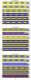 |
Fig. 3. Steady structure of models 𝒩ϕ45ℳ3.5β1, 𝒩ϕ77.5ℳ3.5β1, and ℱϕ77.5ℳ3.5β1 corresponding to relatively hot (εj = 1.72) low Mach-number (ℳms, j = 3.5) models in equipartition (βj = 1). From top to bottom: distributions of rest-mass density, gas pressure, toroidal flow velocity, flow Lorentz factor, and toroidal and axial magnetic field components. The poloidal flow and magnetic field lines are superposed onto the Lorentz factor and axial magnetic field panels, respectively. Two contour lines for the jet mass fraction values 0.05 and 0.95 are overplotted on the rest-mass density panel. |
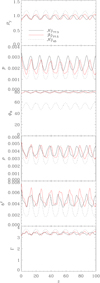 |
Fig. 4. Mean values along the jet for models 𝒩ϕ45ℳ3.5β1, 𝒩ϕ77.5ℳ3.5β1, and ℱϕ77.5ℳ3.5β1 corresponding to relatively hot (εj = 1.72) low Mach-number (ℳms, j = 3.5) models in equipartition (βj = 1). |
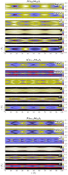 |
Fig. 5. Steady structure of models 𝒩ϕ45ℳ10β1, 𝒩ϕ77.5ℳ10β1, and ℱϕ77.5ℳ10β1 corresponding to to cold (εj = 0.09) high Mach-number (ℳms, j = 10) models in equipartition (βj = 1). Panel distribution as in Fig. 3. |
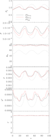 |
Fig. 6. Mean values along the jet for models 𝒩ϕ45ℳ10β1, 𝒩ϕ77.5ℳ10β1, an ℱϕ77.5ℳ10β1 corresponding to cold (εj = 0.09), high Mach-number (ℳms, j = 10) models in equipartition (βj = 1). |
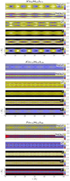 |
Fig. 7. Steady structure of magnetically dominated models 𝒩ϕ45ℳ3.5β17.5, 𝒩ϕ77.5ℳ3.5β2.34, and ℱϕ77.5ℳ3.5β100 corresponding to low Mach-number (ℳms, j = 3.5) models with magnetization β = 17.5, 2.34, and 100, respectively, and corresponding internal energies ε = 0.07, 0.57, and 0.01. Panel distribution as in Fig. 3. |
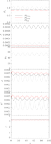 |
Fig. 8. Mean values along the jet for the magnetically dominated models 𝒩ϕ45ℳ3.5β17.5, 𝒩ϕ77.5ℳ3.5β2.34, and ℱϕ77.5ℳ3.5β100 corresponding to low Mach-number (ℳms, j = 3.5) models with magnetizations β = 17.5, 2.34, and 100, and corresponding internal energy ε = 0.07, 2.34, and 0.01. |
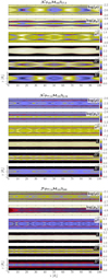 |
Fig. 9. Steady structure of kinetically dominated models 𝒩ϕ45ℳ10β17.5, 𝒩ϕ77.5ℳ10β2.34, and ℱϕ77.5ℳ10β100 corresponding to high Mach-number (ℳms, j = 10) models with the maximum magnetization (βmax = 17.5, 2.34, and 100, respectively) and correspondingly minimum internal energy (εmin = 0.01, 0.05, and 0.001). Panel distribution as in Fig. 3. |
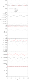 |
Fig. 10. Mean values along the jet for the kinetically dominated models 𝒩ϕ45ℳ10β17.5, 𝒩ϕ77.5ℳ10β2.34, and ℱϕ77.5ℳ10β100 corresponding to high Mach-number (ℳms, j = 10) models with magnetizations β = 17.5, 2.34, and 100, and corresponding internal energies ε = 0.01, 0.05, and 0.001. |
Relative variations along the jet of the quantities defining the steady models.
Properties of the recollimation shocks.
According to the results of Fuentes et al. (2018), for a fixed overpressure factor (and given magnetic field configuration and pitch angle), the strength of the recollimation shocks in superfast-magnetosonic jets increases for increasing internal energy density. This tendency holds for fixed Mach number (and decreasing magnetization) as well as for decreasing Mach number and constant magnetization. Finally, the strength of the recollimation shocks also tends to increase for fixed internal energy and decreasing magnetization (increasing Mach number). In summary, powerful recollimation shocks are found in hot jets with low Mach-number and low magnetization. In addition, the shock obliquity and the shock separation follow a remarkable correlation with the relativistic (magnetosonic) Mach number.
The properties of the radial oscillations follow those of the recollimation shocks. The change in the jet radius tends to increase with the Mach number for constant internal energy (decreasing magnetization). It also tends to increase with increasing internal energy for constant magnetic Mach number (decreasing magnetization) and constant magnetization (decreasing Mach number). The gas pressure follows the changes dictated by the adiabatic expansions/compressions of the flow (as a consequence of the variations in jet radius) plus the jumps at internal shocks. A similar behavior is found in the magnetic pressure, which is dominated by the axial component of the magnetic field. The changes in the Lorentz factor are larger in the hotter models (with more internal energy that can be exchanged into kinetic energy) and becomes negligible in cold kinetically dominated jets independently of the amplitude of the radial oscillations.
The results discussed in the previous paragraphs can be interpreted in light of Sect. 5, which relates the amplitude of radial oscillations with K1, the jump in total pressure at the edge of the injection nozzle. As discussed in that section, for this set of models, with the same magnetic pitch angle (and overpressure factor and flow Lorentz factor), K1 is a function of the magnetization βj only (Eq. (20)) and increases if βj decreases. On the other hand, the variations in thermodynamical variables and the Lorentz factor along the jet and the strength of the shocks is related to the amplitude of the radial oscillations, although they also depend on the amount of internal energy of the jet. We note in passing that the connection between jet opening angle (or amplitude of the jet radial oscillations) and the properties of internal shocks was recently studied by Monceau-Baroux et al. (2012). Finally, the action of the Lorentz force compels the internal energy to accumulate into a thin hot spine around the axis of highly magnetized jets.
6.2. Relativistic magnetized jets in equipartition
We now extend our analysis of the internal jet structure as a function of the magnetic field configuration and magnetic pitch angle to the case of magnetized jets in equipartition (βj = 1). The set of models {𝒩ϕ45ℳ3.5β1, 𝒩ϕ77.5ℳ3.5β1, and ℱϕ77.5ℳ3.5β1} corresponds to relatively hot (εj = 1.72) low Mach-number (ℳms, j = 3.5) jets, whereas the set {𝒩ϕ45ℳ10β1, 𝒩ϕ77.5ℳ10β1, and ℱϕ77.5ℳ10β1} corresponds to cold (εj = 0.09) high Mach-number (ℳms, j = 10) jets. It is interesting to recall (see Sect. 3) that for models at the same position in the diagram of the magnetosonic Mach number and internal energy, moving from the 𝒩ϕ45 model to the 𝒩ϕ77.5 model implies that magnetic tension and Lorentz force both increase, whereas moving from the 𝒩ϕ77.5 model to the ℱϕ77.5 model means that the Lorentz force drops to zero.
6.2.1. Hot jets with low Mach-number
Figure 3 displays three series of panels corresponding to models for hot jets with low Mach-number in equipartition, {𝒩ϕ45ℳ3.5β1, 𝒩ϕ77.5ℳ3.5β1, and ℱϕ77.5ℳ3.5β1}. Model 𝒩ϕ45ℳ3.5β1 corresponds to model M2B2 in Fuentes et al. (2018). From top to bottom, each series of panels shows two-dimensional distributions of proper rest-mass density, gas pressure (both in logarithmic scale), azimuthal flow velocity, flow Lorentz factor (with poloidal streamlines), and toroidal and axial magnetic field components. From a preliminary analysis of the figure we note that: (i) the sideways expansion of the jet is significantly larger in model 𝒩ϕ45ℳ3.5β1 than in models 𝒩ϕ77.5ℳ3.5β1 and ℱϕ77.5ℳ3.5β1, (ii) a prominent substructure is superimposed on the fundamental axial oscillation in models 𝒩ϕ77.5ℳ3.5β1 and ℱϕ77.5ℳ3.5β1, (iii) despite the overall similarity of models 𝒩ϕ77.5ℳ3.5β1 and ℱϕ77.5ℳ3.5β1, the gas pressure distributions are very different, with the gas pressure of model 𝒩ϕ77.5ℳ3.5β1 accumulating in a central spine around the axis, and (iv) the axial magnetic field is squeezed around the axis in model ℱϕ77.5ℳ3.5β1.
According to Sect. 5, points (i) and (ii) follow from the different magnetic tension of the models. As discussed in Sect. 4.1, the magnetic tension of model 𝒩ϕ45ℳ3.5β1 is weak enough to allow the jet to expand significantly. In contrast, the larger magnetic tension of models 𝒩ϕ77.5ℳ3.5β1 and ℱϕ77.5ℳ3.5β1 due to their larger magnetic pitch angle means that the sideways expansion of the flow is difficult, and it triggers a perturbation pattern of short wavelength inside the jet. The axially peaked distribution of the gas pressure in model 𝒩ϕ77.5ℳ3.5β1 (point (iii) above) is the result of the radial component of the Lorentz force, much larger than in models 𝒩ϕ45ℳ3.5β1 (due to the smaller pitch angle) and ℱϕ77.5ℳ3.5β1. Finally, the radial profile of the axial magnetic field (point (iv)) is a consequence of the force-free condition imposed on the magnetic field configuration of model ℱϕ77.5ℳ3.5β1.
Figure 4 shows the jet radius as well as the averaged values of rest-mass density, gas pressure, magnetic energy density, magnetic pitch angle, and flow Lorentz factor along the jet. The wider radial expansion of model 𝒩ϕ45ℳ3.5β1 (dotted black line in Fig. 4) leads to larger variations of gas and magnetic pressures, magnetic pitch angle, and Lorentz factor along the jet than in the other two models. The fundamental radial oscillation with remarkably the same axial wavelength is clearly seen in the three models, as is the substructure present in models 𝒩ϕ77.5ℳ3.5β1 and ℱϕ77.5ℳ3.5β1 (visible in the plots of the magnetic energy density and Lorentz factor). Table 2 gives a more quantitative account of these trends.
Table 3 shows the properties of the shocks following an analysis similar to that in Appendix B for purely hydrodynamical jets. However, the shock jumps in models 𝒩ϕ77.5ℳ3.5β1 and ℱϕ77.5ℳ3.5β1 are so small that only upper bounds of them can be provided. Despite the uncertainty of the estimate, these comfortably large upper bounds are enough to conclude that the strength of shocks is connected with the amplitude of the radial oscillations and that it decreases with the increase of the magnetic tension as expected from Sect. 5 (see Eq. (19)). The average gas pressure at the shocks,  , is higher in model 𝒩ϕ77.5ℳ3.5β1 because the Lorentz force pushes the gas pressure toward the axis. The average magnetic pressure,
  , is higher in model ℱϕ77.5ℳ3.5β1 because of the larger magnetic tension and the force-free magnetic field, which squeezes the axial magnetic field around the axis.
6.2.2. Cold jets with high Mach-number
We now concentrate on models for colder jets with higher Mach-number (i.e., kinetically dominated). Figure 5 displays three series of panels corresponding to cold (εj = 0.09) high Mach-number (ℳms, j = 10) models in equipartition, {𝒩ϕ45ℳ10β1, 𝒩ϕ77.5ℳ10β1, and ℱϕ77.5ℳ10β1}. Model 𝒩ϕ45ℳ10β1 corresponds to model M5B2 in Fuentes et al. (2018). The conclusions of the hot models discussed in Sect. 6.2.1 (wider sideways expansion of 𝒩ϕ45 model, prominent substructure in models 𝒩ϕ77.5 and ℱϕ77.5, axially peaked gas pressure distribution in model 𝒩ϕ77.5, and axial magnetic field squeezed around the axis in model ℱϕ77.5) are valid in this case as well and admit the same explanations based on the different magnetic tension and Lorentz force of the three models. Models {𝒩ϕ45ℳ10β1, 𝒩ϕ77.5ℳ10β1, and ℱϕ77.5ℳ10β1} have the same magnetization and magnetic pitch angle as their hot counterparts, models {𝒩ϕ45ℳ3.5β1, 𝒩ϕ77.5ℳ3.5β1, and ℱϕ77.5ℳ3.5β1}, and according to the discussion in Sect. 5, the amplitude of the radial oscillations must be approximately the same for the 𝒩ϕ45 (𝒩ϕ45ℳ10β1, 𝒩ϕ45ℳ3.5β1), 𝒩ϕ77.5 (𝒩ϕ77.5ℳ10β1, 𝒩ϕ77.5ℳ3.5β1), and ℱϕ77.5 (ℱϕ77.5ℳ10β1, ℱϕ77.5ℳ3.5β1) pairs. Differences in the wavelengths of the internal structure comes from the difference in Mach number between hot and cold models (Martí et al. 2016; Fuentes et al. 2018).
Figure 6 shows the jet radius and the averaged values of rest-mass density, gas pressure, magnetic energy density, magnetic pitch angle, and flow Lorentz factor along the jet and confirms the preliminary conclusions established in the previous paragraph. Table 2 compiles the relative variations of these quantities along the jet. The comparison with the data corresponding with the hot models in equipartition shows very similar relative variations of the jet radius (although with very different axial wavelengths) in models 𝒩ϕ45ℳ3.5β1 and 𝒩ϕ45ℳ10β1 on the one hand and with 𝒩ϕ77.5ℳ3.5β1, 𝒩ϕ77.5ℳ10β1, and ℱϕ77.5ℳ3.5β1, ℱϕ77.5ℳ10β1 on the other. As noted previously (Sects. 6.1 and 6.2.1), the relative variations of rest-mass density, gas pressure, magnetic energy density, magnetic pitch angle, and flow Lorentz factor are linked with the amplitude of the radial oscillations and are therefore larger for model 𝒩ϕ45ℳ10β1 than for models 𝒩ϕ77.5ℳ10β1 and ℱϕ77.5ℳ10β1. Additionally, the changes in the gas pressure and flow Lorentz factor are smaller in the cold models than in the hot ones. In particular, the change in Lorentz factor along the jet in the cold models is only 3%.
Table 3 shows the properties of the shocks in this set of models. As in the case of their hotter counterparts discussed in the previous section and according to the discussion in Sect. 5, the strength of shocks in this set decreases with the increase in magnetic tension (only conservative upper bounds for the jumps could be established for models 𝒩ϕ77.5ℳ10β1 and ℱϕ77.5ℳ10β1). The average gas and magnetic pressures across the shocks follow the same trends as in the hotter models (Sect. 6.2.1) with correspondingly lower values.
6.3. Relativistic highly magnetized jets
The next sets of models corresponds to jets with high magnetizations: βj = 100 in the case of the ℱϕ77.5 models and βj = βmax, with βmax the maximum magnetization attainable for models 𝒩ϕ45 (βmax = 17.5) and 𝒩ϕ77.5 (βmax = 2.34). The existence of a maximum magnetization in the non-force-free models arises from the fact that the Lorentz force tends to concentrate the gas pressure toward the jet axis at the expense of reducing it from the surface (see Sect. 3.1). Beyond some maximum magnetization, the Lorentz force is so large that there is no transversal equilibrium possible with a positive gas pressure at the interface of the jet and the ambient medium. In the case of force-free configurations, the connection between gas pressure profile and magnetization through the Lorentz force does not operate and the jet magnetization can grow without limit (see Sect. 3.2). We note that the models considered in this section are not at the same position in the diagram showing the magnetosonic Mach number and internal energy (see Fig. 2), and they are cold (εj < 1.0).
6.3.1. Magnetically dominated jets
The first set of models {𝒩ϕ45ℳ3.5β17.5, 𝒩ϕ77.5ℳ3.5β2.34, and ℱϕ77.5ℳ3.5β100} consists of magnetically dominated models with low Mach-number (ℳms, j = 3.5) with magnetizations βj = 17.5, 2.34, and 100 and correspondingly low internal energies εj = 0.07, 0.57, and 0.01. Model 𝒩ϕ45ℳ3.5β17.5 is the same as model M2B4 in Fuentes et al. (2018). As in the previous section, Fig. 7 displays three series of panels corresponding to these models. Although in this case the models under comparison are at different positions within the diagram of the magnetosonic Mach number and internal energy, the rough analysis of the three panels in Fig. 7 leads to similar conclusions as for the case of the equipartition models. Model 𝒩ϕ45ℳ3.5β17.5 undergoes the widest sideways expansion, whereas models 𝒩ϕ77.5ℳ3.5β2.34 and ℱϕ77.5ℳ3.5β100, which are much more alike, exhibit a prominent substructure. This is a consequence of the different magnetic tension, which is much lower in the case of model 𝒩ϕ45, and of the comparable total pressure of the three models, which according to Sect. 5 (Eq. (19)) leads to a higher value of K1 and hence to a larger amplitude of the radial oscillations. Finally, a noticeable difference with respect to the models in equipartition is that the axially peaked gas pressure profile is seen not only in model 𝒩ϕ77.5ℳ3.5β2.34, but also in 𝒩ϕ45ℳ3.5β17.5, as a result of the increase in the Lorentz force in this model with respect to the equipartition model.
The amplitude of the radial oscillations of models 𝒩ϕ45ℳ3.5β17.5, 𝒩ϕ77.5ℳ3.5β2.34, and ℱϕ77.5ℳ3.5β100 is easily spotted in Fig. 8, where we also show the mean values along the jet of some quantities characterizing the jet (gas pressure, magnetic pitch angle, rest-mass density, magnetic energy density, and flow Lorentz factor). Table 2 displays the relative variations of these quantities in the oscillations. The amplitude of the sideways expansion in models 𝒩ϕ77.5ℳ3.5β2.34 and ℱϕ77.5ℳ3.5β100 is so small that the magnetization, the magnetic pitch angle, and the flow Lorentz factor remain almost constant along the jet. The shocks in models 𝒩ϕ77.5ℳ3.5β2.34 and ℱϕ77.5ℳ3.5β100 are weaker than in model 𝒩ϕ45ℳ3.5β17.5 (see Table 3).
6.3.2. Kinetically dominated jets
The last set of models {𝒩ϕ45ℳ10β17.5, 𝒩ϕ77.5ℳ10β2.34, and ℱϕ77.5ℳ10β100} are kinetically dominated models with high Mach-number (ℳms, j = 10) with the same magnetizations β = 17.5, 2.34, and 100 as the previous set of models but correspondingly lower internal energies ε = 0.01, 0.05, and 0.001. Model 𝒩ϕ45ℳ10β17.5 corresponds to model M5B4 in Fuentes et al. (2018). The presentation of results is organized as for the previous cases. Figure 9 shows two-dimensional distributions of representative quantities, whereas the line plots with the variation of average values along the jet are shown in Fig. 10. Tables 2 and 3 compile the relative variations of several jet quantities along the radial oscillations and the jumps across shocks. As in the case of the hot and cold models in equipartition described in Sects. 6.2.1 and 6.2.2, respectively, the internal structure of the highly magnetized kinetically dominated jets presented in this section and the magnetically dominated jets of the previous section can be compared on the basis of their magnetic tension and Lorentz force. Models {𝒩ϕ45ℳ10β17.5, 𝒩ϕ77.5ℳ10β2.34, and ℱϕ77.5ℳ10β100} with the same magnetization and pitch angle as their magnetically dominated counterparts {𝒩ϕ45ℳ3.5β17.5, 𝒩ϕ77.5ℳ3.5β2.34, and ℱϕ77.5ℳ3.5β100} also have the same amplitude of the radial oscillations (as expected according to Sect. 5) and the same overall structure. The main differences between corresponding kinetically and magnetically dominated models is that the axial wavelength of the fundamental oscillation is larger in the kinetically dominated models, as anticipated for models with higher Mach number (Martí et al. 2016; Fuentes et al. 2018), and that the average pressure and magnetic field changes are correspondingly smaller in the kinetically dominated (i.e., colder) models. The axially peaked gas pressure profile is also seen in model 𝒩ϕ45ℳ10β17.5 as a result of the increase in the Lorentz force in this model with respect to the equipartition model. Again the internal structure of model 𝒩ϕ45ℳ10β17.5 is quite dissimilar to that of models 𝒩ϕ77.5ℳ10β2.34 and ℱϕ77.5ℳ10β100 (which are much more alike).
7. Summary and conclusions
The structure of axisymmetric, relativistic, superfast magnetosonic, overpressured jets was analyzed on the basis of the results for three sets of models with different magnetic pitch angles and helical magnetic field configurations (force-free and non-force-free). The present work extends the study of Fuentes et al. (2018) of the properties of recollimation shocks in connection with the dominant type of energy (internal, kinetic, or magnetic) in the jet to models with larger magnetic pitch angles and force-free magnetic fields.
Prior to these works, the properties of recollimation shocks in magnetized relativistic jets were studied by Mizuno et al. (2015) and more recently by Fromm et al. (2017). Mizuno et al. (2015) considered three models with axial, toroidal, and (force-free) helical magnetic fields. When projected onto the diagram of the magnetosonic (relativistic) Mach number and internal energy, the simulations of Mizuno et al. (2015) are placed on the line εj = 10.5 with magnetizations βj ∈ [0, 0.4]. The simulations of Fromm et al. (2017) correspond to models with εj ∼ 4.0 and magnetizations βj ∈ [0.54, 3.33]. Taken together, these simulations explore a tiny domain of the diagram of the Mach number and internal energy in the regions of hot jets that are mildly magnetized.
The magnetohydrodynamical models presented in this work were computed following the approach developed by Komissarov et al. (2015) for steady, axisymmetric, relativistic (magnetized) flows that was also used in Fuentes et al. (2018). The fundamental conclusions on the structure of jets established in Fuentes et al. (2018) for a narrower sample of non-force-free models with fixed magnetic pitch angle are confirmed, and we revealed the significance of the magnetic tension and the Lorentz force in shaping the internal structure of jets.
The internal structure of overpressured, superfast magnetosonic jets results from the superposition of (i) the internal transversal equilibrium of the jet and (ii) the recollimation shocks and sideways expansions and compressions of the jet flow.
-
(i)
The internal transversal equilibrium of the jet is controlled by the Lorentz force that permeates the jet. Under the action of the radial Lorentz force, the internal energy tends to accumulate into a thin hot spine around the axis of highly magnetized non-force-free jets at the expense of reducing it from the surface. Beyond some maximum magnetization, the Lorentz force is so large that no transversal equilibrium is possible with a positive gas pressure at the interface of the jet and the ambient medium. In the case of force-free configurations, the connection between gas pressure profile and magnetization through the Lorentz force does not operate, and the jet magnetization can grow without limit.
-
(ii.1)
The properties of the recollimation shocks and sideways expansions and compressions of the jet result from the total pressure mismatch at the edge of the injection nozzle, K1. In particular, K1 governs the amplitude of radial oscillations, ΔR. Higher values of K1 lead to larger amplitudes. Section 5 was devoted to deriving an approximate relation between K1 (and ΔR) and basic parameters defining the jet models. The results are listed below.
-
(ii.1.a)
As a function of the (mean) overpressure factor, K, the modulus of the (mean) magnetic tension across the jet, τm, and the total pressure (or internal plus magnetic energy density), p*: K1 (and ΔR) increases with K and p* and decreases with τm.
-
(ii.1.a)
As a function of the overpressure factor, K, the magnetic pitch angle, ϕB, the flow Lorentz factor, W, and the magnetization, β: K1 (and ΔR) increases with K and W and decreases with ϕB and β. As a result, models with large magnetic pitch angles and large magnetizations tend to have weaker shocks and radial oscillations of smaller amplitude than their counterparts with smaller magnetic pitch angle and magnetization.
-
(ii.1.a)
-
(ii.2)
The variations of the thermodynamical variables and the Lorentz factor along the jet and the strength of shocks (pressure jumps and jumps in Lorentz factor) are connected to the amplitude of the radial oscillations and hence to K1, although they also depend on the amount of internal energy that can be exchanged into kinetic energy in adiabatic expansions and compressions or at shocks. In particular, hot jets with low Mach-number have stronger shocks than cold jets with high Mach-number with the same magnetization and magnetic pitch angle.
-
(ii.3)
The wavelength of the oscillations along the jet and the shock separation and obliquity is governed by the (magnetosonic) Mach number. Low Mach-number jets tend to have tighter more oblique shocks than high Mach-number jets.
-
(ii.4)
In models with high magnetic tension, the magnetic pinch inhibits the sideways expansion of the flow. As a result, jets with large magnetic pitch angles have radial oscillations of small amplitude with a prominent internal substructure. The reduction of the amplitude of radial oscillations goes along with the decrease in the strength of internal shocks.
Our present study shows that magnetic tension (or the magnetic pitch angle) is the main parameter governing the equilibrium with the ambient medium, whereas the Lorentz force adjusts the transversal equilibrium inside the jet. In contrast, the role of the magnetization (defined here as the ratio of magnetic pressure to gas pressure) is less clear, and larger magnetic effects can be found in jets with moderate magnetization for configurations with larger Lorentz forces.
Our simulations are obviously limited by the imposed axisymmetry, which is not suitable to describe kink instabilities, and the time-independent condition, which does not allow the study of dynamical scenarios such as traveling components or the development of perturbations. In this respect, our simulations considering strong azimuthal magnetic fields can be highly dynamically unstable. Although the instabilities triggered by strong toroidal fields can be damped with a velocity shear and a current-sheet-free magnetic configuration (Kim et al. 2018), none of these conditions are fulfilled in our numerical setups. Nevertheless, this type of simulation allows us to obtain a better understanding of the physics that play a relevant role in conforming the transversal structure of the jets. In this respect, our simulations help understanding the origin of stationary structures in parsec-scale jets (see Fuentes et al. 2021) and inferring relevant intrinsic jet parameters. Furthermore, they can be used to establish initial equilibrium states for multidimensional dynamical simulations, as was done by Gourgouliatos & Komissarov (2018), for instance, in the case of non-magnetized relativistic hydrodynamics. It is our aim to follow the same strategy in the near future, with the aid of our new multidimensional fully parallelized RMHD code (López-Miralles et al., in prep.). The establishment of initial equilibria is relevant, for example, in multidimensional simulations studying the stability properties of jets (see, e.g., Perucho et al. 2004), or the evolution of perturbations propagating along parsec-scale jets (e.g., Agudo et al. 2001).
Acknowledgments
JMM and MP acknowledge financial support from the Spanish Ministerio de Economía y Competitividad (grant AYA2016-77237-C3-3-P), the Spanish Ministerio de Ciencia (PID2019-107427GB-C33), and from the local Autonomous Government (Generalitat Valenciana, grant PROMETEO/2019/071). JMM acknowledges further financial support from the Spanish Ministerio de Economía y Competitividad (grant PGC2018-095984-B-I00). MP acknowledges further financial support from the Spanish Ministerio de Ciencia through grant PID2019-105510GB-C31. AF and JLG acknowledge financial support from the Spanish Ministerio de Economía y Competitividad (grants AYA2016-80889-P, PID2019-108995GB-C21), the Consejería de Economía, Conocimiento, Empresas y Universidad of the Junta de Andalucía (grant P18-FR-1769), the Consejo Superior de Investigaciones Científicas (grant 2019AEP112), and the State Agency for Research of the Spanish MCIU through the Center of Excellence Severo Ochoa award for the Instituto de Astrofísica de Andalucía (SEV-2017-0709). This research made use of Python (http://www.python.org), Numpy (van der Walt et al. 2011), Pandas (McKinney 2010), and Matplotlib (Hunter 2007). We also made use of Astropy (http://www.astropy.org), a community-developed core Python package for Astronomy (Astropy Collaboration 2013, 2018).
References
- Agudo, I., Gómez, J.-L., Martí, J.-M., et al. 2001, ApJ, 549, L183 [NASA ADS] [CrossRef] [Google Scholar]
- Asada, K., Inoue, M., Uchida, Y., et al. 2002, PASJ, 54, L39 [NASA ADS] [Google Scholar]
- Astropy Collaboration (Robitaille, T. P., et al.) 2013, A&A, 558, A33 [NASA ADS] [CrossRef] [EDP Sciences] [Google Scholar]
- Astropy Collaboration (Price-Whelan, A. M., et al.) 2018, AJ, 156, 123 [Google Scholar]
- Begelman, M. C., Blandford, R. D., & Rees, M. J. 1984, Rev. Mod. Phys., 56, 255 [Google Scholar]
- Blandford, R. D., & Znajek, R. L. 1977, MNRAS, 179, 433 [Google Scholar]
- Casadio, C., Gómez, J. L., Grandi, P., et al. 2015a, ApJ, 808, 162 [Google Scholar]
- Casadio, C., Gómez, J. L., Jorstad, S. G., et al. 2015b, ApJ, 813, 51 [Google Scholar]
- Cohen, M. H., Meier, D. L., Arshakian, T. G., et al. 2014, ApJ, 787, 151 [NASA ADS] [CrossRef] [Google Scholar]
- Cohen, M. H., Meier, D. L., Arshakian, T. G., et al. 2015, ApJ, 803, 3 [NASA ADS] [CrossRef] [Google Scholar]
- Event Horizon Telescope Collaboration (Akiyama, K., et al.) 2019a, ApJ, 875, L1 [NASA ADS] [CrossRef] [Google Scholar]
- Event Horizon Telescope Collaboration (Akiyama, K., et al.) 2019b, ApJ, 875, L2 [NASA ADS] [CrossRef] [Google Scholar]
- Event Horizon Telescope Collaboration (Akiyama, K., et al.) 2019c, ApJ, 875, L3 [Google Scholar]
- Event Horizon Telescope Collaboration (Akiyama, K., et al.) 2019d, ApJ, 875, L4 [Google Scholar]
- Event Horizon Telescope Collaboration (Akiyama, K., et al.) 2019e, ApJ, 875, L5 [Google Scholar]
- Event Horizon Telescope Collaboration (Akiyama, K., et al.) 2019f, ApJ, 875, L6 [Google Scholar]
- Falle, S. A. E. G. 1991, MNRAS, 250, 581 [Google Scholar]
- Fromm, C., Porth, O., Younsi, Z., et al. 2017, Galaxies, 5, 73 [Google Scholar]
- Fuentes, A., Gómez, J. L., Martí, J. M., & Perucho, M. 2018, ApJ, 860, 121 [Google Scholar]
- Fuentes, A., Torregrosa, I., Martí, J. M., et al. 2021, A&A, 650, A61 (Paper II) [EDP Sciences] [Google Scholar]
- Gabuzda, D. 2018, Galaxies, 7, 5 [Google Scholar]
- Gabuzda, D. C., Roche, N., Kirwan, A., et al. 2017, MNRAS, 472, 1792 [Google Scholar]
- Gómez, J. L., Martí, J. M. A., Marscher, A. P., Ibáñez, J. M. A., & Marcaide, J. M. 1995, ApJ, 449, L19 [Google Scholar]
- Gómez, J. L., Martí, J. M., Marscher, A. P., Ibáñez, J. M., & Alberdi, A. 1997, ApJ, 482, L33 [NASA ADS] [CrossRef] [Google Scholar]
- Gómez, J. L., Marscher, A. P., Jorstad, S. G., Agudo, I., & Roca-Sogorb, M. 2008, ApJ, 681, L69 [Google Scholar]
- Gómez, J. L., Roca-Sogorb, M., Agudo, I., Marscher, A. P., & Jorstad, S. G. 2011, ApJ, 733, 11 [Google Scholar]
- Gómez, J. L., Lobanov, A. P., Bruni, G., et al. 2016, ApJ, 817, 96 [Google Scholar]
- Gourgouliatos, K. N., & Komissarov, S. S. 2018, Nat. Astron., 2, 167 [Google Scholar]
- Hovatta, T., Lister, M. L., Aller, M. F., et al. 2012, AJ, 144, 105 [Google Scholar]
- Hunter, J. D. 2007, Comput. Sci. Eng., 9, 90 [NASA ADS] [CrossRef] [Google Scholar]
- Jorstad, S. G., Marscher, A. P., Lister, M. L., et al. 2005, AJ, 130, 1418 [NASA ADS] [CrossRef] [Google Scholar]
- Jorstad, S. G., Marscher, A. P., Morozova, D. A., et al. 2017, ApJ, 846, 98 [NASA ADS] [CrossRef] [Google Scholar]
- Kim, J., Balsara, D. S., Lyutikov, M., & Komissarov, S. S. 2018, MNRAS, 474, 3954 [Google Scholar]
- Koide, S., Meier, D. L., Shibata, K., & Kudoh, T. 2000, ApJ, 536, 668 [Google Scholar]
- Komissarov, S. S. 1999, MNRAS, 308, 1069 [Google Scholar]
- Komissarov, S. S. 2001, MNRAS, 326, L41 [Google Scholar]
- Komissarov, S. S. 2004a, MNRAS, 350, 427 [Google Scholar]
- Komissarov, S. S. 2004b, MNRAS, 350, 1431 [Google Scholar]
- Komissarov, S. S. 2009, J. Korean Phys. Soc., 54, 2503 [Google Scholar]
- Komissarov, S. S. 2011, Mem. Soc. Astron. It., 82, 95 [NASA ADS] [Google Scholar]
- Komissarov, S. S., & Falle, S. A. E. G. 1997, MNRAS, 288, 833 [NASA ADS] [CrossRef] [Google Scholar]
- Komissarov, S. S., Barkov, M. V., Vlahakis, N., & Königl, A. 2007, MNRAS, 380, 51 [Google Scholar]
- Komissarov, S. S., Porth, O., & Lyutikov, M. 2015, Comput. Astrophys. Cosmol., 2, 9 [Google Scholar]
- Laing, R. A. 1981, ApJ, 248, 87 [Google Scholar]
- Lasota, J.-P., Gourgoulhon, E., Abramowicz, M., Tchekhovskoy, A., & Narayan, R. 2014, Phys. Rev. D, 89, 024041 [Google Scholar]
- Leismann, T., Antón, L., Aloy, M. A., et al. 2005, A&A, 436, 503 [NASA ADS] [CrossRef] [EDP Sciences] [Google Scholar]
- Lind, K. R., Payne, D. G., Meier, D. L., & Blandford, R. D. 1989, ApJ, 344, 89 [Google Scholar]
- Lister, M. L., Aller, M. F., Aller, H. D., et al. 2013, AJ, 146, 120 [Google Scholar]
- Lyutikov, M., Pariev, V. I., & Gabuzda, D. C. 2005, MNRAS, 360, 869 [Google Scholar]
- Marscher, A. P., Jorstad, S. G., D’Arcangelo, F. D., et al. 2008, Nature, 452, 966 [NASA ADS] [CrossRef] [PubMed] [Google Scholar]
- Marscher, A. P., Jorstad, S. G., Larionov, V. M., et al. 2010, ApJ, 710, L126 [NASA ADS] [CrossRef] [Google Scholar]
- Martí, J.-M. 2015, MNRAS, 452, 3106 [Google Scholar]
- Martí, J. M., Perucho, M., & Gómez, J. L. 2016, ApJ, 831, 163 [Google Scholar]
- Martí, J. M., Perucho, M., Gómez, J. L., & Fuentes, A. 2018, Int. J. Mod. Phys. D, 27, 1844011 [Google Scholar]
- McKinney, J. C. 2006, MNRAS, 368, 1561 [NASA ADS] [CrossRef] [Google Scholar]
- McKinney, W. 2010, in Proceedings of the 9th Python in Science Conference, eds. S. van der Walt, & J. Millman, 51 [Google Scholar]
- McKinney, J. C., & Blandford, R. D. 2009, MNRAS, 394, L126 [Google Scholar]
- McKinney, J. C., & Gammie, C. F. 2002, ApJ, 573, 728 [Google Scholar]
- McKinney, J. C., & Narayan, R. 2007, MNRAS, 375, 531 [Google Scholar]
- McKinney, J. C., Tchekhovskoy, A., & Blandford, R. D. 2012, MNRAS, 423, 3083 [Google Scholar]
- Mizuno, Y., Gómez, J. L., Nishikawa, K.-I., et al. 2015, ApJ, 809, 38 [NASA ADS] [CrossRef] [Google Scholar]
- Monceau-Baroux, R., Keppens, R., & Meliani, Z. 2012, A&A, 545, A62 [NASA ADS] [CrossRef] [EDP Sciences] [Google Scholar]
- Murphy, E., Cawthorne, T. V., & Gabuzda, D. C. 2013, MNRAS, 430, 1504 [Google Scholar]
- Penna, R. F., Narayan, R., & Sądowski, A. 2013, MNRAS, 436, 3741 [Google Scholar]
- Perucho, M., Martí, J. M., & Hanasz, M. 2004, A&A, 427, 431 [NASA ADS] [CrossRef] [EDP Sciences] [Google Scholar]
- Pushkarev, A. B., Gabuzda, D. C., Vetukhnovskaya, Y. N., & Yakimov, V. E. 2005, MNRAS, 356, 859 [Google Scholar]
- Tchekhovskoy, A., Narayan, R., & McKinney, J. C. 2011, MNRAS, 418, L79 [NASA ADS] [CrossRef] [Google Scholar]
- van der Walt, S., Colbert, S. C., & Varoquaux, G. 2011, Comput. Sci. Eng., 13, 22 [Google Scholar]
- Zamaninasab, M., Clausen-Brown, E., Savolainen, T., & Tchekhovskoy, A. 2014, Nature, 510, 126 [Google Scholar]
- Zavala, R. T., & Taylor, G. B. 2005, ApJ, 626, L73 [Google Scholar]
Appendix A: Diagram of the magnetosonic Mach number and internal energy for superfast magnetosonic relativistic jets
Relying on the conditions described in Sects. 2 and 3, we considered equilibrium models of relativistic, magnetized, axisymmetric, nonrotating jets propagating through a nonmagnetized ambient medium at rest. As explained in these sections, the jet solutions are characterized by five functions, namely the density and the pressure, ρj(r) and pj(r), respectively, the (axial) flow velocity,  , and the azimuthal and axial components of the magnetic field,
  and
and  . These functions are linked through the equation of transversal equilibrium, whereas a boundary condition at the jet surface sets the equilibrium with the ambient medium, characterized by a pressure, pa.
The jet models considered in this work were designed with uniform profiles for the rest-mass density and axial flow velocity, and some specific profiles for the magnetic field components. However, none of these choices is critical, and we can define the jet models by the corresponding average values of the rest-mass density and pressure, ρ and p, respectively, axial flow velocity, vz, and magnetic field components Bϕ and Bz, and the average jet overpressure factor, K, which is needed to fix the ambient pressure. Moreover, this set of parameters, namely {ρ, p, vz, Bϕ, Bz, and K}, is not unique, and some parameters can be suitably exchanged. For example, the gas pressure and the specific internal energy, ε, can be exchanged through the equation of state (and the rest-mass density). The exchange between the average components of the magnetic field and the magnetic pitch angle, ϕB, and the magnetization, β, is also interesting. The average magnetic pitch angle follows directly from
 (A.1)
(A.1)
The magnetization,
 (A.2)
(A.2)
follows from the gas pressure and the magnetic energy density, b2,
 (A.3)
(A.3)
where W is the average flow Lorentz factor.
Equations (A.1)–(A.3) (together with the equation of state) can be changed to define the models through the set of parameters {ρ, ε, vz, ϕB, β, and K}.
The remaining parameters characterizing the jet model can be derived from these sets of parameters. For example, the relativistic magnetosonic Mach number, governing the properties of the internal conical shocks in overpressured magnetized jets, follows from its definition (Cohen et al. 2015; Martí et al. 2016)
 (A.4)
(A.4)
taking into account that Wms is the Lorentz factor associated with the magnetosonic speed (an upper limit of the fast magnetosonic wave speed), cms,
 (A.5)
(A.5)
which in turn is defined in terms of the sound speed, cs, and the Alfvén speed, cA,
 (A.6)
(A.6)
In the previous expressions, the sound speed, cs, and the specific enthalpy, h, are known in terms of the rest-mass density and pressure (or specific internal energy) through the equation of state.
Models with the same rest-mass density, axial flow velocity, magnetic pitch angle, overpressure factor, and varying specific internal energy and magnetization can be sorted into a diagram of the magnetosonic Mach number and specific internal energy such as the one shown in Fig. A.1, corresponding to the models described in Sect. 4.1. The black lines in this diagram represent the internal energies and magnetosonic Mach numbers of models with some specified magnetization. The upper line corresponds to purely hydrodynamical models (i.e., β = 0), whereas the lower line shows models with the maximum magnetization compatible with a positive gas pressure at the jet surface. Physical models with positive magnetic energies and positive gas pressures are only found in the white region of the diagram between these two lines.
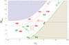 |
Fig. A.1. ℳms, j − 1/εj plane for magnetic field configuration 1 and magnetic pitch angle 45° defining the regions in which jets are dominated by kinetic, internal, or magnetic energies (separated by red lines), and kinetic, internal, or Poynting fluxes (separated by the vertical red line and the green lines). See text for the region labeling. |
Another interesting feature of the diagram of the magnetosonic Mach number and internal energy is that it sorts the jet models into different regions of the diagram according to the dominant type of energy (internal, kinetic, or magnetic) or energy flux (internal, kinetic, or Poynting) in the jet. The red and green lines depicted in Fig. A.1 divide the regions in which the different types of energy and energy fluxes dominate.
We first consider the red lines. The vertical red line εj = c2 separates models in which internal energy dominates the kinetic energy (placed at the left of the line) from those in which the opposite occurs. The red line in the white region between the βj = 1 and βj = βmax is the line βj = 1 and separates the models in which internal energy dominates the magnetic one (above the line) from those in which the opposite occurs. The remaining line, βjεj = c2, separates models in which kinetic energy dominates the magnetic one (above the line) from those in which the opposite occurs. To summarize, the diagram of magnetosonic Mach number and internal energy can be divided into six regions according to the dominant energy densities of their jet models:
-
Region KH: εj < c2, βj < 1.
-
Region KM: βj > 1, βjεj < c2.
-
Region MK: βjεj > c2, εj < c2.
-
Region MH: εj > c2, βj > 1.
-
Region HM: βj < 1, βjεj > c2.
-
Region HK: βjεj < c2, εj > c2.
In this list, K, H, and M stand for kinetic, internal, and magnetic energies, respectively, and their ordering in the names of the regions reflects their relative weight in defining the total energy density of the jet at injection.
The previous analysis can be extended to the dominant energy flux considering again the vertical red line and the two green lines. The red line is now used to separate models in which the internal energy flux dominates the kinetic energy flux (Fi > Fk; at the left of the line) from those in which the opposite occurs. The green line in the white region separates models in which the internal energy flux dominates the Poynting flux (Fi > FP; above the line) from those in which the opposite occurs. It corresponds to β = βP, where βP in the minimum magnetization needed for a jet with nonzero poloidal field to be dominated by Poynting flux,
 (A.7)
(A.7)
The last line βjεj = βPc2, separates models in which the kinetic energy flux dominates the Poynting flux (above the line) from those in which the opposite occurs:
-
Region KH: εj < c2, βj < βP.
-
Region KP: βj > βP, βjεj < βPc2.
-
Region PK: βjεj > βPc2, εj < c2.
-
Region PH: εj > c2, βj > βP.
-
Region HP: βj < βP, βjεj > βPc2.
-
Region HK: βjεj < βPc2, εj > c2.
K, H, and P stand for kinetic, internal, and Poynting fluxes, respectively, and their ordering in the names of the regions reflects their relative weight in defining the total energy flux of the jet at injection.
Appendix B: Relativistic jets with a passive magnetic field
Jets with βj = 0.01 can be understood as purely hydrodynamical models with a passive magnetic field. In this case, for a fixed jet flow velocity and overpressure factor, the internal structure of the jets is exclusively determined by the relativistic Mach number (see, e.g., Martí et al. 2018, and references therein) independently of the configuration of the magnetic field. The sets of models {𝒩ϕ45ℳ4.5β0, 𝒩ϕ77.5ℳ4.5β0, and ℱϕ77.5ℳ4.5β0}, {𝒩ϕ45ℳ6β0, 𝒩ϕ77.5ℳ6β0, and ℱϕ77.5ℳ6β0} and {𝒩ϕ45ℳ10β0, 𝒩ϕ77.5ℳ10β0, and ℱϕ77.5ℳ10β0}, corresponding to different magnetic field configurations and/or magnetic pitch angles, but with the same Mach number (4.5, 6, and 10, respectively; see the position of the models in the diagrams of Fig. 2) have an almost indistinguishable hydrodynamical structure (rest-mass density, gas pressure, and flow velocity). As a sample, model 𝒩ϕ77.5ℳ4.5β0, shown in Fig. B.1, can be compared with model M3B1 (𝒩ϕ45) appearing in Fig. 3 of Fuentes et al. (2018). The differences arise in the azimuthal flow velocity (which must be negligible compared with the axial component, i.e., much lower than 1 in light speed units) and the magnetic field, which has a different pitch angle in the two models. However, the maxima and minima of rest-mass density, pressure, and axial flow Lorentz factor are almost identical, as is their overall structure, including the position of shocks and the amplitude of the radial oscillations (we note the different radial to axial scales used in the two figures, 1:1 in Fig. 3 of Fuentes et al. 2018, 1.5:1 in Fig. B.1).
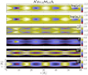 |
Fig. B.1. Steady structure of the hot jet model 𝒩ϕ77.5ℳ4.5β0 with the non-force-free magnetic field configuration and magnetic pitch angle 45°. From top to bottom: distributions of rest-mass density, gas pressure, toroidal flow velocity, flow Lorentz factor, and toroidal and axial magnetic field components. Poloidal flow and magnetic field lines are superimposed onto the Lorentz factor and axial magnetic field panels, respectively. Two contour lines for jet mass fraction values 0.05 and 0.95 are overplotted on the rest-mass density panel. |
We now concentrate on the internal structure of these nonmagnetized jets as a function of Mach number (or equivalently, as a function of internal energy density). Tables B.1 and B.2 compile the properties of internal shocks and average variations along the jet for models 𝒩ϕ45ℳ4.5β0, 𝒩ϕ45ℳ6β0, and 𝒩ϕ45ℳ10β0, which we take as reference for nonmagnetized models. These models correspond to models M3B1, M4B1, and M5B1, respectively, of Fuentes et al. (2018) but were not discussed separately.
Nonmagnetized models: properties of the recollimation shocks.
Nonmagnetized models: relative variations along the jet of the quantities defining the steady models.
The properties of the shocks are characterized in the same way as in Fuentes et al. (2018). The energy involved in the shocks can be estimated through the average of gas pressure across the shock,  . In this expression, subindex 1 (2) refers to pre-(post-)shock quantities. A criterion for determining the shock strength is the magnitude of the jumps of gas pressure, Δps = p2/p1. Finally, the jump in the flow Lorentz factor is connected to the jump in gas pressure. Quantities ΔΓ = Γ1/Γ2 (we note the change in the definition with respect to Δps) and
  define the jump in Lorentz factor and the average between the pre- and post-shock values, respectively.
The jumps presented in Table B.1 were calculated at a particular radius close to the jet axis where the shocks can be more planar and hence stronger than at larger radii. The high values of the gas pressure jumps (in the range ≈20−30) indicate that the shocks are strong close to the axis (however, the small deviation of the shock sequence from periodicity implies that the shocks are weak overall). From the data shown in the table, we conclude that the jumps of gas pressure and flow Lorentz factor decrease for decreasing εj (i.e., increasing relativistic Mach numbers). As discussed in Martí et al. (2016) and Fuentes et al. (2018), these trends are consistent with the fact that the strength of the shocks depends on the internal energy of the jet, which establishes the amount of energy that can be exchanged into kinetic energy at shocks. The shock obliquity (as determined by ϕs, the angle between the shock and the jet axis; see the last column in Table B.1) and the shock separation (which coincides with the axial wavelength of the radial oscillations listed in the last column of Table B.2) follows a remarkable correlation with the relativistic Mach number (which controls the angle at which waves penetrate the jet, or Mach angle, whose steepening forms the recollimation shocks). Finally, there is also a correlation between the average gas pressure involved at the shocks and the ambient pressure, the former being up to 80% of the latter. For purely hydrodynamic jets, this was noted before by Falle (1991).
Together with the sequence of recollimation shocks, the jets exhibit a series of radial oscillations with the same periodicity. Table B.2 lists the relative average variation of several relevant jet quantities along the jet as a result of the radial expansions and compressions. For these nonmagnetized models, K1 is approximately constant to its possible maximum value (K = 2). Hence, according to the discussion in Sect. 5, we would expect radial oscillations with the largest amplitudes and almost independent of the model considered. The results show that the jet radii change by ≈40−50%, with a slight tendency of the oscillation amplitude to increase with the Mach number (i.e., to decrease with internal energy density). The pressure changes by the adiabatic expansions and compressions of the flow along the jet and the jumps at internal shocks, and displays variations of a few (≈3) units. The changes in the Lorentz factor reflect the potential of the jet flow to exchange internal and kinetic energies and are larger in the hotter models and become negligible in cold, kinetically dominated jets in spite of the large radial oscillations. The last column in Table B.2 records the axial wavelength of the oscillations in the different models.
All Tables
Nonmagnetized models: relative variations along the jet of the quantities defining the steady models.
All Figures
|
Fig. 1. Transversal equilibrium profiles of several quantities corresponding to models 𝒩ϕ77.5ℳ3.5β1, 𝒩ϕ45ℳ3.5β1, and ℱϕ77.5ℳ3.5β1, with the same averaged gas and magnetic pressures (ℳms, j = 3.5, βj = 1.0) and the three magnetic field configurations we considered. From left to right and from top to bottom: toroidal and axial magnetic fields, magnetic pressure relative to the mean magnetic pressure, magnetic pressure gradient, magnetic tension, radial component of the Lorentz force, gas pressure relative to the mean gas pressure, and total pressure relative to the mean total pressure. The filled and dotted black lines and filled red lines correspond to models 𝒩ϕ77.5ℳ3.5β1, 𝒩ϕ45ℳ3.5β1, and ℱϕ77.5ℳ3.5β1, respectively. The filled black lines coincide with the red filled lines in the panels with only two lines. |
| In the text | |
|
Fig. 2. Jet classes in the ℳms, j − 1/εj plane for different magnetic field configurations and magnetic pitch angles according to the dominant energy type for a given jet flow velocity, vj = 0.95c. The lines of constant magnetization are drawn. Kinetically dominated jets, magnetically dominated jets, and hot jets are placed in the diagram with the help of three (red) lines corresponding to models with c2 = εj, βj = 1, and βjεj = c2. Pure hydrodynamic models are placed on the βj = 0 line, which bounds a forbidden region (in violet) corresponding to unphysical models with negative magnetic energies. The distribution on the ℳms, j − 1/εj diagram of the models we considered is superimposed. |
| In the text | |
|
Fig. 3. Steady structure of models 𝒩ϕ45ℳ3.5β1, 𝒩ϕ77.5ℳ3.5β1, and ℱϕ77.5ℳ3.5β1 corresponding to relatively hot (εj = 1.72) low Mach-number (ℳms, j = 3.5) models in equipartition (βj = 1). From top to bottom: distributions of rest-mass density, gas pressure, toroidal flow velocity, flow Lorentz factor, and toroidal and axial magnetic field components. The poloidal flow and magnetic field lines are superposed onto the Lorentz factor and axial magnetic field panels, respectively. Two contour lines for the jet mass fraction values 0.05 and 0.95 are overplotted on the rest-mass density panel. |
| In the text | |
|
Fig. 4. Mean values along the jet for models 𝒩ϕ45ℳ3.5β1, 𝒩ϕ77.5ℳ3.5β1, and ℱϕ77.5ℳ3.5β1 corresponding to relatively hot (εj = 1.72) low Mach-number (ℳms, j = 3.5) models in equipartition (βj = 1). |
| In the text | |
|
Fig. 5. Steady structure of models 𝒩ϕ45ℳ10β1, 𝒩ϕ77.5ℳ10β1, and ℱϕ77.5ℳ10β1 corresponding to to cold (εj = 0.09) high Mach-number (ℳms, j = 10) models in equipartition (βj = 1). Panel distribution as in Fig. 3. |
| In the text | |
|
Fig. 6. Mean values along the jet for models 𝒩ϕ45ℳ10β1, 𝒩ϕ77.5ℳ10β1, an ℱϕ77.5ℳ10β1 corresponding to cold (εj = 0.09), high Mach-number (ℳms, j = 10) models in equipartition (βj = 1). |
| In the text | |
|
Fig. 7. Steady structure of magnetically dominated models 𝒩ϕ45ℳ3.5β17.5, 𝒩ϕ77.5ℳ3.5β2.34, and ℱϕ77.5ℳ3.5β100 corresponding to low Mach-number (ℳms, j = 3.5) models with magnetization β = 17.5, 2.34, and 100, respectively, and corresponding internal energies ε = 0.07, 0.57, and 0.01. Panel distribution as in Fig. 3. |
| In the text | |
|
Fig. 8. Mean values along the jet for the magnetically dominated models 𝒩ϕ45ℳ3.5β17.5, 𝒩ϕ77.5ℳ3.5β2.34, and ℱϕ77.5ℳ3.5β100 corresponding to low Mach-number (ℳms, j = 3.5) models with magnetizations β = 17.5, 2.34, and 100, and corresponding internal energy ε = 0.07, 2.34, and 0.01. |
| In the text | |
|
Fig. 9. Steady structure of kinetically dominated models 𝒩ϕ45ℳ10β17.5, 𝒩ϕ77.5ℳ10β2.34, and ℱϕ77.5ℳ10β100 corresponding to high Mach-number (ℳms, j = 10) models with the maximum magnetization (βmax = 17.5, 2.34, and 100, respectively) and correspondingly minimum internal energy (εmin = 0.01, 0.05, and 0.001). Panel distribution as in Fig. 3. |
| In the text | |
|
Fig. 10. Mean values along the jet for the kinetically dominated models 𝒩ϕ45ℳ10β17.5, 𝒩ϕ77.5ℳ10β2.34, and ℱϕ77.5ℳ10β100 corresponding to high Mach-number (ℳms, j = 10) models with magnetizations β = 17.5, 2.34, and 100, and corresponding internal energies ε = 0.01, 0.05, and 0.001. |
| In the text | |
|
Fig. A.1. ℳms, j − 1/εj plane for magnetic field configuration 1 and magnetic pitch angle 45° defining the regions in which jets are dominated by kinetic, internal, or magnetic energies (separated by red lines), and kinetic, internal, or Poynting fluxes (separated by the vertical red line and the green lines). See text for the region labeling. |
| In the text | |
|
Fig. B.1. Steady structure of the hot jet model 𝒩ϕ77.5ℳ4.5β0 with the non-force-free magnetic field configuration and magnetic pitch angle 45°. From top to bottom: distributions of rest-mass density, gas pressure, toroidal flow velocity, flow Lorentz factor, and toroidal and axial magnetic field components. Poloidal flow and magnetic field lines are superimposed onto the Lorentz factor and axial magnetic field panels, respectively. Two contour lines for jet mass fraction values 0.05 and 0.95 are overplotted on the rest-mass density panel. |
| In the text | |
Current usage metrics show cumulative count of Article Views (full-text article views including HTML views, PDF and ePub downloads, according to the available data) and Abstracts Views on Vision4Press platform.
Data correspond to usage on the plateform after 2015. The current usage metrics is available 48-96 hours after online publication and is updated daily on week days.
Initial download of the metrics may take a while.