© X. Chen et al. 2021

1. Introduction

Radiative transfer for photons passing through a plasma (i.e., photon-electron scattering) is an important topic in both astrophysics and radiation physics. The transfer process, known as Comptonization, significantly affects the properties of emergent radiation from plasmas, for example the spectral shape of the continuum, the profile and centroid energy of an emission or absorption line, the intensity ratio of different lines, and the polarization (Fabian et al. 1995; Misra & Kembhavi 1998; Titarchuk 1994). The detailed consideration of the problem of energy transfer between the radiation and the medium is as important as that of the basic radiation mechanism, particularly in the X-ray band. With the rapid development of X-ray astronomy in recent years, it seems necessary to have an effective theory that describes the radiative transfer process (Kompaneets 1957; Illarionov et al. 1979; Fabian et al. 1995; Sunyaev & Titarchuk 1985; Titarchuk 1994; Hua et al. 1997; Kazanas et al. 1997; Misra & Kembhavi 1998; Zhang et al. 2000; Liu et al. 2004; Felten & Rees 1972; Miyamoto 1978). When high-energy photons go through the media surrounding them, these media may be ionized into plasma. We note the specialty of the radiative transfer in X-ray band: for an almost fully ionized plasma at high temperature, which often occurs in high-energy astrophysics, the dominant mechanism of energy exchange between radiation and plasma is nonelastic photon-electron scattering. This special transfer mechanism in X-ray astronomy is known as Comptonization. Comptonization is also of vital importance in astro-particle physics.

Although the change of the photon wavelength (or energy) in each individual collision between a photon and an electron is very small, the integrated variation in photon energy in multiple Compton scatterings in actual astronomical circumstances may be significant, particularly for the hard X-ray and γ-ray photons. The fractional change of the photon wavelength or frequency in each collision is given by the well-known formula (if the electron is approximately motionless before collision)

$$\begin{array}{c}\hfill \frac{\mathrm{\Delta }\lambda }{\lambda }=\frac{{\lambda }^{\prime }-{\lambda }_0}{{\lambda }_0}=\frac{2{\lambda }_{\mathrm{C}}}{{\lambda }_0}{sin}^2\frac{\theta }{2}\approx \frac{{\lambda }_{\mathrm{C}}}{{\lambda }_0},\end{array}$$(1)

where λ_C ≡ h/m_ec = 0.024 Å is the Compton wavelength and θ is the scattering angle. It is seen from Eq. (1) that the fractional change $\frac{\mathrm{\Delta }\lambda }{{\lambda }_0}$ depends on the initial wavelength λ₀. The shorter the initial wavelength λ₀ is, the larger the change $\frac{\mathrm{\Delta }\lambda }{{\lambda }_0}$ will be. For example, $\frac{\mathrm{\Delta }\lambda }{{\lambda }_0}\approx {10}^{-6}$ for λ₀ = 5000 Å in the optical band, but $\frac{\mathrm{\Delta }\lambda }{{\lambda }_0}\approx {10}^{-2}$ if λ₀ ≃ 0.5 Å (hν ∼ 20 keV, in the X-ray band). For a very hard γ-ray photon with energy ∼100 keV, $\frac{\mathrm{\Delta }\lambda }{{\lambda }_0}\approx {10}^{-1}$. This is why Comptonization is particularly important in hard X-ray and γ-ray astronomy.

Generally, we use the Kompaneets equation to describe Comptonization,

$$\begin{array}{c}\hfill {\left(\frac{\partial n}{\partial t}\right)}_c=\frac{k{T}_{\mathrm{e}}}{m_{\mathrm{e}}{c}^2}{N}_{\mathrm{e}}{\sigma }_{\mathrm{T}}c\frac{1}{x^2}\frac{\partial }{\partial x}\left\{x^4[\frac{\partial n}{\partial x}+n(n+1)]\right\},\end{array}$$(2)

where x ≡ hν/kT_e is the dimensionless photon energy; kT_e is the electron temperature; N_e is the number density of the scattering electron gas; σ_T is the Thomson cross section; and n(x, t) ≡ n(ν, t) is the frequency distribution function of the photon gas. The Kompaneets equation describes the Comptonization scattering of low-energy photons of frequency ν on a dilute distribution of nonrelativistic electrons when all photons and electrons are distributed isotropically in their momenta. The Kompaneets equation is applicable when the photon energy hν ≪ kT_e ≪ m_ec². However, it fails in describing the Comptonization of high-energy photons passing through electron plasma, which is the most important radiative transfer process in hard X-ray and γ-ray astronomy.

Based on the Fokker-Plank equation, Ross et al. (1978) obtained the Ross–McCray equation to describe Compton scattering:

$$\begin{array}{c}\hfill {\left(\frac{\partial n}{\partial t}\right)}_c=\frac{k{T}_{\mathrm{e}}}{m_{\mathrm{e}}{c}^2}{N}_{\mathrm{e}}{\sigma }_{\mathrm{T}}c\frac{1}{x^2}\frac{\partial }{\partial x}\left\{x^4[n+(1+\frac{7}{10}\frac{k{T}_{\mathrm{e}}}{m_{\mathrm{e}}{c}^2}{x}^2)\frac{\partial n}{\partial x}]\right\}·\end{array}$$(3)

Strictly, for the diffusion equation, when the photon gas reaches a thermal equilibrium with the electrons, $\frac{\partial n}{\partial t}=0$ should be satisfied. While inserting the Planck distribution function n(x) = (e^x − 1)⁻¹ into Eq. (3), $\frac{\partial n}{\partial t}\ne 0$. This means that the Ross–McCray equation does not conserve the number of photons.

Liu et al. (2004) extended the Kompaneets equation, with the goal of describing a more general Compton scattering process:

$$\begin{array}{cc}\hfill {\left(\frac{\partial n}{\partial t}\right)}_c=& \frac{k{T}_{\mathrm{e}}}{m_{\mathrm{e}}{c}^2}{N}_{\mathrm{e}}{\sigma }_{\mathrm{T}}c\frac{1}{x^2}\hfill \\ \hfill & \times \frac{\partial }{\partial x}\left\{x^4(1+\frac{7}{10}\frac{k{T}_{\mathrm{e}}}{m_{\mathrm{e}}{c}^2}{x}^2)[\frac{\partial n}{\partial x}+n(n+1)]\right\}·\hfill \end{array}$$(4)

Kompaneets & Eksper (1956), Kompaneets (1957) assumed that Δν is also a small quantity when hν ≫ kT_e. Then he used Δν to expand the distribution function, but this condition is not always satisfied. The change in photon energy is (Kompaneets 1957)

$$\begin{array}{c}\hfill h\mathrm{\Delta }\nu =-\frac{h\nu c\mathit{p}·(\mathit{n}-{\mathit{n}}^{\prime })+{(h\nu )}^2(1-\mathit{n}·{\mathit{n}}^{\prime })}{m_{\mathrm{e}}{c}^2[1+(h\nu /m_{\mathrm{e}}{c}^2)(1-\mathit{n}·{\mathit{n}}^{\prime })-\mathit{p}·{\mathit{n}}^{\prime }/\left(m_{\mathrm{e}}c\right)]}·\end{array}$$(5)

The momentum of thermal electrons is $p\sim m_{\mathrm{e}}\mathit{v}\sim m_{\mathrm{e}}\sqrt{k{T}_{\mathrm{e}}/m_{\mathrm{e}}}$. So in Eq. (4) the ratio of the second term in the numerator to the first term is $\sqrt{(h\nu /m_{\mathrm{e}}{c}^2)(h\nu /k{T}_{\mathrm{e}})}$. When hν is large enough, as Liu et al. (2004) argued, the second term in the numerator cannot be neglected. Hence in this paper we keep the second term. It is the first difference between our derivation and Kompaneets’. The second difference is that we re-derive the Kompaneets equation by expanding the distribution function with respect to the change in the electron’s momentum Δp. We see that Δp expansion is more reasonable than Δν in both cases: hν ≫ kT_e and hν ≪ kT_e.

This paper is organized as follows. In Sect. 2 we follow the Kompaneets method to improve the derivation of the diffuse equation for describing the Comptonization process of photon gas, and obtain a new modified form of the Kompaneets equation in a novel way. Then in Sect. 3 we compare our new equation with the Kompaneets equation by calculating the spectral evolution behavior of the Gaussian emission lines. In Sect. 4, based on the newly obtained equation and the Kompaneets equation, the evolution behavior of the blackbody spectra are displayed under some typical circumstances for high-energy astrophysics, and the Sunyaev-Zel’dovich effect is also investigated by involving our new equation. Finally, our conclusions and discussions are given in Sect. 5, in which the potential applications of the extended equation in astrophysics are highly emphasized. Additional Comptonization figures of the spectrum under various conditions can be found in Appendix A.

2. New approach to modify the Kompaneets equation

According to the Kompaneets method (Kompaneets & Eksper 1956; Kompaneets 1957), we treat the radiation as a closed system that consists of a photon gas and an electron gas. Although the system cannot be described by a characteristic temperature before the thermal equilibrium is established, the electron gas itself is already in thermal equilibrium as the interaction between electrons is the Coulomb long-range force. For the tenuous plasma, the Fermi distribution of electron gas approximately equals the Boltzmann distribution:

$$\begin{array}{c}\hfill f(p)=f_{0}exp[-\frac{1}{k{T}_{\mathrm{e}}}\frac{p^2}{2m_{\mathrm{e}}}]·\end{array}$$(6)

Because the photon is a boson, it does not affect the electron gas distribution, but it is capable of absorption and radiation of energy of all frequencies. Over a sufficiently long time, the absorption and emission of the photon gas caused by the scattering of electrons and photons will lead to thermal equilibrium.

In the electron and photon collision process such that (p, ν, n)→(p′, ν′,n′), there will be a decrease in the photon number n(ν, t), corresponding to the fact that the number of electrons in the interval p − p + d³p is N_ef(p)d³p. As the photon is the boson, the total transition number in unit volume is

$$\begin{array}{c}\hfill n(1+n^{\prime })N_{\mathrm{e}}f(\mathit{p}){\mathrm{d}}^3\mathit{p}\mathrm{d}\omega .\end{array}$$(7)

The inverse process (p′, ν′,n′)→(p, ν, n) leads to an increase in the photon number n(ν, t), the total transition number per unit volume is

$$\begin{array}{c}\hfill n^{\prime }(1+n)N_{\mathrm{e}}f({\mathit{p}}^{\prime }){\mathrm{d}}^3{\mathit{p}}^{\prime }\mathrm{d}\omega ,\end{array}$$(8)

where n = n(ν, t) and n′ = n(ν′,t) are the photon numbers before and after the collision, respectively. Here p and p′ are the electron momentum before and after the collision. The transition probability dω is the same as in the collisions process (p, ν, n)→(p′, ν′,n′) and the inverse process (p′, ν′,n′)→(p, ν, n) because in the nonrelativistic limit the Compton differential scattering cross section can be approximately expressed by the Thomson cross section:

$$\begin{array}{c}\hfill \mathrm{d}W=c\mathrm{d}{\sigma }_{\mathrm{T}}=c\frac{r_0^2}{2}(1+{cos}^2\theta )2\pi sin\theta \mathrm{d}\theta .\end{array}$$(9)

The Klein-Nishina cross section dσ_T/dθ has the same value for the scattering angle θ and for π − θ. Therefore, the change in the distribution function n(ν, t) that results from photon and electron scattering is

$$\begin{array}{cc}\hfill {\left(\frac{\partial n}{\partial t}\right)}_c=& -N_{\mathrm{e}}{\displaystyle \int {\mathrm{d}}^3\mathit{p}\int [n(1+n^{\prime })f(\mathit{p})-n^{\prime }(1+n)f({\mathit{p}}^{\prime })]\mathrm{d}W.}\hfill \end{array}$$(10)

The laws of energy and momentum conservation in the nonrelativistic approximation are written in the form

$$\begin{array}{cc}& \frac{h\nu }{c}\mathit{n}+\mathit{p}=\frac{h{\nu }^{\prime }}{c}{\mathit{n}}^{\prime }+{\mathit{p}}^{\prime }\hfill \\ \hfill & h\nu +\frac{p^2}{2m_{\mathrm{e}}}=h{\nu }^{\prime }+\frac{p^{\prime 2}}{2m_{\mathrm{e}}}·\hfill \end{array}$$(11)

Here n and n′ are the direction of photon before and after the collision, respectively. The expressions Δν = ν′−ν and Δp = p′ − p can be obtained from Eq. (11). Keeping only the first-order terms in Δν, we obtain Eq. (5). In hard X-ray and γ-ray astronomy in most cases we apply hν ≪ m_ec² and kT_e ≪ m_ec² to get the expression of Δν:

$$\begin{array}{c}\hfill h\mathrm{\Delta }\nu =-\frac{h\nu c}{m_{\mathrm{e}}{c}^2}\mathit{p}·(\mathit{n}-{\mathit{n}}^{\prime })-\frac{{(h\nu )}^2}{m_{\mathrm{e}}{c}^2}(1-\mathit{n}·{\mathit{n}}^{\prime }).\end{array}$$(12)

We can also obtain Δν and |Δp| from two equations in Eq. (11):

$$\begin{array}{cc}& h\mathrm{\Delta }\nu =-\frac{1}{2m_{\mathrm{e}}}[2\left|\mathit{p}\right|\left|\mathrm{\Delta }\mathit{p}\right|cos\gamma +{\left|\mathrm{\Delta }\mathit{p}\right|}^2],\hfill \end{array}$$(13)

$$\begin{array}{cc}& {\left|\mathrm{\Delta }\mathit{p}\right|}^2={\left(\frac{h\nu }{c}\right)}^2{(\mathit{n}-{\mathit{n}}^{\prime })}^2-2(\mathit{n}-{\mathit{n}}^{\prime })·{\mathit{n}}^{\prime }\left(\frac{h\nu }{c}\right)\left(\frac{h\mathrm{\Delta }\nu }{c}\right)+{\left(\frac{h\mathrm{\Delta }\nu }{c}\right)}^2,\hfill \end{array}$$(14)

where γ is the angle between p and Δp.

Next, let us compare Δp and Δν. The Compton scattering and the inverse Compton scattering consist of the whole scattering process of the photon and electron. When cos γ > 0, it is obvious that $\left|\frac{1}{2m_{\mathrm{e}}}2p\mathrm{\Delta }pcos\gamma \right|<\left|h\mathrm{\Delta }\mathit{v}\right|$. So we just need to consider the case cos γ < 0.

In inverse Compton scattering, a low-energy photon collides with a high-energy electron (kT_e > hν), hΔν > 0; In Compton scattering we have hΔν < 0. Using Eqs. (13) and (14), we obtain

$$\begin{array}{cc}\hfill -\frac{1}{2m_{\mathrm{e}}}2\left|\mathit{p}\right|\left|\mathrm{\Delta }\mathit{p}\right|cos\gamma =& -[\frac{h\nu c}{m_{\mathrm{e}}{c}^2}\mathit{p}·(\mathit{n}-{\mathit{n}}^{\prime })]\hfill \\ \hfill & +(1-\mathit{n}·{\mathit{n}}^{\prime })\left(\frac{h\nu }{m_{\mathrm{e}}{c}^2}\right)h\mathrm{\Delta }\nu +\frac{{\left(h\mathrm{\Delta }\nu \right)}^2}{2m_{\mathrm{e}}{c}^2}·\hfill \end{array}$$(15)

The first term in Eq. (15) was used to derive the classical Kompaneets equation for the up-Comptonization process, which is applied to nonrelativistic astrophysics problems. In our approach, we keep the second term. The last term is a small quantity compared to other terms, and therefore can be neglected. The second term $(1-\mathit{n}·{\mathit{n}}^{\prime })\left(\frac{h\nu }{m_{\mathrm{e}}{c}^2}\right)h\mathrm{\Delta }\nu$ is less than zero, and the first term is greater than zero, thus we obtain

$$\begin{array}{c}\hfill |-\frac{1}{2m_{\mathrm{e}}}2\left|\mathit{p}\right|\left|\mathrm{\Delta }\mathit{p}\right|cos\gamma |<|-[\frac{h\nu c}{m_{\mathrm{e}}{c}^2}\mathit{p}·(\mathit{n}-{\mathit{n}}^{\prime })]|.\end{array}$$(16)

For the case, hν ≫ kT_e,

$$\begin{array}{c}\hfill |-[\frac{h\nu c}{m_{\mathrm{e}}{c}^2}\mathit{p}·(\mathit{n}-{\mathit{n}}^{\prime })]|\ll \frac{{(h\nu )}^2}{m_{\mathrm{e}}{c}^2}(1-\mathit{n}·{\mathit{n}}^{\prime }).\end{array}$$(17)

The first term in Eq. (12) can be neglected, we have

$$\begin{array}{c}\hfill h\mathrm{\Delta }\nu \approx -\frac{{(h\nu )}^2}{m_{\mathrm{e}}{c}^2}(1-\mathit{n}·{\mathit{n}}^{\prime }).\end{array}$$(18)

Therefore, combining Eqs. (16) and (18), we have

$$\begin{array}{c}\hfill |-\frac{1}{m_{\mathrm{e}}}\left|\mathit{p}\right|\left|\mathrm{\Delta }\mathit{p}\right|cos\gamma |\ll \left|h\mathrm{\Delta }\nu \right|.\end{array}$$(19)

Similarly, if hν ≪ kT_e, then

$$\begin{array}{c}\hfill |-[\frac{h\nu c}{m_{\mathrm{e}}{c}^2}\mathit{p}·(\mathit{n}-{\mathit{n}}^{\prime })]|\approx \left|h\mathrm{\Delta }\nu \right|.\end{array}$$(20)

Thus, we have

$$\begin{array}{c}\hfill |-\frac{1}{m_{\mathrm{e}}}\left|\mathit{p}\right|\left|\mathrm{\Delta }\mathit{p}\right|cos\gamma |<\left|h\mathrm{\Delta }\nu \right|.\end{array}$$(21)

We have proved that $|-\frac{1}{m_{\mathrm{e}}}\left|\mathit{p}\right|\left|\mathrm{\Delta }\mathit{p}\right|cos\gamma |$ is smaller than hΔν in both of the cases hν ≫ kT_e and hν ≪ kT_e. We believe that it should be more precise to expand the distribution function in Δp than in Δν. For convenience, we use Δp to denote |Δp|. We expand n′ = n(ν′,t) and f(p′) in terms of Δp to the second order by applying Eq. (13):

$$\begin{array}{cc}& n^{\prime }=n+\frac{\partial n}{\partial x}[-\frac{1}{k{T}_{\mathrm{e}}}\frac{1}{2m_{\mathrm{e}}}2pcos\gamma \mathrm{\Delta }p-\frac{1}{k{T}_{\mathrm{e}}}\frac{1}{2m_{\mathrm{e}}}{\left(\mathrm{\Delta }p\right)}^2]\hfill \\ \hfill & +\frac{1}{2}\frac{{\partial }^{2}n}{\partial x^2}{[-\frac{1}{k{T}_{\mathrm{e}}}\frac{1}{2m_{\mathrm{e}}}2pcos\gamma \mathrm{\Delta }p]}^2\hfill \end{array}$$(22)

$$\begin{array}{cc}& f(p^{\prime })=f_{0}exp[-\frac{1}{k{T}_{\mathrm{e}}}\frac{1}{2m_{\mathrm{e}}}{(\mathit{p}+\mathrm{\Delta }\mathit{p})}^2]\hfill \\ \hfill & =f(p)+f(p)[-\frac{1}{k{T}_{\mathrm{e}}}\frac{1}{2m_{\mathrm{e}}}2pcos\gamma \mathrm{\Delta }p-\frac{1}{k{T}_{\mathrm{e}}}\frac{1}{2m_{\mathrm{e}}}{\left(\mathrm{\Delta }p\right)}^2]\hfill \\ \hfill & +\frac{1}{2}f(p){[-\frac{1}{k{T}_{\mathrm{e}}}\frac{1}{2m_{\mathrm{e}}}2pcos\gamma \mathrm{\Delta }p]}^2.\hfill \end{array}$$(23)

The first order is the same as expanding n′ = n(ν′,t) and f(p′) in terms of Δν, while there is a difference for the second order. This difference will result in new correctness.

Inserting Eqs. (22) and (23) into Eq. (10), and neglecting Δp of order higher than 2, we obtain

$$\begin{array}{cc}\hfill {\left(\frac{\partial n}{\partial t}\right)}_c& =N_{\mathrm{e}}[\frac{\partial n}{\partial x}+n(n+1)]{\displaystyle \int {\mathrm{d}}^3\mathit{p}\int \mathrm{d}W}\hfill \\ \hfill & \times f(p)\{[-\frac{1}{k{T}_{\mathrm{e}}}\frac{1}{2m_{\mathrm{e}}}2pcos\gamma ]\mathrm{\Delta }p-\frac{1}{k{T}_{\mathrm{e}}}\frac{1}{2m_{\mathrm{e}}}{\left(\mathrm{\Delta }p\right)}^2\}\hfill \\ \hfill & +\frac{N_{\mathrm{e}}}{2}[\frac{{\partial }^{2}n}{\partial x^2}+2(n+1)\frac{\partial n}{\partial x}+n(n+1)]{\displaystyle \int {\mathrm{d}}^3\mathit{p}\int \mathrm{d}W}\hfill \\ \hfill & \times f(p)\left\{{[-\frac{1}{k{T}_{\mathrm{e}}}\frac{1}{2m_{\mathrm{e}}}2pcos\gamma ]}^2{(\mathrm{\Delta }p)}^2\right\}.\hfill \end{array}$$(24)

Next, following the Kompaneets method, we first calculate the second integral of Eq. (24). The other is determined from the condition that the equation ought to guarantee conservation of the total number of photons in the scattering process. By applying Eq. (13), let

$$\begin{array}{cc}\hfill I& ={\displaystyle \int {\mathrm{d}}^3\mathit{p}\int \mathrm{d}Wf(p)\left\{{[-\frac{1}{2m_{\mathrm{e}}}2pcos\gamma ]}^2{\left(\mathrm{\Delta }p\right)}^2\right\}}\hfill \\ \hfill & ={\displaystyle \int {\mathrm{d}}^3\mathit{p}\int \mathrm{d}Wf(p){[h\mathrm{\Delta }\nu +\frac{1}{2m_{\mathrm{e}}}{\left|\mathrm{\Delta }\mathit{p}\right|}^2]}^2.}\hfill \end{array}$$(25)

Inserting Eq. (14) into the above Eq. (25), we obtain

$$\begin{array}{cc}\hfill I& ={\displaystyle \int {\mathrm{d}}^3\mathit{p}\int \mathrm{d}Wf(p)\{{\left(h\mathrm{\Delta }\nu \right)}^2+\frac{1}{4m_{\mathrm{e}}^2}[{\left(\frac{h\nu }{c}\right)}^2{(\mathit{n}-{\mathit{n}}^{\prime })}^2}\hfill \\ \hfill & {-2\frac{h\nu }{c}\frac{h\mathrm{\Delta }\nu }{c}(\mathit{n}-{\mathit{n}}^{\prime })·{\mathit{n}}^{\prime }+{\left(\frac{h\mathrm{\Delta }\nu }{c}\right)}^2]}^2\hfill \\ \hfill & +\frac{1}{m_{\mathrm{e}}}\left(h\mathrm{\Delta }\nu \right)[{\left(\frac{h\nu }{c}\right)}^2{(\mathit{n}-{\mathit{n}}^{\prime })}^2\hfill \\ \hfill & -2\frac{h\nu }{c}\frac{h\mathrm{\Delta }\nu }{c}(\mathit{n}-{\mathit{n}}^{\prime })·{\mathit{n}}^{\prime }+{\left(\frac{h\mathrm{\Delta }\nu }{c}\right)}^2]\}·\hfill \end{array}$$(26)

Let

$$\begin{array}{cc}& I_1={\displaystyle \int {\mathrm{d}}^3\mathit{p}\int \mathrm{d}Wf(p){(h\mathrm{\Delta }\nu )}^2,}\hfill \\ \hfill & I_2={\displaystyle \int {\mathrm{d}}^3\mathit{p}\int \mathrm{d}Wf(p)\frac{1}{4m_{\mathrm{e}}^2}}\hfill \\ \hfill & \times {[{\left(\frac{h\nu }{c}\right)}^2{(\mathit{n}-{\mathit{n}}^{\prime })}^2-2\frac{h\nu }{c}\frac{h\mathrm{\Delta }\nu }{c}(\mathit{n}-{\mathit{n}}^{\prime })·{\mathit{n}}^{\prime }+{\left(\frac{h\mathrm{\Delta }\nu }{c}\right)}^2]}^2,\hfill \\ \hfill & I_3={\displaystyle \int {\mathrm{d}}^3\mathit{p}\int \mathrm{d}Wf(p)\frac{1}{m_{\mathrm{e}}}\left(h\mathrm{\Delta }\nu \right)}\hfill \\ \hfill & \times [{\left(\frac{h\nu }{c}\right)}^2{(\mathit{n}-{\mathit{n}}^{\prime })}^2-2\frac{h\nu }{c}\frac{h\mathrm{\Delta }\nu }{c}(\mathit{n}-{\mathit{n}}^{\prime })·{\mathit{n}}^{\prime }+{\left(\frac{h\mathrm{\Delta }\nu }{c}\right)}^2]·\hfill \end{array}$$

Then, completing the calculation of the above integrals, we can obtain

$$\begin{array}{cc}& I_1=\frac{2k{T}_{\mathrm{e}}}{m_{\mathrm{e}}{c}^2}{(h\nu )}^2{\sigma }_{\mathrm{T}}c+\frac{{(h\nu )}^4}{m_{\mathrm{e}}^2{c}^4}\frac{7}{5}{\sigma }_{\mathrm{T}}c,\hfill \\ \hfill & I_2=\frac{{(h\nu )}^4}{m_{\mathrm{e}}^2{c}^4}\frac{7}{5}{\sigma }_{\mathrm{T}}c,\hfill \\ \hfill & I_3=-\frac{{(h\nu )}^4}{m_{\mathrm{e}}^2{c}^4}\frac{14}{5}{\sigma }_{\mathrm{T}}c+\frac{28}{5}\frac{k{T}_{\mathrm{e}}}{{\left(m_{\mathrm{e}}{c}^2\right)}^2}{(h\nu )}^3{\sigma }_{\mathrm{T}}c.\hfill \end{array}$$

Hence, the expression of the integral I can be given as

$$\begin{array}{c}\hfill I\approx \frac{2k{T}_{\mathrm{e}}}{m_{\mathrm{e}}{c}^2}{(h\nu )}^2{\sigma }_{\mathrm{T}}c+\frac{28}{5}\frac{k{T}_{\mathrm{e}}}{{\left(m_{\mathrm{e}}{c}^2\right)}^2}{(h\nu )}^3{\sigma }_{\mathrm{T}}c.\end{array}$$(27)

Equation (24) should satisfy the conservation principle in the frequency space; therefore, using spherical coordinates it can be expressed as

$$\begin{array}{c}\hfill {\left(\frac{\partial n}{\partial t}\right)}_c=-\mathrm{\nabla }·\mathit{j}=-x^{-2}\frac{\partial (x^{2}j)}{\partial x},\end{array}$$(28)

where j is the flux of photons defined in the frequency space, and x ≡ hν/(kT_e). Thus, Eq. (28) can be rewritten as

$$\begin{array}{c}\hfill {\left(\frac{\partial n}{\partial t}\right)}_c=-\frac{2}{x}j-\frac{\partial j}{\partial x}·\end{array}$$(29)

Equation (24) is of the second order relative to x, and dependent on the second derivative $\frac{{\partial }^{2}n}{\partial x^2}$ linearly, so that the current must contain the first derivative $\frac{\partial n}{\partial x}$. Instead, in the state of thermal equilibrium, the distribution function is Planckian, n(x) = (e^x − 1)⁻¹, and the flow vanishes. Thus, $\frac{\partial n}{\partial x}=-n(n+1)$. Therefore, the flux j may be given in the form:

$$\begin{array}{c}\hfill j(x)=g(x)[\frac{\partial n}{\partial x}+n(n+1)]·\end{array}$$(30)

Inserting Eq. (30) into Eq. (29), we obtain

$$\begin{array}{cc}\hfill {\left(\frac{\partial n}{\partial t}\right)}_c=& -g(x)[\frac{{\partial }^{2}n}{\partial x^2}+(2n+1)\frac{\partial n}{\partial x}]\hfill \\ \hfill & -[\frac{\partial g}{\partial x}+\frac{2g}{x}][\frac{\partial n}{\partial x}+n(n+1)]·\hfill \end{array}$$(31)

Equation (24) can be re-written as

$$\begin{array}{cc}\hfill {\left(\frac{\partial n}{\partial t}\right)}_c=& N_{\mathrm{e}}\frac{1}{k{T}_{\mathrm{e}}}[\frac{\partial n}{\partial x}+n(n+1)]H\hfill \\ \hfill & +\frac{N_{\mathrm{e}}}{2}{\left(\frac{1}{k{T}_{\mathrm{e}}}\right)}^2[\frac{{\partial }^{2}n}{\partial x^2}+2(n+1)\frac{\partial n}{\partial x}+n(n+1)]I,\hfill \end{array}$$(32)

where H ≡ H(x) represents the function of the dimensionless photon energy x ≡ hν/kT_e, which is given below. Although it is difficult to calculate the function H directly, it can be deduced simply from the integral value I given by Eq. (27) from the consideration of conservation of total number of photons in the scattering process. Comparing Eq. (32) with Eq. (31) and noting that the coefficient of $\frac{{\partial }^{2}n}{\partial x^2}$ should be the same, the expression of g(x) is found to be

$$\begin{array}{c}\hfill g(x)=-\frac{N_{\mathrm{e}}}{2}{\left(\frac{1}{k{T}_{\mathrm{e}}}\right)}^{2}I=-A{x}^2(1+Bx),\end{array}$$(33)

where $A=\frac{k{T}_{\mathrm{e}}}{m_{\mathrm{e}}{c}^2}{N}_{\mathrm{e}}{\sigma }_{\mathrm{T}}c$, $B=\frac{14}{5}\frac{k{T}_{\mathrm{e}}}{m_{\mathrm{e}}{c}^2}$. Inserting Eq. (33) into Eq. (31) and comparing Eq. (31) with Eq. (32) again, we obtain

$$\begin{array}{c}\hfill H=\frac{k{T}_{\mathrm{e}}}{N_{\mathrm{e}}}A(4x-x^2+5B{x}^2-B{x}^3).\end{array}$$(34)

Therefore, the modified the Kompaneets equation under the condition kT_e ≪ m_ec² and hν ≪ m_ec² can be obtained as follows:

$$\begin{array}{cc}\hfill {\left(\frac{\partial n}{\partial t}\right)}_c=& \frac{k{T}_{\mathrm{e}}}{m_{\mathrm{e}}{c}^2}{N}_{\mathrm{e}}{\sigma }_{\mathrm{T}}c\frac{1}{x^2}\hfill \\ \hfill & \times \frac{\partial }{\partial x}\left\{x^4(1+\frac{14}{5}\frac{k{T}_{\mathrm{e}}}{m_{\mathrm{e}}{c}^2}x)[\frac{\partial n}{\partial x}+n(n+1)]\right\}·\hfill \end{array}$$(35)

Equation (35) is a significantly extended equation relative to the original Kompaneets equation (Eq. (2)) because the conditions hν ≪ m_ec² and kT_e ≪ m_ec² are much looser than those of Eq. (2). The comparison between hν and kT_e is no longer necessary, i.e., Eq. (35) can be applied for various cases: hν ≪ kT_e, hν ≃ kT_e, and particularly for hν ≫ kT_e. It should be noted that we use Δp rather than Δν in the Taylor expansion to obtain the new equation. This is the main reason that our result is different from previous results. The new equation works with the photon energy hν ≪ m_ec² and the electron temperature kT_e ≪ m_ec² to describe more general Comptonization, including both down- and up-Comptonization. When the energy of photons hν is low enough (i.e., x ≡ hν/kT_e ≪ 1), then the term $\frac{14}{5}\frac{k{T}_{\mathrm{e}}}{m_{\mathrm{e}}{c}^2}x$ in Eq. (35) is negligible, so we return to the classical Kompaneets equations. On the other hand, when the energy of photons hν is very high, the term $\frac{14}{5}\frac{k{T}_{\mathrm{e}}}{m_{\mathrm{e}}{c}^2}x$ in Eq. (35) is non-negligible, especially for down-Comptonization $h\overline{\nu }\gg k{T}_{\mathrm{e}}$. Therefore, we note that our extended Kompaneets equation is better than the Kompaneets equation in describing the Comptonization of high-energy photons passing through “cold” electron plasma, which is of great significance in hard X-ray and γ-ray astronomy. We present the detailed numerical results to show the advantage of our new equation in the following.

Here we consider an ideal Comptonization process in infinite space. For real astrophysical situations, the medium is finite. To have a finite optical depth, we should limit evolution time. For example, if we choose the evolution time to be 0.01 s, the optical depth can be evaluated using the given formula Eq. (36) in the following. For a bound medium, Titarchuk (1994) demonstrated that the emergent spectrum can be obtained as a convolution of the time-dependent energy diffusion solution. Titarchuk’s theorem has been used for the solution of real astrophysical problems.

3. Numerical calculations for the Comptonization of Gaussian emission lines: Comparison of the modified and original Kompaneets equations

Using the diffusion equation Eq. (35), we can study the effect of Comptonization on the radiation (including X-ray, optical, infrared, and radio spectrum) emergent from the scattering medium. The effect of down-Comptonization, for which Eq. (2) is difficult to use, is especially emphasized. Given the initial condition, i.e., the initial spectrum, and the diffusion timescale, we can solve Eq. (35) numerically by using the three-point finite difference method (Liu et al. 2004). For simplicity, we assume that the X-ray source is stable with a time-independent spectrum f(x). Hence, the initial spectrum of Eq. (35) can be expressed as n(x, t = 0) = f(x). The diffusion timescale T, which represents the average time before a trapped photon escapes from the surface of the scattering region of the electron gas, is determined by both the geometric size L and the scattering depth τ_s of the scattering region, where L denotes either the radius of a spherical scattering cloud surrounding the central X-ray source or the thickness of a plane-parallel scattering slab dependent on the geometry of the problem. According to the random walk theory (Rybicki & Lightman 1979), the average scattering number of a scattered photon before escaping is $N\approx \max ({\tau }_{\mathrm{s}},{\tau }_{\mathrm{s}}^2)\approx {\tau }_{\mathrm{s}}^2$ for τ_s > 1, where τ_s = N_eσ_TL is the scattering depth. The average trapping T = N ⋅ (l/c), where l = 1/(N_eσ_T) is the mean free path of Compton scattering. Therefore, we obtain

$$\begin{array}{c}\hfill T\simeq {\tau }_{\mathrm{s}}^2\frac{1}{N_{\mathrm{e}}{\sigma }_{\mathrm{T}}c}=\frac{{\tau }_{\mathrm{s}}L}{c}\mathrm{for}\mathrm{case}{\tau }_{\mathrm{s}}>1.\end{array}$$(36)

In this paper we use Eq. (36) to estimate the diffusion timescale T to get the final emergent spectrum.

The relationship between the average scattering number N and the diffusion timescale T is N ≃ N_eσ_TcT. When N_e ≈ 2 × 10¹⁶ cm⁻³, T = 1.0 × 10⁻² s, it is obtained that N ≈ 4.0. The multiplication term in Eq. (35) depends on the average scattering number N only, which implies that we can also use N instead of T and N_e (or T and τ_s) to determine the final emergent spectrum. For Eq. (36) we assumed a large scattering depth τ_s > 1, optically thick, as otherwise the Comptonization process becomes unimportant. Combining Eqs. (35) and (36), we obtain the emergent Comptonization spectrum n(x, T). It is known that the energy density of the radiation field is given by $u_{\nu }\mathrm{d}\nu =\frac{8\pi {\nu }^2}{c^3}n(\nu ,t)h\nu \mathrm{d}\nu \propto n{x}^3$; therefore, the spectral intensity is expressed by $I_{\nu }=\frac{c}{4\pi }{u}_{\nu }\propto n{x}^3$, or n(x, t) ∝ x⁻³I_ν. Finally, the emergent spectral intensity I could thus be obtained as I(ν, T) ≡ I(x, T) ∝ x³n(x, T).

It should be noted that this simplification neglects the spatial diffusion term, and the emergent spectrum obtained reflects the Comptonization result of the initial spectrum in an infinite homogeneous medium. For a finite medium with more complex geometry, Sunyaev & Titarchuk (1980) have given a detailed discussion.

In this section, we adopt the initial spectrum of an emission line with Gaussian profile as an exercise of Eq. (35) to demonstrate the time-evolution behavior of emergent spectra from the scattering electron gas. The expression for the spectral intensity for an emission line with normal Gaussian profile is given as

$$\begin{array}{c}\hfill I(\nu )\sim exp[-\frac{4ln2}{{\left(\mathrm{\Delta }\nu \right)}^2}{(\nu -{\nu }_0)}^2],\end{array}$$(37)

where hν₀ and hΔν are the centroid energy and the FWHM of the Gaussian emission line, respectively.

Using the relation $I_{\nu }=\frac{2h{\nu }^3}{c^2}n(\nu )$, the initial line profile of a stable source is given as

$$\begin{array}{c}\hfill n(x,0)=f(x)\sim x^{-3}exp[-\frac{4ln2}{{(\mathrm{\Delta }x)}^2}{(x-x_0)}^2],\end{array}$$(38)

where x ≡ hν/kT_e represents the dimensionless photon energy.

In order to reveal the discrepancy between Eqs. (2) and (35), we attempt to solve the two equations numerically under the same conditions. For simplicity and precision, we assume that the scattering medium is homogeneous in space with constant electron density N_e. We fix N_e ≈ 2 × 10¹⁶ cm⁻³, which is the typical value for the plasma in the accretion disk around a compact star, for example a neutron star, a singular star, or a black hole with stellar mass (Treves et al. 1989; Shakura & Sunyaev 1973). To enlarge the astronomical application of Eqs. (2) and (35), we abandon the assumption of a “tenuous radiation field”, n ≪ 1, adopted by Chen et al. (1994) and Deng et al. (1998), and retain the n² term in Eqs. (2) and (35). This means that our calculated results can be used to discuss very luminous high-energy objects with a strong radiation field.

By using Eqs. (35) and (38) in the following numerical calculations, the evolution behavior of photons with the spectrum of Gaussian line profile will be shown under different diffuse timescales T. Moreover, the calculated results of Kompaneets equation Eq. (2) are also given for comparison with our new obtained equation Eq. (35). The numerical solutions of our extended Eq. (35) and the Kompaneets equation Eq. (2) are shown in Figs. 1–3 (and Figs. A.1–A.5) for the cases hν ≪ kT_e, hν ∼ kT_e, and hν ≫ kT_e, including both down- and up-Comptonization. In each figure, the black solid line represents the original line profile before the diffusion of photons (Comptonization); the blue dotted, the blue dash-dot-dotted, and the blue short-dotted curves respectively represent the emergent spectra calculated by Eq. (35) with different diffusion timescale T = 1.0 × 10⁻² s, T = 5.0 × 10⁻² s, and T = 1.0 × 10⁻¹ s under different given temperatures kT_e of electron gas. Instead, for comparison with the results obtained by Eq. (35), the emergent spectra calculated by Eq. (2) under the same above kT_e with time T = 1.0 × 10⁻² s, T = 5.0 × 10⁻² s, and T = 1.0 × 10⁻¹ s are also exhibited in each figure by the red dashed, the red dash-dotted, and the red short-dashed curves, respectively. The given temperatures kT_e of electron gas are labeled in each figure. From Figs. 1–3 and A.1–A.5 it is easy to see the evolution behavior of the line profile with time T. When the low-energy line-photons pass through “hot” electron gas (i.e., hν₀ < kT_e; up-Comptonization), the evolution behavior of Gaussian line spectra with hν₀ = 0.1 keV, 1.0 keV, and 10 keV is shown in Figs. 1, A.1, and A.2 respectively, whereas the evolution behavior for high-energy line-photons, passing through cold plasma (i.e., hν₀ > kT_e; down-Comptonization) is displayed in Figs. 2, 3, and A.3–A.5 for the line-photon energy hν₀ = 1.0 keV, 10 keV, 50 keV, 100 keV, and 200 keV, respectively.

Fig. 1. Comparison of evolution behavior for the up-Comptonization of the Gaussian line with hν0 = 0.1 keV between the classical Kompaneets equation and our extended equation. The evolution times T, hν0, and kTe are labeled in the figures. The blue and red lines represent the calculated results of the extended equation and the Kompaneets equation, respectively.

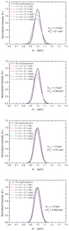Fig. 2. Comparison of evolution behavior for the down-Comptonization of the Gaussian line with hν0 = 1 keV between the classical Kompaneets equation and our extended equation. The evolution times T, hν0, and kTe are labeled in the figures. The blue and red lines represent the calculated results of the extended equation and the Kompaneets equation, respectively.

Fig. 3. Comparison of evolution behavior for the down-Comptonization of the Gaussian line with hν0 = 50 keV between the classical Kompaneets equation and our extended equation. The evolution times T, hν0, and kTe are labeled in the figures. The blue and red lines represent the calculated results of the extended equation and the Kompaneets equation, respectively.

As shown in Figs. 1, 2, and A.1–A.3, the line profiles in Compton evolution obtained by our extended equation Eq. (35) are nearly consistent with the ones obtained by the Kompaneets equation (Eq. (2)) when the energy of the line-photons is much lower than m_ec², i.e., hν₀ ≪ m_ec², including the cases hν₀ < kT_e and hν₀ > kT_e (see Figs. 1, A.1, and A.2; the differences between the corresponding curves are too small to be seen, except for Figs. A.2c and d), while the differences in the evolution behavior of the resultant line profiles for high-energy photons hν₀ > kT_e between Eqs. (2) and (35) are more obvious with the increasing of energy of the photons, especially for much higher energy photons hν₀ greater than several tens keV, even greater than several hundreds keV (see Figs. 3, A.4, and A.5). The big differences appear in Figs. 3, A.3, and A.4 for down-Comptonization (hν₀ > kT_e) because the term $\frac{14}{5}\frac{k{T}_{\mathrm{e}}}{m_{\mathrm{e}}{c}^2}x$ in Eq. (35) cannot be negligible, which can bring a much more significant contribution to the evolution behavior of the high-energy photons. On the other hand, even for the up-Comptonization process, if the temperature kT_e of electron is high enough (e.g., kT_e > 100 keV), more lower energy photons will be scattered to higher energy with the increase in the scattering time T, which also results in the difference of the evolution behavior between the extended Kompaneets equation and Kompaneets equation because the term $\frac{14}{5}\frac{k{T}_{\mathrm{e}}}{m_{\mathrm{e}}{c}^2}x$ in Eq. (35) becomes much more important for the Comptonization process of high-energy photons (e.g., see Figs. A.2c and d).

From Figs. 1, A.1, and A.2 we see the main evolution behavior of the line profile in up-Comptonization, which are as follows: (i) The peak positions of the line profiles are almost shifted to higher energies. We call this the “Compton blueshift” of the line. The longer the diffusion time T, the higher the line blueshift will be; (ii) The line width increases with T, which shows a diffusion behavior in the frequency space; (iii) The line profile becomes asymmetrical, steeper on the low-energy side and flatter on the high-energy side. Instead, from Figs. 2, 3, and A.4–A.6 we can summarize the main evolution features of the line profile in down-Comptonization as follows: (i) The peak position of the line is shifted to lower energies. We call this the “Compton redshift” of the line. The longer the diffusion time T, the higher the line redshift will be; (ii) The evolution behavior of the line profile has two distinctive manners, which are determined by the balance of the photon gas and the electron gas. If the difference between the line-photon energy hν₀ and the temperature kT_e of electron gas is not very large, from Figs. 2a, 3a, and A.4a–A.6a we see that the line width increases with T, which shows a diffusion behavior in the frequency space; instead, if the difference between hν₀ and kT_e is much larger, it seems that the line profile is just collectively shifted to lower energy side and the line width becomes slightly narrower (see Figs. 2c, 3c, and A.4c–A.6c); (iii) From Figs. 2a, 3a, and A.4a–A.6a we see that the line profiles also become asymmetrical, steeper on the low-energy side and flatter on the high-energy side, while for Figs. 2c, 3c, and A.4c–A.6c the line profiles are only slightly asymmetrical, steeper on both the low- and high-energy sides.

4. The Sunyaev-Zel’dovich effect correctness

The Sunyaev-Zel’dovich effect (SZE; Birkinshaw 1999; Carlstrom 2002; Rephaeli 1995; Challinor & Lasenby 1998) causes a change in the apparent brightness of the cosmic microwave background (CMB) when seen through the hot gas in a cluster of galaxies or any other reservoir of hot plasma. The SZE has a unique spectral signature that shows a decrease in the cosmic microwave background intensity at frequencies lower than around 218 GHz, and an increase in the intensity at higher frequencies. Clusters discovered by the SZE will determine their redshifts, mass content, and other properties. Just recently, an approach was proposed by Titarchuk & Lipunova (2019) to determine the optical depth and the electron temperature of a cluster by fitting the observation results of CMB through the plasma cloud.

The SZE usually employs the classical Kompaneets equation, with nonrelativistic treatments (Birkinshaw 1999). The unsimplified change in intensity is

$$\begin{array}{c}\hfill \mathrm{\Delta }I(\nu )=I_0{\tau }_{\mathrm{c}}\frac{k{T}_{\mathrm{e}}}{m_{\mathrm{e}}{c}^2}(1-\frac{T_{\mathrm{rad}}}{T_{\mathrm{e}}})\frac{X^4{e}^X}{{(e^X-1)}^2}[X\frac{e^X+1}{e^X-1}-4],\end{array}$$(39)

where the capital X, X ≡ hν/kT_rad, is different from the previous definition of the small letter x, x ≡ hν/kT_e; kT_rad is the equivalent temperature of photon gas (or radiation field) and $I_0=\frac{2h}{c^2}{\left(\frac{k{T}_{\mathrm{rad}}}{h}\right)}^3$; and τ_c = ∫N_e(r)σ_Tdr represents the optical depth (see I₀ and τ_c in Birkinshaw 1999; Molnar & Birkinshaw 1999), which is treated as a constant value here.

Recently, re-deriving the SZE from a more precise equation was tried by some authors (Challinor & Lasenby 1998; Itoh et al. 1998; Stebbins 1997). If using our extended Kompaneets equation Eq. (35), the modified SZE should be

$$\begin{array}{cc}\hfill \frac{\mathrm{\Delta }I(\nu )}{I_0{\tau }_{\mathrm{c}}}=& \frac{k{T}_{\mathrm{e}}}{m_{\mathrm{e}}{c}^2}(1-\frac{T_{\mathrm{rad}}}{T_{\mathrm{e}}})\frac{X^4{e}^X}{{(e^X-1)}^2}X\hfill \\ \hfill & \times [(1+\frac{14}{5}\frac{k{T}_{\mathrm{rad}}}{m_{\mathrm{e}}{c}^2}X)\frac{e^X+1}{e^X-1}-4-14\frac{k{T}_{\mathrm{rad}}}{m_{\mathrm{e}}{c}^2}]·\hfill \end{array}$$(40)

This modified SZE works for both cases, kT_rad < kT_e ≪ m_ec² and kT_e < kT_rad ≪ m_ec², so the comparison between kT_rad and kT_e is no longer required, which is an obvious advantage for this SZE, differing from the other modified SZEs. Comparing with Eq. (39), the two new terms $(1+\frac{14}{5}\frac{k{T}_{\mathrm{rad}}}{m_{\mathrm{e}}{c}^2}X)$ and $(-14\frac{k{T}_{\mathrm{rad}}}{m_{\mathrm{e}}{c}^2})$ are included in Eq. (40) and both depend on T_rad. However, for the CMB when passing through hot clusters where kT_e is greater than ∼1 keV, due to T_rad ≪ kT_e ≪ m_ec², the SZE Eqs. (39) and (40) are approximately identical:

$$\begin{array}{c}\hfill \frac{\mathrm{\Delta }I(\nu )}{I_0{\tau }_{\mathrm{c}}}=\frac{k{T}_{\mathrm{e}}}{m_{\mathrm{e}}{c}^2}\frac{X^4{e}^X}{{(e^X-1)}^2}[X\frac{e^X+1}{e^X-1}-4]·\end{array}$$(41)

In general, the temperatures of hot electron gas in clusters are much higher: kT_e ≃ 10 ∼ 20 keV. For example, for the A2163 Cluster, kT_e ≃ 12.4 ± 0.5 keV (Sarazin 1986; Rosati et al. 2002). Therefore, we compute the change in intensity of the blackbody spectrum with kT_rad = 2.37 × 10⁻⁷ keV (CMB) shown in Fig. 4 for thermal electron gas at kT_e = 5 keV, 10 keV, and 25 keV. Figure 4 shows that the discrepancy between the classical Kompaneets equation and our newly obtained Eq. (35) can be neglected for the Comptonization of CMB when passing through hot electron gas in the clusters, just because the radiation temperature of CMB is too low, kT_rad ≪ m_ec², for which Eq. (40) is almost exactly same as Eq. (39), i.e., the extended equation Eq. (35) returns to the Kompaneets equation Eq. (2).

Fig. 4. Change in intensity of the blackbody spectrum with kTrad = 2.35 × 10−7 keV (CMB) for thermal electron gas at kTe = 5 keV, 10 keV, and 25 keV as a function of dimensionless frequency X = hν/(kTrad), with scaling $I_0{\mathit{y}}_{\mathrm{c}}=\frac{2h}{c^2}{\left(\frac{k{T}_{\mathrm{rad}}}{h}\right)}^3{\mathit{y}}_{\mathrm{c}}$. The results obtained from the extended Kompaneets equation are shown as blue lines, while the red lines denote the results from the classical Kompaneets equation.

Although our extended Kompaneets equation obviously returns to the classical Kompaneets equation in the CMB condition, the differences of the evolution behavior between the classical Kompaneets equation and our new equation are outstanding for much higher temperature blackbody spectrum kT_rad > 10 keV when passing through the cold plasma surrounding the X-ray sources, shown in the following figures. Many authors have mentioned the radiation transfer process (i.e., the Comptonization) for X-ray and γ-ray photons including continuum spectra and emission lines in luminous sources, such as the compact X-ray binary sources, the supernova remnants, and the active galactic nuclei (Ross et al. 1978; Misra & Kembhavi 1998; Zhang et al. 2000; Wang et al. 2014; Adegoke et al. 2019; McCray & Hatchett 1975; Seward et al. 2012). In addition, the CMB is a pretty blackbody spectrum in our universe; the blackbody spectrum of X-rays is given by the Planckian formula in the following form, which is used in the obtainment of Eq. (39),

$$\begin{array}{c}\hfill I(\nu )=B_{\nu }(T_{\mathrm{rad}})=\frac{2h{\nu }^3}{c^2}·\frac{1}{exp[h\nu /k{T}_{\mathrm{rad}}]-1}·\end{array}$$(42)

To be specific, in the following model calculations, we take the typical temperatures of the X-ray blackbody spectrum, kT_rad = 1 keV, kT_rad = 5 keV, and kT_rad = 10 keV. In addition to calculating the up-Comptonization of X-ray blackbody spectra, we show the evolution behavior of blackbody spectrum under the extended Kompaneets equation and the classical Kompaneets equation, particularly in order to point out the distinct difference between the extended Kompaneets equation and the Kompaneets equation for dealing with the down-Comptonization of high-energy blackbody photons. The down-Comptonization of the X-ray blackbody spectrum will be the main focus; therefore, in the calculations we take kT_e ≤ kT_rad to ensure the possibility of down-Comptonization, particularly at the high-energy side of the blackbody spectrum. The initial condition now becomes

$$\begin{array}{c}\hfill n(x,0)=f(x)\sim \frac{1}{exp[x·(T_{\mathrm{e}}/T_{\mathrm{rad}})]-1}·\end{array}$$(43)

When kT_e < kT_rad, the calculated evolution behavior of blackbody spectrum for kT_rad = 1 keV, kT_rad = 5 keV, and kT_rad = 10 keV are shown in Figs. 5, 6, and A.8, respectively. If kT_e > kT_rad, the calculated evolution results for blackbody spectrum kT_rad = 1 keV, kT_rad = 5 keV, and kT_rad = 10 keV are respectively shown in Figs. A.6, A.9, and A.11. The blue lines represent the calculated results by our extended Kompaneets equation, while the red lines represent the calculated results by the classical Kompaneets equation, the temperatures of electron gas are labeled with different lines in each figure. At the same time, for comparison between the newly obtained equation and the Kompaneets equation, we also compute the change in intensity of the blackbody spectrum with kT_rad = 1 keV, kT_rad = 5 keV, and kT_rad = 10 keV using Eqs. (39) and (40) shown respectively in Figs. A.7, A.10, and 7 under the same temperatures of thermal electron gas as above. The spectral evolution behavior of blackbody spectrum are revealed as in the description of the Gaussian lines in Sect. 3. It should be noted that the big differences between the evolution behavior of high-energy blackbody photons (e.g., kT_rad > 10 keV) obtained by the extended Kompaneets equation and the original Kompaneets equation are clearly exhibited in Figs. 6 and A.11. Thus, we point out that we should use the extended Eq. (35) to deal with the Comptonization of high-energy photons including up-Comptonization and down-Comptonization instead of Eq. (2) because our equation is obtained under much looser conditions hν ≪ m_ec² and kT_e ≪ m_ec² than hν ≪ kT_e ≪ m_ec² for Eq. (2).

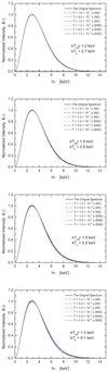Fig. 5. Comparison of evolution behavior for the down-Comptonization of X-ray blackbody spectrum with kTrad = 1 keV between the classical Kompaneets equation and our extended equation. The evolution times T, kTrad, and kTe are labeled in the figures. The blue and red lines represent the calculated results of the extended equation and the Kompaneets equation, respectively.

5. Conclusions and discussion

In this study, differing from the method used to obtain Eq. (4) by Liu et al. (2004), we present a new extended Kompaneets equation (35) by expanding the distribution function in Δp instead of Δν, which can be used to describe a more general Comptonization process, including down- and up-Comptonization, suitable for any case, hν ≪ kT_e, hν ≫ kT_e, and hν ∼ kT_e. The condition hν ≪ kT_e, under which the original Kompaneets equation (2) was derived, is no longer necessary for Eq. (35). The Kompaneets equation cannot give an accurate description of the down-Comptonization (hν ≫ kT_e) for X-rays and γ rays passing through the cold plasma, which is the most important radiative transfer process in high-energy astronomy (Ross et al. 1978; O’Dell 1986; Misra & Kembhavi 1998; Reynolds 2008; Kallman et al. 1979). However, our new extended equation will have potential applications in dealing with the Comptonization process in astrophysics including down- and up-Comptonization, especially for the down-Comptonization of hard X-rays and γ rays (see the calculated results in Sects. 3 and 4).

By Eq. (35) we give some typical numerical solutions including the evolution behavior of photons with Gaussian-line and blackbody spectra in X-ray and γ-ray astronomy, and compare them with the results of Kompaneets equation in Sects. 3 and 4. From these results, the significant changes of the emergent radiation spectrum from plasmas due to the affection of Comptonization have been shown in the calculated spectral curves (see figures in Sects. 3, 4, and Appendix A). Therefore, Comptonization as one of the most important radiative transfer processes in high-energy astrophysics should be noted (see Adegoke et al. 2019, and references therein). Above all things, our calculations show that for the photons with much lower energy than m_ec² (i.e., hν ≪ m_ec²) there is excellent consistency between the Compton-evolution spectra obtained by the use of the extended Kompaneets equation and the original Kompaneets equation, which confirms the correctness of our extended Kompaneets equation.

In addition, our calculations show that the change in the emergent spectrum in Comptonization, particularly in down-Comptonization, depends on the difference between $h\overline{\nu }$ and kT_e and on the scattering depth τ_s (or, equivalently, the diffusion timescale T): the larger the difference $h\overline{\nu }$ – kT_e, and/or the larger the depth τ_s (equivalently, the timescale T), the larger the change in the emergent spectrum. In addition, the Compton-evolution spectra for the blackbody spectrum and the Gaussian line have similar spectral evolution behavior. In particular, for both the blackbody spectrum and the Gaussian line, if only the energy of photons is high enough (e.g., hν > 10 keV), there are big differences between the evolution behavior obtained via the extended Kompaneets equation and via the original Kompaneets equation (see Figs. 3, 6, 7, A.4, and A.11), which indicates that we should use the extended Eq. (35) to deal with the Comptonization of high-energy photons including up-Comptonization and down-Comptonization instead of Eq. (2) because the term $\frac{14}{5}\frac{k{T}_{\mathrm{e}}}{m_{\mathrm{e}}{c}^2}x$ in Eq. (35) can bring a significant contribution to the evolution behavior for the high-energy photons. Therefore, Eq. (22) can be regarded as an important improvement of the original Kompaneets equation (2), particularly for hard X-ray and γ-ray astronomy.

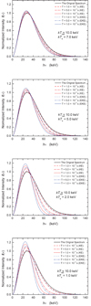Fig. 6. Comparison of evolution behavior for the down-Comptonization of X-ray blackbody spectrum with kTrad = 10 keV between the classical Kompaneets equation and our extended equation. The evolution times T, kTrad, and kTe are labeled in the figures. The blue and red lines represent the calculated results of the extended equation and the Kompaneets equation, respectively.

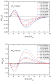Fig. 7. Change in intensity of the blackbody spectrum with kTrad = 10 keV under different temperatures of thermal electron gas calculated by use of Eqs. (39) and (40) as a function of dimensionless frequency X = hν/(kTrad), with scaling $I_0{\mathit{y}}_{\mathrm{c}}=\frac{2h}{c^2}{\left(\frac{k{T}_{\mathrm{rad}}}{h}\right)}^3{\mathit{y}}_{\mathrm{c}}$. kTrad and kTe are labeled in the figures. The results obtained under the extended Kompaneets equation and the classical Kompaneets equation are shown as blue and red lines, respectively.

The structure of Eq. (35) has two marked characteristics that can be regarded as a criterion of the correctness of our Eq. (35). First, it has the form $\frac{1}{x^2}\frac{\partial }{\partial x}\left\{x^4(1+\frac{14}{5}\frac{k{T}_{\mathrm{e}}}{m_{\mathrm{e}}{c}^2}x)[\frac{\partial n}{\partial x}+n(n+1)]\right\}$, which ensures the conservation of number of photons (see the conservation Eq. (28)). The invariance of the total number of photons is a basic requirement for the electron-photon scattering process. Second, Eq. (35) contains a factor $[\frac{\partial n}{\partial x}+n(n+1)]$, which ensures ∂n/∂t = 0 when the photon gas reaches the thermal equilibrium distribution n = (e^x − 1)⁻¹. This is also a necessary requirement for the correctness of this equation because the thermal equilibrium will inevitably be reached through the scattering and ∂n/∂t → 0, which implies that the diffusion finally stops. Ross et al. (1978) also noticed the restriction hν ≪ kT_e ≪ m_ec² of the original Kompaneets equation (2) and suggested an alternative equation to replace Eq. (2) to suit the case $h\overline{\nu }\gg k{T}_{\mathrm{e}}$. Their equation has the form $\frac{1}{x^2}\frac{\partial }{\partial x}\left\{x^4[n+(1+\frac{7}{10}\frac{k{T}_{\mathrm{e}}}{m_{\mathrm{e}}{c}^2}{x}^2)\frac{\partial n}{\partial x}]\right\}$, which is quite similar to Eq. (35), but deviates from the necessary form $[\frac{\partial n}{\partial x}+n(n+1)]$. According to their equation, the diffusion will never stop, i.e., ∂n/∂t ≠ 0 even when the thermal equilibrium, n = (e^x − 1)⁻¹, has been reached.

As a result, we note again that our extended Kompaneets equation obviously returns to the classical Kompaneets equation in the CMB condition (i.e., the Sunyaev-Zel’dovich effect (SZE)), and Eqs. (39) and (40) are approximately identical for CMB. However, just as indicated by many authors, Compton up-scattering of optical–UV seed photons into X-rays in the hot corona can provide a compelling explanation for the optical–UV–X-ray correlated variability seen in AGN and compact X-ray binaries (Ross et al. 1978; Zhang et al. 2000; Gaskell 2007; Breedt et al. 2010; Fabian et al. 2015; Buisson et al. 2018; Bonson et al. 2018; Adegoke et al. 2019). Recently, Adegoke et al. (2019) have argued that there is a UV to X-ray Comptonization delay in the narrow-line Seyfert 1 galaxy Mrk 493. Through the light variations in the UV emission preceding the variations in the X-ray emission based on ∼100 ks XMM-Newton observations of Mrk 493, they found that the UV emission leads by ∼5 ks relative to the X-ray emission. Then, they reported that the UV lead is consistent with the time taken by the UV photons to travel from the location of their origin in the accretion disk to the hot corona, and the time required for repeated inverse Compton scattering converting the UV photons into X-ray photons. In addition, for X-ray binaries, Zhang et al. (2000) have proposed the three-layered atmospheric structure in accretion disks around stellar-mass black holes. Also, the Comptonization process may be operating in these systems. Therefore, our extended equation will have potential applications for dealing with the Comptonization process in astrophysics including down- and up-Comptonization, especially for the down-Comptonization of hard X-rays and γ rays (see the calculated results in Sects. 3 and 4). In the future, we plan to investigate the Comptonization process in high-energy astrophysics, especially for X-ray and γ-ray astronomy.

Acknowledgments

We thank J. Ling and J. Evslin for fruitful discussions and suggestions. This work is partly supported by the Strategic Priority Research Program of Chinese Academy of Sciences, Grant No. XDB34030301. DL acknowledges support by the National Science Foundation of China (Grant Nos. U1631101, 11665022, 11233006), and the Shanghai Science and Technology Commission (Grant No. 16ZR1417200).

References

Appendix A: Additional figures

In this appendix we present the figures regarding the behavior of Compton evolution behavior of different spectra as a supplement to the main text, where the conclusions and discussions of Comptonization under various conditions are given. In Figs. A.1–A.5 we compare the evolution behavior of Gaussian line spectra with hν₀ = 1.0 keV, 10 keV for the up-Compotnization and hν₀ = 10 keV, 100 keV, 200 keV for the down-Comptonization. Moreover, Figs. A.6–A.11 show the Comptonization of X-ray blackbody spectra with kT_rad = 1.0 keV, 5.0 keV, 10 keV for both up- and down-Comptonization. The intensity changes obtained under classical and extended Kompaneets equations are also displayed here.

Fig. A.1. Comparison of evolution behavior for the up-Comptonization of the Gaussian line with hν0 = 1 keV between the classical Kompaneets equation and our extended equation. The evolution times T, hν0, and kTe are labeled in the figures. The blue and red lines represent the calculated results of the extended equation and the Kompaneets equation, respectively.

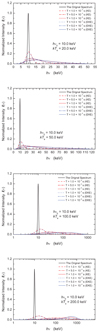Fig. A.2. Comparison of evolution behavior for the up-Comptonization of the Gaussian line with hν0 = 10 keV between the classical Kompaneets equation and our extended equation. The evolution times T, hν0, and kTe are labeled in the figures. The blue and red lines represent the calculated results of the extended equation and the Kompaneets equation, respectively.

Fig. A.3. Comparison of evolution behavior for the down-Comptonization of the Gaussian line with hν0 = 10 keV between the classical Kompaneets equation and our extended equation. The evolution times T, hν0, and kTe are labeled in the figures. The blue and red lines represent the calculated results of the extended equation and the Kompaneets equation, respectively.

Fig. A.4. Comparison of evolution behavior for the down-Comptonization of the Gaussian line with hν0 = 100 keV between the classical Kompaneets equation and our extended equation. The evolution times T, hν0, and kTe are labeled in the figures. The blue and red lines represent the calculated results of the extended equation and the Kompaneets equation, respectively.

Fig. A.5. Comparison of evolution behavior for the down-Comptonization of the Gaussian line with hν0 = 200 keV between the classical Kompaneets equation and our extended equation. The evolution times T, hν0, and kTe are labeled in the figures. The blue and red lines represent the calculated results of the extended equation and the Kompaneets equation, respectively.

Fig. A.6. Comparison of evolution behavior for the up-Comptonization of X-ray blackbody spectrum with kTrad = 1 keV between the classical Kompaneets equation and our extended equation. The evolution times T, kTrad, and kTe are labeled in the figures. The blue and red lines represent the calculated results of the extended equation and the Kompaneets equation, respectively.

Fig. A.7. Change in intensity of the blackbody spectrum with kTrad = 1 keV under different temperatures of thermal electron gas calculated by use of Eqs. (39) and (40) as a function of dimensionless frequency X = hν/(kTrad), with scaling $I_0{\mathit{y}}_{\mathrm{c}}=\frac{2h}{c^2}{\left(\frac{k{T}_{\mathrm{rad}}}{h}\right)}^3{\mathit{y}}_{\mathrm{c}}$. kTrad and kTe are labeled in the figures. The results obtained under the extended Kompaneets equation and the classical Kompaneets equation are shown as solid and red lines, respectively.

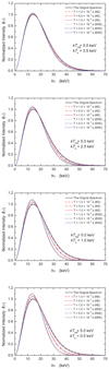Fig. A.8. Comparison of evolution behavior for the down-Comptonization of X-ray blackbody spectrum with kTrad = 5 keV between the classical Kompaneets equation and our extended equation. The evolution times T, kTrad, and kTe are labeled in the figures. The blue and red lines represent the calculated results of the extended equation and the Kompaneets equation, respectively.

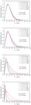Fig. A.9. Comparison of evolution behavior for the down-Comptonization of X-ray blackbody spectrum with kTrad = 5 keV between the classical Kompaneets equation and our extended equation. The evolution times T, kTrad, and kTe are labeled in the figures. The blue and red lines represent the calculated results of the extended equation and the Kompaneets equation, respectively.

Fig. A.10. Change in intensity of the blackbody spectrum with kTrad = 5 keV under different temperatures of thermal electron gas calculated by use of Eqs. (39) and (40) as a function of dimensionless frequency X = hν/(kTrad), with scaling $I_0{\mathit{y}}_{\mathrm{c}}=\frac{2h}{c^2}{\left(\frac{k{T}_{\mathrm{rad}}}{h}\right)}^3{\mathit{y}}_{\mathrm{c}}$. kTrad and kTe are labeled in the figures. The results obtained under the extended Kompaneets equation and the classical Kompaneets equation are shown as solid and red lines, respectively.

Fig. A.11. Comparison of evolution behavior for the up-Comptonization of X-ray blackbody spectrum with kTrad = 10 keV between the classical Kompaneets equation and our extended equation. The evolution times T, kTrad, and kTe are labeled in the figures. The blue and red lines represent the calculated results of the extended equation and the Kompaneets equation, respectively.

All Figures

	Fig. 1. Comparison of evolution behavior for the up-Comptonization of the Gaussian line with hν0 = 0.1 keV between the classical Kompaneets equation and our extended equation. The evolution times T, hν0, and kTe are labeled in the figures. The blue and red lines represent the calculated results of the extended equation and the Kompaneets equation, respectively.
In the text

	Fig. 2. Comparison of evolution behavior for the down-Comptonization of the Gaussian line with hν0 = 1 keV between the classical Kompaneets equation and our extended equation. The evolution times T, hν0, and kTe are labeled in the figures. The blue and red lines represent the calculated results of the extended equation and the Kompaneets equation, respectively.
In the text

	Fig. 3. Comparison of evolution behavior for the down-Comptonization of the Gaussian line with hν0 = 50 keV between the classical Kompaneets equation and our extended equation. The evolution times T, hν0, and kTe are labeled in the figures. The blue and red lines represent the calculated results of the extended equation and the Kompaneets equation, respectively.
In the text

Fig. 4. Change in intensity of the blackbody spectrum with kTrad = 2.35 × 10−7 keV (CMB) for thermal electron gas at kTe = 5 keV, 10 keV, and 25 keV as a function of dimensionless frequency X = hν/(kTrad), with scaling $I_0{\mathit{y}}_{\mathrm{c}}=\frac{2h}{c^2}{\left(\frac{k{T}_{\mathrm{rad}}}{h}\right)}^3{\mathit{y}}_{\mathrm{c}}$. The results obtained from the extended Kompaneets equation are shown as blue lines, while the red lines denote the results from the classical Kompaneets equation.

In the text

	Fig. 5. Comparison of evolution behavior for the down-Comptonization of X-ray blackbody spectrum with kTrad = 1 keV between the classical Kompaneets equation and our extended equation. The evolution times T, kTrad, and kTe are labeled in the figures. The blue and red lines represent the calculated results of the extended equation and the Kompaneets equation, respectively.
In the text

	Fig. 6. Comparison of evolution behavior for the down-Comptonization of X-ray blackbody spectrum with kTrad = 10 keV between the classical Kompaneets equation and our extended equation. The evolution times T, kTrad, and kTe are labeled in the figures. The blue and red lines represent the calculated results of the extended equation and the Kompaneets equation, respectively.
In the text

Fig. 7. Change in intensity of the blackbody spectrum with kTrad = 10 keV under different temperatures of thermal electron gas calculated by use of Eqs. (39) and (40) as a function of dimensionless frequency X = hν/(kTrad), with scaling $I_0{\mathit{y}}_{\mathrm{c}}=\frac{2h}{c^2}{\left(\frac{k{T}_{\mathrm{rad}}}{h}\right)}^3{\mathit{y}}_{\mathrm{c}}$. kTrad and kTe are labeled in the figures. The results obtained under the extended Kompaneets equation and the classical Kompaneets equation are shown as blue and red lines, respectively.

In the text

	Fig. A.1. Comparison of evolution behavior for the up-Comptonization of the Gaussian line with hν0 = 1 keV between the classical Kompaneets equation and our extended equation. The evolution times T, hν0, and kTe are labeled in the figures. The blue and red lines represent the calculated results of the extended equation and the Kompaneets equation, respectively.
In the text

	Fig. A.2. Comparison of evolution behavior for the up-Comptonization of the Gaussian line with hν0 = 10 keV between the classical Kompaneets equation and our extended equation. The evolution times T, hν0, and kTe are labeled in the figures. The blue and red lines represent the calculated results of the extended equation and the Kompaneets equation, respectively.
In the text

	Fig. A.3. Comparison of evolution behavior for the down-Comptonization of the Gaussian line with hν0 = 10 keV between the classical Kompaneets equation and our extended equation. The evolution times T, hν0, and kTe are labeled in the figures. The blue and red lines represent the calculated results of the extended equation and the Kompaneets equation, respectively.
In the text

	Fig. A.4. Comparison of evolution behavior for the down-Comptonization of the Gaussian line with hν0 = 100 keV between the classical Kompaneets equation and our extended equation. The evolution times T, hν0, and kTe are labeled in the figures. The blue and red lines represent the calculated results of the extended equation and the Kompaneets equation, respectively.
In the text

	Fig. A.5. Comparison of evolution behavior for the down-Comptonization of the Gaussian line with hν0 = 200 keV between the classical Kompaneets equation and our extended equation. The evolution times T, hν0, and kTe are labeled in the figures. The blue and red lines represent the calculated results of the extended equation and the Kompaneets equation, respectively.
In the text

	Fig. A.6. Comparison of evolution behavior for the up-Comptonization of X-ray blackbody spectrum with kTrad = 1 keV between the classical Kompaneets equation and our extended equation. The evolution times T, kTrad, and kTe are labeled in the figures. The blue and red lines represent the calculated results of the extended equation and the Kompaneets equation, respectively.
In the text

Fig. A.7. Change in intensity of the blackbody spectrum with kTrad = 1 keV under different temperatures of thermal electron gas calculated by use of Eqs. (39) and (40) as a function of dimensionless frequency X = hν/(kTrad), with scaling $I_0{\mathit{y}}_{\mathrm{c}}=\frac{2h}{c^2}{\left(\frac{k{T}_{\mathrm{rad}}}{h}\right)}^3{\mathit{y}}_{\mathrm{c}}$. kTrad and kTe are labeled in the figures. The results obtained under the extended Kompaneets equation and the classical Kompaneets equation are shown as solid and red lines, respectively.

In the text

	Fig. A.8. Comparison of evolution behavior for the down-Comptonization of X-ray blackbody spectrum with kTrad = 5 keV between the classical Kompaneets equation and our extended equation. The evolution times T, kTrad, and kTe are labeled in the figures. The blue and red lines represent the calculated results of the extended equation and the Kompaneets equation, respectively.
In the text

	Fig. A.9. Comparison of evolution behavior for the down-Comptonization of X-ray blackbody spectrum with kTrad = 5 keV between the classical Kompaneets equation and our extended equation. The evolution times T, kTrad, and kTe are labeled in the figures. The blue and red lines represent the calculated results of the extended equation and the Kompaneets equation, respectively.
In the text

Fig. A.10. Change in intensity of the blackbody spectrum with kTrad = 5 keV under different temperatures of thermal electron gas calculated by use of Eqs. (39) and (40) as a function of dimensionless frequency X = hν/(kTrad), with scaling $I_0{\mathit{y}}_{\mathrm{c}}=\frac{2h}{c^2}{\left(\frac{k{T}_{\mathrm{rad}}}{h}\right)}^3{\mathit{y}}_{\mathrm{c}}$. kTrad and kTe are labeled in the figures. The results obtained under the extended Kompaneets equation and the classical Kompaneets equation are shown as solid and red lines, respectively.

In the text

	Fig. A.11. Comparison of evolution behavior for the up-Comptonization of X-ray blackbody spectrum with kTrad = 10 keV between the classical Kompaneets equation and our extended equation. The evolution times T, kTrad, and kTe are labeled in the figures. The blue and red lines represent the calculated results of the extended equation and the Kompaneets equation, respectively.
In the text

References

- Adegoke, O., Dewangan, G. C., Pawar, P., et al. 2019, ApJ, 870, L13 [Google Scholar]
- Birkinshaw, M. 1999, Phys. Rep., 310, 97 [Google Scholar]
- Breedt, E., McHardy, I. M., Arevalo, P., et al. 2010, MNRAS, 403, 605 [Google Scholar]
- Bonson, K., Gallo, L. C., Wilkins, D. R., et al. 2018, MNRAS, 477, 3247 [Google Scholar]
- Buisson, D. J. K., Fabian, A. C., & Lohfink, A. M. 2018, MNRAS, 481, 4419 [Google Scholar]
- Carlstrom, J. E. 2002, ARA&A, 40, 643 [Google Scholar]
- Challinor, A., & Lasenby, A. 1998, ApJ, 499, 1 [Google Scholar]
- Chen, J. F., You, J. H., & Cheng, F. H. 1994, J. Phys. A: Math. Gen., 27, 2905 [Google Scholar]
- Deng, J. S., Chen, J. F., & You, J. H. 1998, Sci. China (Ser. A), 41, 10 [Google Scholar]
- Fabian, A. C., Nandra, K., Reynolds, C. S., et al. 1995, MNRAS, 277, L11 [Google Scholar]
- Fabian, A. C., Lohfink, A., Kara, E., et al. 2015, MNRAS, 451, 4375 [NASA ADS] [CrossRef] [Google Scholar]
- Felten, J. E., & Rees, M. J. 1972, A&A, 17, 226 [NASA ADS] [Google Scholar]
- Gaskell, C. M. 2007, Proc. ASP Conf. Ser., eds. L. C., Ho, & J.-M., Wang, 373, 596 [Google Scholar]
- Hua, X. M., Kazanas, D., & Titarchuk, L. G. 1997, ApJ, 482, L57 [Google Scholar]
- Illarionov, A. F., Kallman, T., McCray, R., et al. 1979, ApJ, 228, 279 [Google Scholar]
- Itoh, N., Kohyama, Y., & Nozawa, S. 1998, ApJ, 502, 7 [Google Scholar]
- Kallman, T., McCray, R., & Ross, R. R. 1979, ApJ, 228, 279 [Google Scholar]
- Kazanas, D., Hua, X. M., & Titarchuk, L. G. 1997, ApJ, 480, 735 [Google Scholar]
- Kompaneets, A. S. 1957, Sov. Phys. JETP, 4, 730 [Google Scholar]
- Kompaneets, A. S., & Eksper, Z. 1956, Teoret. Fiz., 31, 876 [Google Scholar]
- Liu, D. B., Chen, L., Ling, J. J., et al. 2004, A&A, 417, 381 [EDP Sciences] [Google Scholar]
- McCray, R., & Hatchett, S. 1975, ApJ, 199, 196 [Google Scholar]
- Misra, R., & Kembhavi, A. K. 1998, ApJ, 499, 205 [Google Scholar]
- Miyamoto, S. 1978, A&A, 63, 69 [Google Scholar]
- Molnar, S. M., & Birkinshaw, M. 1999, ApJ, 523, 78 [Google Scholar]
- O’Dell, S. L. 1986, PASP, 98, 140 [Google Scholar]
- Rephaeli, Y. 1995, ApJ, 445, 33 [Google Scholar]
- Reynolds, S. P. 2008, ARA&A, 46, 89 [Google Scholar]
- Rybicki, G. B., & Lightman, A. P. 1979, Radiative Processes in Astrophysics (New York: Wiley) [Google Scholar]
- Rosati, P., Borgani, S., & Norman, C. 2002, ARA&A, 40, 539 [NASA ADS] [CrossRef] [Google Scholar]
- Ross, R. R., Weaver, R., & McCray, R. 1978, ApJ, 219, 292 [Google Scholar]
- Sarazin, C. L. 1986, Rev. Mod. Phys., 58, 1 [NASA ADS] [CrossRef] [Google Scholar]
- Seward, F. D., Charles, P. A., Foster, D. L., et al. 2012, ApJ, 759, 123 [Google Scholar]
- Shakura, N. I., & Sunyaev, R. A. 1973, A&A, 24, 337 [NASA ADS] [Google Scholar]
- Stebbins, A. 1997, ArXiv e-prints [arXiv:astro-ph/9705178] [Google Scholar]
- Sunyaev, R. A., & Titarchuk, L. G. 1980, A&A, 86, 121 [NASA ADS] [Google Scholar]
- Sunyaev, R. A., & Titarchuk, L. G. 1985, A&A, 143, 374 [NASA ADS] [Google Scholar]
- Titarchuk, L. G. 1994, ApJ, 434, 570 [Google Scholar]
- Titarchuk, L. G., & Lipunova, G. V. 2019, ArXiv e-prints [arXiv:1906.07060] [Google Scholar]
- Treves, A., Morini, M., Chiappetti, L., et al. 1989, ApJ, 341, 733 [Google Scholar]
- Wang, J. M., Du, P., Hu, C., et al. 2014, ApJ, 793, 108 [Google Scholar]
- Zhang, S. N., Cui, W., Chen, W., et al. 2000, Science, 287, 1239 [Google Scholar]