| Issue |
A&A
Volume 649, May 2021
Gaia Early Data Release 3
|
|
|---|---|---|
| Article Number | A9 | |
| Number of page(s) | 19 | |
| Section | Celestial mechanics and astrometry | |
| DOI | https://doi.org/10.1051/0004-6361/202039734 | |
| Published online | 28 April 2021 | |
Gaia Early Data Release 3
Acceleration of the Solar System from Gaia astrometry★
1
Lohrmann Observatory, Technische Universität Dresden,
Mommsenstraße 13,
01062
Dresden,
Germany
2
Université Côte d’Azur, Observatoire de la Côte d’Azur, CNRS, Laboratoire Lagrange, Bd de l’Observatoire,
CS 34229,
06304
Nice Cedex 4,
France
3
Lund Observatory, Department of Astronomy and Theoretical Physics, Lund University,
Box 43,
22100
Lund,
Sweden
4
Astronomisches Rechen-Institut, Zentrum fôr Astronomie der Universität Heidelberg,
Mönchhofstr. 12-14,
69120
Heidelberg,
Germany
5
European Space Agency (ESA), European Space Astronomy Centre (ESAC), Camino bajo del Castillo, s/n, Urbanizacion Villafranca del Castillo, Villanueva de la Cañada,
28692
Madrid,
Spain
6
Vitrociset Belgium for European Space Agency (ESA), Camino bajo del Castillo, s/n, Urbanizacion Villafranca del Castillo, Villanueva de la Cañada,
28692
Madrid,
Spain
7
HE Space Operations BV for European Space Agency (ESA), Camino bajo del Castillo, s/n, Urbanizacion Villafranca del Castillo, Villanueva de la Cañada,
28692
Madrid,
Spain
8
Telespazio Vega UK Ltd for European Space Agency (ESA), Camino bajo del Castillo, s/n, Urbanizacion Villafranca del Castillo, Villanueva de la Cañada,
28692
Madrid,
Spain
9
Leiden Observatory, Leiden University,
Niels Bohrweg 2,
2333
CA
Leiden,
The Netherlands
10
INAF – Osservatorio astronomico di Padova,
Vicolo Osservatorio 5,
35122
Padova,
Italy
11
European Space Agency (ESA), European Space Research and Technology Centre (ESTEC),
Keplerlaan 1,
2201AZ
Noordwijk,
The Netherlands
12
Univ. Grenoble Alpes, CNRS, IPAG,
38000
Grenoble,
France
13
GEPI, Observatoire de Paris, Université PSL, CNRS,
5 Place Jules Janssen,
92190
Meudon,
France
14
Institute of Astronomy, University of Cambridge,
Madingley Road,
Cambridge
CB3 0HA,
UK
15
Department of Astronomy, University of Geneva,
Chemin des Maillettes 51,
1290
Versoix,
Switzerland
16
Aurora Technology for European Space Agency (ESA), Camino bajo del Castillo, s/n, Urbanizacion Villafranca del Castillo, Villanueva de la Cañada,
28692
Madrid,
Spain
17
Institut de Ciències del Cosmos (ICCUB), Universitat de Barcelona (IEEC-UB), Martí i Franquès 1,
08028
Barcelona,
Spain
18
CNES Centre Spatial de Toulouse,
18 avenue Edouard Belin,
31401
Toulouse Cedex 9,
France
19
Institut d’Astronomie et d’Astrophysique, Université Libre de Bruxelles CP 226, Boulevard du Triomphe,
1050
Brussels,
Belgium
20
F.R.S.-FNRS,
Rue d’Egmont 5,
1000
Brussels,
Belgium
21
INAF – Osservatorio Astrofisico di Arcetri,
Largo Enrico Fermi 5,
50125
Firenze,
Italy
22
Laboratoire d’astrophysique de Bordeaux, Univ. Bordeaux, CNRS, B18N, allée Geoffroy Saint-Hilaire,
33615
Pessac,
France
23
Max Planck Institute for Astronomy,
Königstuhl 17,
69117
Heidelberg,
Germany
24
Mullard Space Science Laboratory, University College London, Holmbury St Mary,
Dorking,
Surrey
RH5 6NT,
UK
25
INAF – Osservatorio Astrofisico di Torino,
Via Osservatorio 20,
10025
Pino Torinese (TO),
Italy
26
University of Turin, Department of Physics,
Via Pietro Giuria 1,
10125
Torino,
Italy
27
DAPCOM for Institut de Ciències del Cosmos (ICCUB), Universitat de Barcelona (IEEC-UB),
Martí i Franquès 1,
08028
Barcelona,
Spain
28
Royal Observatory of Belgium,
Ringlaan 3,
1180
Brussels,
Belgium
29
ALTEC S.p.a, Corso Marche,
79,
10146
Torino,
Italy
30
Department of Astronomy, University of Geneva,
Chemin d’Ecogia 16,
1290
Versoix,
Switzerland
31
Sednai Sàrl,
Geneva,
Switzerland
32
Gaia DPAC Project Office, ESAC, Camino bajo del Castillo, s/n, Urbanizacion Villafranca del Castillo,
Villanueva de la Cañada,
28692
Madrid,
Spain
33
SYRTE, Observatoire de Paris, Université PSL, CNRS, Sorbonne Université, LNE,
61 avenue de l’Observatoire
75014
Paris,
France
34
National Observatory of Athens, I. Metaxa and Vas. Pavlou, Palaia Penteli,
15236
Athens,
Greece
35
IMCCE, Observatoire de Paris, Université PSL, CNRS, Sorbonne Université, Univ. Lille,
77 av. Denfert-Rochereau,
75014
Paris,
France
36
INAF – Osservatorio Astrofisico di Catania,
Via S. Sofia 78,
95123
Catania,
Italy
37
Serco Gestión de Negocios for European Space Agency (ESA), Camino bajo del Castillo, s/n, Urbanizacion Villafranca del Castillo,
Villanueva de la Cañada,
28692
Madrid,
Spain
38
INAF – Osservatorio di Astrofisica e Scienza dello Spazio di Bologna,
Via Piero Gobetti 93/3,
40129
Bologna,
Italy
39
Institut d’Astrophysique et de Géophysique, Université de Liège,
19c, Allée du 6 Août,
4000
Liège,
Belgium
40
CRAAG – Centre de Recherche en Astronomie, Astrophysique et Géophysique,
Route de l’Observatoire Bp 63 Bouzareah
16340
Algiers,
Algeria
41
Institute for Astronomy, University of Edinburgh, Royal Observatory,
Blackford Hill,
Edinburgh
EH9 3HJ,
UK
42
ATG Europe for European Space Agency (ESA), Camino bajo del Castillo, s/n, Urbanizacion Villafranca del Castillo,
Villanueva de la Cañada,
28692
Madrid,
Spain
43
ETSE Telecomunicación, Universidade de Vigo,
Campus Lagoas-Marcosende,
36310
Vigo,
Galicia,
Spain
44
Université de Strasbourg, CNRS, Observatoire astronomique de Strasbourg,
UMR 7550, 11 rue de l’Université,
67000
Strasbourg,
France
45
Kavli Institute for Cosmology Cambridge, Institute of Astronomy,
Madingley Road,
Cambridge,
CB3 0HA,
USA
46
Department of Astrophysics, Astronomy and Mechanics, National and Kapodistrian University of Athens,
Panepistimiopolis, Zografos,
15783
Athens,
Greece
47
Observational Astrophysics, Division of Astronomy and Space Physics, Department of Physics and Astronomy, Uppsala University,
Box 516,
751 20
Uppsala,
Sweden
48
Leibniz Institute for Astrophysics Potsdam (AIP),
An der Sternwarte 16,
14482
Potsdam,
Germany
49
CENTRA, Faculdade de Ciências, Universidade de Lisboa,
Edif. C8, Campo Grande,
1749-016
Lisboa,
Portugal
50
Department of Informatics, Donald Bren School of Information and Computer Sciences, University of California,
5019 Donald Bren Hall,
92697-3440
CA
Irvine,
USA
51
Dipartimento di Fisica e Astronomia “Ettore Majorana”, Università di Catania,
Via S. Sofia 64,
95123
Catania,
Italy
52
CITIC, Department of Nautical Sciences and Marine Engineering, University of A Coruña, Campus de Elviña s/n,
15071,
A Coruña,
Spain
53
INAF – Osservatorio Astronomico di Roma,
Via Frascati 33,
00078
Monte Porzio Catone (Roma),
Italy
54
Space Science Data Center - ASI, Via del Politecnico SNC,
00133
Roma,
Italy
55
Department of Physics, University of Helsinki,
PO Box 64,
00014
Helsinki,
Finland
56
Finnish Geospatial Research Institute FGI,
Geodeetinrinne 2,
02430
Masala,
Finland
57
STFC, Rutherford Appleton Laboratory,
Harwell,
Didcot,
OX11 0QX,
UK
58
Institut UTINAM CNRS UMR6213, Université Bourgogne Franche-Comté, OSU THETA Franche-Comté Bourgogne, Observatoire de Besançon,
BP1615,
25010
Besançon Cedex,
France
59
HE Space Operations BV for European Space Agency (ESA),
Keplerlaan 1,
2201AZ,
Noordwijk,
The Netherlands
60
Dpto. de Inteligencia Artificial, UNED,
c/ Juan del Rosal 16,
28040
Madrid,
Spain
61
Applied Physics Department, Universidade de Vigo,
36310
Vigo,
Spain
62
Thales Services for CNES Centre Spatial de Toulouse,
18 avenue Edouard Belin,
31401
Toulouse Cedex 9,
France
63
Instituut voor Sterrenkunde, KU Leuven,
Celestijnenlaan 200D,
3001
Leuven,
Belgium
64
Department of Astrophysics/IMAPP, Radboud University,
PO Box 9010,
6500
GL
Nijmegen,
The Netherlands
65
CITIC – Department of Computer Science and Information Technologies, University of A Coruña,
Campus de Elviña s/n, 15071,
A Coruña,
Spain
66
Barcelona Supercomputing Center (BSC) - Centro Nacional de Supercomputación,
c/ Jordi Girona 29, Ed. Nexus II,
08034
Barcelona,
Spain
67
University of Vienna, Department of Astrophysics,
Türkenschanzstraße 17,
A1180
Vienna,
Austria
68
European Southern Observatory,
Karl-Schwarzschild-Str. 2,
85748
Garching,
Germany
69
Kapteyn Astronomical Institute, University of Groningen,
Landleven 12,
9747
AD
Groningen,
The Netherlands
70
School of Physics and Astronomy, University of Leicester,
University Road,
Leicester
LE1 7RH,
UK
71
Center for Research and Exploration in Space Science and Technology, University of Maryland Baltimore County,
1000
Hilltop Circle,
Baltimore
MD,
USA
72
GSFC - Goddard Space Flight Center,
Code 698, 8800 Greenbelt Rd,
20771
MD
Greenbelt,
USA
73
EURIX S.r.l.,
Corso Vittorio Emanuele II 61,
10128
Torino,
Italy
74
Harvard-Smithsonian Center for Astrophysics,
60 Garden St., MS 15,
Cambridge,
MA
02138,
USA
75
CAUP – Centro de Astrofisica da Universidade do Porto,
Rua das Estrelas,
Porto,
Portugal
76
SISSA – Scuola Internazionale Superiore di Studi Avanzati,
Via Bonomea 265,
34136
Trieste,
Italy
77
Telespazio for CNES Centre Spatial de Toulouse,
18 avenue Edouard Belin,
31401
Toulouse Cedex 9,
France
78
University of Turin, Department of Computer Sciences,
Corso Svizzera 185,
10149
Torino,
Italy
79
Departamento de Matemática Aplicada y Ciencias de la Computación, Universite de Cantabria,
ETS Ingenieros de Caminos, Canales y Puertos, Avda. de los Castros s/n,
39005
Santander,
Spain
80
Centro de Astronomía - CITEVA, Universidad de Antofagasta,
Avenida Angamos 601,
Antofagasta
1270300,
Chile
81
Vera C Rubin Observatory,
950 N. Cherry Avenue,
Tucson,
AZ
85719,
USA
82
Centre for Astrophysics Research, University of Hertfordshire,
College Lane,
AL10 9AB,
Hatfield,
UK
83
University of Antwerp, Onderzoeksgroep Toegepaste Wiskunde,
Middelheimlaan 1,
2020
Antwerp,
Belgium
84
INAF – Osservatorio Astronomico d’Abruzzo,
Via Mentore Maggini,
64100
Teramo,
Italy
85
Instituto de Astronomia, Geofìsica e Ciências Atmosféricas, Universidade de São Paulo,
Rua do Matão, 1226, Cidade Universitaria,
05508-900
São Paulo,
SP,
Brazil
86
Mésocentre de calcul de Franche-Comté, Université de Franche-Comté,
16 route de Gray,
25030
Besançon Cedex,
France
87
SRON, Netherlands Institute for Space Research,
Sorbonnelaan 2,
3584CA,
Utrecht,
The Netherlands
88
RHEA for European Space Agency (ESA), Camino bajo del Castillo, s/n, Urbanizacion Villafranca del Castillo,
Villanueva de la Cañada,
28692
Madrid,
Spain
89
ATOS for CNES Centre Spatial de Toulouse,
18 avenue Edouard Belin,
31401
Toulouse Cedex 9,
France
90
School of Physics and Astronomy, Tel Aviv University,
Tel Aviv
6997801,
Israel
91
Astrophysics Research Centre, School of Mathematics and Physics, Queen’s University Belfast,
Belfast
BT7 1NN,
UK
92
Centre de Données Astronomique de Strasbourg,
Strasbourg,
France
93
Université Côte d’Azur, Observatoire de la Côte d’Azur, CNRS, Laboratoire Géoazur, Bd de l’Observatoire,
CS 34229,
06304
Nice Cedex 4,
France
94
Max-Planck-Institut für Astrophysik,
Karl-Schwarzschild-Straße 1,
85748
Garching,
Germany
95
APAVE SUDEUROPE SAS for CNES Centre Spatial de Toulouse,
18 avenue Edouard Belin,
31401
Toulouse Cedex 9,
France
96
Área de Lenguajes y Sistemas Informáticos, Universidad Pablo de Olavide,
Ctra. de Utrera, km 1.
41013
Sevilla,
Spain
97
Onboard Space Systems, Luleå University of Technology,
Box 848,
981 28
Kiruna,
Sweden
98
TRUMPF Photonic Components GmbH,
Lise-Meitner-Straße 13,
89081
Ulm,
Germany
99
IAC - Instituto de Astrofisica de Canarias,
Via Láctea s/n,
38200
La Laguna S.C.,
Tenerife,
Spain
100
Department of Astrophysics, University of La Laguna,
Via Láctea s/n,
38200
La Laguna S.C.,
Tenerife,
Spain
101
Laboratoire Univers et Particules de Montpellier, CNRS Université Montpellier, Place Eugène Bataillon, CC72,
34095
Montpellier Cedex 05,
France
102
LESIA, Observatoire de Paris, Université PSL, CNRS, Sorbonne Université, Université de Paris,
5 Place Jules Janssen,
92190
Meudon,
France
103
Villanova University, Department of Astrophysics and Planetary Science,
800 E Lancaster Avenue,
Villanova PA
19085,
USA
104
Astronomical Observatory, University of Warsaw,
Al. Ujazdowskie 4,
00-478
Warszawa,
Poland
105
Laboratoire d’astrophysique de Bordeaux, Univ. Bordeaux, CNRS, B18N, allée Geoffroy Saint-Hilaire,
33615
Pessac,
France
106
Université Rennes, CNRS, IPR (Institut de Physique de Rennes) - UMR 6251,
35000
Rennes,
France
107
INAF – Osservatorio Astronomico di Capodimonte,
Via Moiariello 16,
80131
Napoli,
Italy
108
Niels Bohr Institute, University of Copenhagen,
Juliane Maries Vej 30,
2100
Copenhagen Ø,
Denmark
109
Las Cumbres Observatory,
6740 Cortona Drive Suite 102,
Goleta,
CA 93117,
USA
110
Astrophysics Research Institute, Liverpool John Moores University,
146 Brownlow Hill,
Liverpool
L3 5RF,
UK
111
IPAC, Mail Code 100-22, California Institute of Technology,
1200 E. California Blvd.,
Pasadena,
CA 91125,
USA
112
Jet Propulsion Laboratory, California Institute of Technology,
4800 Oak Grove Drive, M/S 169-327,
Pasadena,
CA 91109,
USA
113
IRAP, Université de Toulouse, CNRS, UPS, CNES,
9 Av. colonel Roche, BP 44346,
31028
Toulouse Cedex 4,
France
114
Konkoly Observatory, Research Centre for Astronomy and Earth Sciences, MTA Centre of Excellence,
Konkoly Thege Miklós út 15-17,
1121
Budapest,
Hungary
115
MTA CSFK Lendület Near-Field Cosmology Research Group, Konkoly Observatory, CSFK,
Konkoly Thege Miklós út 15-17,
1121
Budapest,
Hungary
116
ELTE Eötvös Loránd University, Institute of Physics,
1117, Pázmány Péter sétány 1A,
Budapest,
Hungary
117
Ruđer Bošković Institute,
Bijenička cesta 54,
10000
Zagreb,
Croatia
118
Institute of Theoretical Physics, Faculty of Mathematics and Physics, Charles University in Prague,
Czech Republic
119
INAF – Osservatorio Astronomico di Brera,
via E. Bianchi 46,
23807
Merate (LC),
Italy
120
AKKA for CNES Centre Spatial de Toulouse,
18 avenue Edouard Belin,
31401
Toulouse Cedex 9,
France
121
Departmento de Física de la Tierra y Astrofísica, Universidad Complutense de Madrid,
28040
Madrid,
Spain
122
Department of Astrophysical Sciences,
4 Ivy Lane, Princeton University,
Princeton NJ
08544,
USA
123
Departamento de Astrofísica, Centro de Astrobiología (CSIC-INTA), ESA-ESAC. Camino Bajo del Castillo s/n 28692 Villanueva de la Cañada,
Madrid,
Spain
124
naXys, University of Namur,
Rempart de la Vierge,
5000
Namur,
Belgium
125
EPFL – Ecole Polytechnique fédérale de Lausanne, Institute of Mathematics, Station 8 EPFL SB MATH SDS,
Lausanne,
Switzerland
126
H H Wills Physics Laboratory, University of Bristol,
Tyndall Avenue,
Bristol
BS8 1TL,
UK
127
Sorbonne Université, CNRS, UMR7095, Institut d’Astrophysique de Paris, 98bis bd. Arago,
75014
Paris,
France
128
Porter School of the Environment and Earth Sciences, Tel Aviv University,
Tel Aviv
6997801,
Israel
129
Laboratoire Univers et Particules de Montpellier, Université Montpellier,
Place Eugène Bataillon, CC72,
34095
Montpellier Cedex 05,
France
130
Faculty of Mathematics and Physics, University of Ljubljana,
Jadranska ulica 19,
1000
Ljubljana,
Slovenia
Received:
21
October
2020
Accepted:
30
November
2020
Abstract
Context. Gaia Early Data Release 3 (Gaia EDR3) provides accurate astrometry for about 1.6 million compact (QSO-like) extragalactic sources, 1.2 million of which have the best-quality five-parameter astrometric solutions.
Aims. The proper motions of QSO-like sources are used to reveal a systematic pattern due to the acceleration of the solar systembarycentre with respect to the rest frame of the Universe. Apart from being an important scientific result by itself, the acceleration measured in this way is a good quality indicator of the Gaia astrometric solution.
Methods. Theeffect of the acceleration was obtained as a part of the general expansion of the vector field of proper motions in vector spherical harmonics (VSH). Various versions of the VSH fit and various subsets of the sources were tried and compared to get the most consistent result and a realistic estimate of its uncertainty. Additional tests with the Gaia astrometric solution were used to get a better idea of the possible systematic errors in the estimate.
Results. Our best estimate of the acceleration based on Gaia EDR3 is (2.32 ± 0.16) × 10−10 m s−2 (or 7.33 ±0.51 km s−1 Myr−1) towards α = 269.1° ± 5.4°, δ = −31.6° ± 4.1°, corresponding to a proper motion amplitude of 5.05 ±0.35 μas yr−1. This is in good agreement with the acceleration expected from current models of the Galactic gravitational potential. We expect that future Gaia data releases will provide estimates of the acceleration with uncertainties substantially below 0.1 μas yr−1.
Key words: astrometry / proper motions / reference systems / Galaxy: kinematics and dynamics / methods: data analysis
Movie is only available at https://www.aanda.org
Corresponding author: S. A. Klioner, e-mail: This email address is being protected from spambots. You need JavaScript enabled to view it.
Deceased.
© ESO 2021
1 Introduction
It is well known that the velocity of an observer causes the apparent positions of all celestial bodies to be displaced in the direction of the velocity, an effect referred to as the aberration of light. If the velocity changes with time, that is if the observer is accelerated, the displacements also change, giving the impression of a pattern of proper motions in the direction of the acceleration. This effect can be exploited to detect the acceleration of the Solar System with respect to the rest frame of remote extragalactic sources.
Here we report on the first determination of the solar system acceleration using this effect in the optical domain, from Gaia observations. The paper is organised as follows. After some notes in Sect. 2 on the surprisingly long history of the subject, we summarise in Sect. 3 the astrometric signatures of an acceleration of the solar system barycentre with respect to the rest frame of extragalactic sources. Theoretical expectations of the acceleration of the Solar System are presented in Sect. 4. The selection of Gaia sources for the determination of the effect is discussed in Sect. 5. Section 6 presents the method, and the analysis of the data and a discussion of random and systematic errors are given in Sect. 7. Conclusions of this study as well as the perspectives for the future determination with Gaia astrometry are presented in Sect. 8. In Appendix A we discuss the general problem of estimating the length of a vector from the estimates of its Cartesian components.
2 From early ideas to modern results
2.1 Historical considerations
In 1833, John Pond, the Astronomer Royal at that time, sent to print the Catalogue of 1112 stars, reduced from observations made at the Royal Observatory at Greenwich (Pond 1833), the happy conclusion of a standard and tedious observatory work and a catalogue much praised for its accuracy (Grant 1852). At the end of his short introduction, he added a note discussing the Causes of Disturbance of the proper Motion of Stars, in which he considered the secular aberration resulting from the motion of the Solar System in free space, stating that,
So long as the motion of the Sun continues uniform and rectilinear, this aberration or distortion from their true places will be constant: it will not affect our observations; nor am I aware that we possess any means of determining whether it exist or not. If the motion of the Sun be uniformly accelerated, or uniformly retarded, […] [t]he effects of either of these suppositions would be, to produce uniform motion in every star according to its position,and might in time be discoverable by our observations, if the stars had no proper motions of their own […] But it is needless to enter into further speculation on questions that appear at present not likely to lead to the least practicalutility, though it may become a subject of interest to future ages.
This was a simple, but clever, realisation of the consequences of aberration. It was truly novel, and totally outside the technical capabilities of the time. The idea gained more visibility through the successful textbooks of the renowned English astronomer John Herschel, first in his Treatise of Astronomy (Herschel 1833, §612) and later in the expanded version Outlines of Astronomy (Herschel 1849, §862), both of which were printed in numerous editions. In the former, he referred directly to John Pond as the original source of this ‘very ingenious idea’, whereas in the latter the reference to Pond was dropped and the description of the effect looked unpromising:
This displacement, however, is permanent, and therefore unrecognizable by any phænomenon, so long as the solar motion remains invariable ; but should it, in the course of ages, alter its direction and velocity, both the direction and amount of the displacement in question would alter with it. The change, however, would become mixed up with other changes in the apparent proper motions of the stars, and it would seem hopeless to attempt disentangling them.
John Pond in 1833 wrote that the idea came to him ‘many years ago’ but did not hint at borrowing it from someone else. For such an idea to emerge, at least three devices had to be present in the tool kit of a practising astronomer: a deep understanding of aberration, enabled by James Bradley’s discovery of the effect in 1728; the secure proof that stars have proper motion, provided by the catalogue of Tobias Mayer in 1760; and the notion of the secular motion of the Sun towards the apex, established by William Herschel in 1783. Therefore Pond was probably the first, to our knowledge, who combined the aberration and the free motion of the Sun among the stars to draw the important observable consequence in terms of systematic proper motions. We have found no earlier mention, and had it been commonly known by astronomers much earlier, we would have found a mention in Lalande’s Astronomie (Lalande 1792), the most encyclopaedic treatise on the subject at the time.
References to the constant aberration due to the secular motion of the Solar System as a whole appear over the course of years in some astronomical textbooks (e.g. Ball 1908), but not in all of them with the hint that only a change in the apex would make it visible in the form of a proper motion. While the bold foresight of these forerunners was, by necessity, limited by their conception of the Milky Way and the Universe as a whole, both Pond and Herschel recognised that even with a curved motion of the Solar System, the effect on the stars from the change in aberration would be very difficult to separate from other sources of proper motion. This would remain true today if the stars of the Milky Way had been our only means to study the effect.
However, our current view of the hierarchical structure of the Universe puts the issue in a different and more favourable guise. The whole Solar System is in motion within the Milky Way and there are star-like sources, very far away from us, that do not share this motion. For them, the only source of apparent proper motion could be precisely the effect resulting from the change in the secular aberration. We are happily back to the world without proper motions contemplated by Pond, and we show in this paper that Gaia’s observations of extragalactic sources enable us to discern, for the first time in the optical domain, the signature of this systematic proper motion.
2.2 Recent work
Coming to the modern era, the earliest mention we have found of the effect on extragalactic sources is by Fanselow (1983) in the description of the JPL software package MASTERFIT for reducing Very Long Baseline Interferometry (VLBI) observations. There is a passing remark that the change in the apparent position of the sources from the solar system motion would be that of a proper motion of 6 μas yr−1, nearly two orders of magnitude smaller than the effect of source structure, but systematic. There is no detailed modelling of the effect, but at least this was clearly shown to be a consequence of the change in the direction of the solar system velocity vector in the aberration factor, worthy of further consideration. The description of the effect is given in later descriptions of MASTERFIT and also in some other publications of the JPL VLBI group (e.g. Sovers & Jacobs 1996; Sovers et al. 1998).
Eubanks et al. (1995) have a contribution in IAU Symposium 166 with the title Secular motions of the extragalactic radio-sources and the stability of the radio reference frame. This contains the first claim of seeing statistically significant proper motions in many sources at the level of 30 μas yr−1, about an order of magnitude larger than expected. This was unfortunately limited to an abstract, but the idea behind was to search for the effect discussed here. Proper motions of quasars were also investigated by Gwinn et al. (1997) in the context of search for low-frequency gravitational waves. The technique relied heavily on a decomposition on VSH (vector spherical harmonics), very similar to what is reported in the core of this paper.
Bastian (1995) rediscovered the effect in the context of the Gaia mission as it was planned at the time. He describes the effect as a variable aberration and stated clearly how it could be measured with Gaia using 60 bright quasars, with the unambiguous conclusion that ‘it seems quite possible that Gaia can significantly measure the galactocentric acceleration of the Solar System’. This was then included as an important science objective of Gaia in the mission proposal submitted to ESA in 2000 and in most early presentations of the mission and its expected science results (Perryman et al. 2001; Mignard 2002). Several theoretical discussions followed in relation to VLBI or space astrometry (Sovers et al. 1998; Kopeikin & Makarov 2006). Kovalevsky (2003) considered the effect on the observed motions of stars in our Galaxy, while Mignard & Klioner (2012) showed how the systematic use of the VSH on a large data sample like Gaia would permit a blind search of the acceleration without ad hoc model fitting. They also stressed the importance of solving simultaneously for the acceleration and the spin to avoid signal leakage from correlations.
With the VLBI data gradually covering longer periods of time, detection of the systematic patterns in the proper motions of quasars became a definite possibility, and in the last decade there have been several works claiming positive detections at different levels of significance. But even with 20 yr of data, the systematic displacement of the best-placed quasars is only ≃0.1 mas, not much larger than the noise floor of individual VLBI positions until very recently. So the actual detection was, and remains, challenging.
The first published solution by Gwinn et al. (1997), based on 323 sources, resulted in an acceleration estimate of (gx, gy, gz) = (1.9 ± 6.1, 5.4 ± 6.2, 7.5 ± 5.6) μas yr−1, not really above the noise level1. Then a first detection claim was by Titov et al. (2011), using 555 sources and 20 years of VLBI data. From the proper motions of these sources they found |g| = g = 6.4 ± 1.5 μas yr−1 for the amplitude of the systematic signal, compatible with the expected magnitude and direction. Two years later they published an improved solution from 34 years of VLBI data, yielding g = 6.4 ± 1.1 μas yr−1 (Titov & Lambert 2013). A new solution by Titov & Krásná (2018) with a global fit of the dipole on more than 4000 sources and 36 years of VLBI delays yielded g = 5.2 ± 0.2 μas yr−1, the best formal error so far, and a direction a few degrees off the Galactic centre. Xu et al. (2012) also made a direct fit of the acceleration vector as a global parameter to the VLBI delay observations, and found a modulus of g = 5.82 ± 0.32 μas yr−1 but with a strong component perpendicular to the Galactic plane.
The most recent VLBI estimate comes from a dedicated analysis of almost 40 years of VLBI observations, conducted as part of the preparatory work for the third version of the International Celestial Reference Frame (ICRF3). This dedicated analysis gave the acceleration g = 5.83 ± 0.23 μas yr−1 towards α = 270.2° ± 2.3°, δ = −20.2° ± 3.6° (Charlot et al. 2020). Based on this analysis, the value adopted for the ICRF3 catalogue is g = 5.8 μas yr−1, with the acceleration vector pointing toward the Galactic center, since the offset of the measured vector from the Galactic center was not deemed to be significant. The same recommendation was formulated by the Working Group on Galactic aberration of the International VLBI Service for Geodesy and Astrometry (IVS) which reported its work in MacMillan et al. (2019). This group was established to incorporate the effect of the galactocentric acceleration into the VLBI analysis with a unique recommended value. They make a clear distinction between the galactocentric component that may be estimated from Galactic kinematics, and the additional contributions due to the accelerated motion of the Milky Way in the intergalactic space or the peculiar acceleration of the Solar System in the Galaxy. They use the term ‘aberration drift’ for the total effect. Clearly the observations cannot separate the different contributions, neither in VLBI nor in the optical domain with Gaia.
To conclude this overview of related works, a totally different approach by Chakrabarti et al. (2020) was recently put forward, relying on highly accurate spectroscopy. With the performances of spectrographs reached in the search for extra-solar planets, on the level of 10 cm s−1, it is conceivable to detect the variation of the line-of-sight velocity of stars over a time baseline of at least ten years. This would be a direct detection of the Galactic acceleration and a way to probe the gravitational potential at ~kpc distances. Such a result would be totally independent of the acceleration derived from the aberration drift of the extragalactic sources and of great interest.
3 The astrometric effect of an acceleration
In the preceding sections we described aberration as an effect changing the ‘apparent position’ of a source. More accurately, it should be described in terms of the ‘proper direction’ to the source: this is the direction from which photons are seen to arrive, as measured in a physically adequate proper reference system of the observer (see, e.g. Klioner 2004, 2013). The proper direction, which we designate with the unit vector u, is what an astrometric instrument in space ideally measures.
The aberration of light is the displacement δu obtained when comparing the proper directions to the same source, as measured by two co-located observers moving with velocity v relative to each other. According to the theory of relativity (both special and general), the proper directions as seen by the two observers are related by a Lorentz transformation depending on the velocity v of one observer as measured bythe other. If δu is relatively large, as for the annual aberration, a rigorous approach to the computation is needed and also used, for example in the Gaia data processing (Klioner 2003). Here we are however concerned with small differential effects, for which first-order formulae (equivalent to first-order classical aberration) are sufficient. To first order in |v|∕c, where c is the speed of light, the aberrational effect is linear in v,
 (1)
(1)
Equation (1) is accurate to < 0.001 μas for |v| < 0.02 km s−1, and to < 1′′ for |v| < 600 km s−1 (see, however, below).
If v is changing with time, there is a corresponding time-dependent variation of δu, which affects all sources on the sky in a particular systematic way. A familiar example is the annual aberration, where the apparent positions seen from the Earth are compared with those of a hypothetical observer at the same location, but at rest with respect to the solar system barycentre. The annual variation of v∕c results in the aberrational effect that outlines a curve that is close to an ellipse with semi-major axis about 20′′ (the curve is not exactly an ellipse since the barycentric orbit of the Earth is not exactly Keplerian).
The motion with respect to the solar system barycentre is not the only conceivable source of aberrational effects. It is well known that the whole Solar System (that is, its barycentre) is in motion in the Galaxy with a velocity of about 248 km s−1 (Reid & Brunthaler 2020), and that its velocity with respect to the cosmic microwave background (CMB) radiation is about 370 km s−1 (Planck Collaboration III 2020). Therefore, if one compares the apparent positions of the celestial sources as seen by an observer at the barycentre of the Solar System with those seen by another observer at rest with respect to the Galaxy or the CMB, one would see aberrational differences up to ~ 171′′ or ~ 255′′, respectively – effects that are so big that they could be recognised by the naked eye (see Fig. 1 for an illustration of this effect). The first of these effects is sometimes called secular aberration. In most applications, however, there is no reason to consider an observer that is ‘even more at rest’ than the solar system barycentre. The reason is that this large velocity – for the purpose of astrometric observations and for their accuracies – can usually be considered as constant; and if the velocity is constant in size and direction, the principle of relativity imposes that the aberrational shift cannot be detected. In other words, without knowledge of the ‘true’ positions of the sources, one cannot reveal the constant aberrational effect on their positions.
However, the velocity of the Solar System is not exactly constant. The motion of the Solar System follows a curved orbit in the Galaxy, so its velocity vector is slowly changing with time. The secular aberration is therefore also slowly changing with time. Considering sources that do not participate in the galactic rotation (such as distant extragalactic sources), we see their apparent motions tracing out aberration ‘ellipses’ whose period is the galactic ‘year’ of ~ 213 million years – they are of course not ellipses owing to the epicyclic orbit of the Solar System (see Fig. 1). Over a few years, and even thousands of years, the tiny arcs described by the sources cannot be distinguished from the tangent of the aberration ellipse, and for the observer this is seen as a proper motion that can be called additional, apparent, or spurious:
 (2)
(2)
Here a = dv∕dt is the acceleration of the solar system barycentre with respect to the extragalactic sources. For a given source, this slow drift of the observed position is indistinguishable from its true proper motion. However, the apparent proper motion as given by Eq. (2) has a global dipolar structure with axial symmetry along the acceleration: it is maximal for sources in the direction perpendicular to the acceleration and zero for directions along the acceleration. This pattern is shown as a vector field in Fig. 2 in the case of the centripetal acceleration directed towards the galactic centre.
Because only the change in aberration can be observed, not the aberration itself, the underlying reference frame in Eq. (1) is irrelevant for the discussion. One could have considered another reference for the velocity, leading to a smaller or larger aberration, but the aberration drift would be the same and given by Eq. (2). Although this equation was derived by reference to the galactic motion of the Solar System, it is fully general and tells us that any accelerated motion of the Solar System with respect to the distant sources translates into a systematic proper-motion pattern of those sources, when the astrometric parameters are referenced to the solar system barycentre, as it is the case for Gaia. Using a rough estimate of the centripetal acceleration of the Solar System in its motion around the galactic centre, one gets the approximate amplitude of the spurious proper motions to be ~5 μas yr−1. A detailed discussion of the expected acceleration is given in Sect. 4.
It is important to realise that the discussion in this form is possible only when the first-order approximation given by Eq. (1) is used. It is the linearity of Eq. (1) in v that allows one, in this approximation, to decompose the velocity v in various parts and simply add individual aberrational effects from those components (e.g. annual and diurnal aberration in classical astrometry, or a constant part and a linear variation). In the general case of a complete relativistic description of aberration via Lorentz transformations, the second-order aberrational effects depend also on the velocity with respect to the underlying reference frame and can become large. However, when the astrometric parameters are referenced to the solar system barycentre, the underlying reference frame is at rest with respect to the barycentre and Eq. (2) is correct to a fractional accuracy of about |vobs |∕c ~ 10−4, where vobs is the barycentric velocity of the observer. While this is fully sufficient for the present and anticipated future determinations with Gaia, a more sophisticated modelling is needed, if a determination of the acceleration to better than ~0.01% is discussed in the future.
An alternative form of Eq. (2) is
 (3)
(3)
where μ = d(δu)∕dt is the proper motion vector due to the aberration drift and g = a∕c may be expressed in proper motion units, for example μas yr−1. Both vectors a and g are called ‘acceleration’ in the context of this study. Depending on the context, the acceleration may be given in different units, for example m s−2, μas yr−1, or km s−1 Myr−1 (1 μas yr−1 corresponds to 1.45343 km s−1 Myr−1 = 4.60566 × 10⁻¹¹ m s−2).
Equation (3) can be written in component form, using Cartesian coordinates in any suitable reference system and the associated spherical angles. For example, in equatorial (ICRS) reference system (x, y, z) the associated angles are right ascension and declination (α, δ). The components of the proper motion, μα*≡ μα cosδ and μδ, are obtained by projecting μ on the unit vectors eα and eδ in the directions of increasing α and δ at the position of the source (see Mignard & Klioner 2012, Fig. 1 and their Eqs. 64 and 65). The result is
 (4)
(4)
where (gx, gy, gz) are the equatorial components of g. A corresponding representation is valid in an arbitrary coordinate system. In this work, we use either equatorial (ICRS) coordinates (x, y, z) or galactic coordinates (X, Y, Z) and the corresponding associated angles (α, δ) and (l, b), respectively (see Sect. 4.4). Effects of the form in Eq. (4) are often dubbed ‘glide’ for the reasons explained inSect. 6.
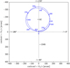 |
Fig. 1 Galactic aberration over 500 Myr for an observer looking towards Galactic north. The curve shows the apparent path of a hypothetical quasar, currently located exactly at the north galactic pole, as seen from the Sun (or solar system barycentre).The points along the path show the apparent positions after 0, 50, 100, …Myr due to the changing velocity of the Sun in its epicyclic orbit around the galactic centre. The point labelled GC is the position of the quasar as seen by an observer at rest with respect to the galactic centre. The point labelled CMB is the position as seen by an observer at rest with respect to the cosmic microwave background. The Sun’s orbit was computed using the potential model by McMillan (2017) (see also Sect. 4), with current velocity components derived from the references in Sect. 4.1. The Sun’s velocity with respect to the CMB is taken from Planck Collaboration III (2020). |
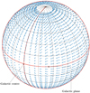 |
Fig. 2 Proper motion field of QSO-like objects induced by the centripetal galactic acceleration. There is no effect in the directions of the galactic centre and anti-centre, and amaximum in the plane passing through the galactic poles with nodes at 90–270° in galactic longitudes. The plot is in galactic coordinates with the Solar System at the centre of the sphere, and the vector field seen from the exterior of the sphere. Orthographic projection with viewpoint at l = 30°, b = 30° and an arbitrary scale for the vectors. See also an online movie. |
4 Theoretical expectations for the acceleration
This section is devoted to a detailed discussion of the expected gravitational acceleration of the Solar System. We stress, however, that the measurement of the solar system acceleration as outlined above and further discussed in subsequent sections is absolutely independent of the nature of the acceleration and the estimates given here.
As briefly mentioned in Sect. 3, the acceleration of the Solar System can, to first order, be approximated as the centripetal acceleration towards the Galactic centre which keeps the Solar System on its not-quite circular orbit around the Galaxy. In this section we quantify this acceleration and other likely sources of significant acceleration. The three additional parts which we consider are: (i) acceleration from the most significant non-axisymmetric components of the Milky Way, specifically the Galactic bar and spirals; (ii) the acceleration towards the Galactic plane, because the Milky Way is a flattened system and the Solar System lies slightly above the Galactic plane; and (ii) acceleration from specific objects, be they nearby galaxy clusters, local group galaxies, giant molecular clouds, or nearby stars.
For components of the acceleration associated with the bulk properties of the Galaxy we describe the acceleration in galactocentric cylindrical coordinates (R′, ϕ′, z′), where z′ = 0 for the Galactic plane, and the Sun is at z′ > 0). These are the natural model coordinates, and we convert into an acceleration in standard galactic coordinates (aX, aY, aZ) as a final step.
4.1 Centripetal acceleration
The distance and proper motion of Sagittarius A* – the super-massive black hole at the Galactic centre – has been measured with exquisite precision in recent years. Since this is expected to be very close to being at rest in the Galactic centre, the proper motion is almost entirely a reflex of the motion of the Sun around the Galactic centre. Its distance (GRAVITY Collaboration 2019) is

and its proper motion along the Galactic plane is − 6.411 ± 0.008 mas yr−1 (Reid & Brunthaler 2020). The Sun is not on a circular orbit, so we cannot directly translate the corresponding velocity into a centripetal acceleration. To compensate for this, we can correct the velocity to the ‘local standard of rest’ – the velocity that a circular orbit at d⊙−GC would have. This correction is12.24 ± 2 km s−1 (Schönrich et al. 2010), in the sense that the Sun is moving faster than a circular orbit at its position. Considered together this gives an acceleration of − 6.98 ± 0.12 km s−1 Myr−1 in the R′ direction. This corresponds to the centripetal acceleration of 4.80±0.08 μas yr−1 which is compatible with the values based on measurements of Galactic rotation, discussed for example by Reid et al. (2014) and Malkin (2014).
4.2 Acceleration from non-axisymmetric components
The Milky Way is a barred spiral galaxy. The gravitational force from the bar and spiral have important effects on the velocities of stars in the Milky Way, as has been seen in numerous studies using Gaia DR2 data (e.g. Gaia Collaboration 2018a). We separately consider acceleration from the bar and the spiral. Table 1 in Hunt et al. (2019) summarises models for the bar potential taken from the literature. From this, assuming that the Sun lies 30° away from the major axis of the bar (Wegg et al. 2015), most models give an acceleration in the negative ϕ′ direction of 0.04 km s−1 Myr−1, with one differing model attributed to Pérez-Villegas et al. (2017) which has a ϕ′ acceleration of 0.09 km s−1 Myr−1. The Portail et al. (2017) bar model, the potential from which is illustrated in Fig. 2 of Monari et al. (2019), is not included in the Hunt et al. (2019) table, but is consistent with the lower value.
The recent study by Eilers et al. (2020) found an acceleration from the spiral structure in the ϕ′ direction of 0.10 km s−1 Myr−1 in the opposite sense to the acceleration from the bar. Statistical uncertainties on this value are small, with systematic errors relating to the modelling choices dominating. This spiral strength is within the broad range considered by Monari et al. (2016), and we estimate the systematic uncertainty to be of order ± 0.05 km s−1 Myr−1.
4.3 Acceleration towards the Galactic plane
The baryonic component of the Milky Way is flattened, with a stellar disc which has an axis ratio of ~1:10 and a gas disc, with both H II and H2 components, which is even flatter. The Sun is slightly above the Galactic plane, with estimates of the height above the plane typically of the order 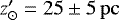 (Bland-Hawthorn & Gerhard 2016).
We use the Milky Way gravitational potential from McMillan (2017), which has stellar discs and gas discs based on literature results, to estimate this component of acceleration. We find an acceleration of 0.15± 0.03 km s−1 Myr−1 in the negative z′ direction, that is to say towards the Galactic plane. This uncertainty is found using only the uncertainty in d⊙−GC and  . We can estimate the systematic uncertainty by comparison to the model from McMillan (2011), which, among other differences, has no gas discs. In this case we find an acceleration of 0.13 ± 0.02 km s−1 Myr−1, suggesting that the uncertainty associated with the potential is comparable to that from the distance to the Galactic plane. For reference, if the acceleration were directed exactly at the Galactic centre we would expect an acceleration in the negative z′ direction of ~ 0.02 km s−1 Myr−1 due to the mentioned elevation of the Sun above the plane by 25 pc, see next subsection. Combined, this converts into an acceleration of (−6.98 ± 0.12, + 0.06 ± 0.05, − 0.15 ± 0.03) km s−1 Myr−1 in the (R′, ϕ′, z′) directions.
4.4 Transformation to standard galactic coordinates
For the comparison of this model expectation with the EDR3 observations we have to convert both into standard galactic coordinates (X, Y, Z) associated with galactic longitude and latitude (l, b). The standard galactic coordinates are defined by the transformation between the equatorial (ICRS) and galactic coordinates given in Sect. 1.5.3, Vol. 1 of ESA (1997) using three angles to be taken as exact quantities. In particular, the equatorial plane of the galactic coordinates is defined by its pole at ICRS coordinates (α = 192.85948°, δ = +27.12825°), and the origin of galactic longitude is defined by the galactic longitude of the ascending node of the equatorial plane of the galactic coordinates on the ICRS equator, which is taken to be lΩ = 32.93192°. This means that the point with galactic coordinates (l = 0, b = 0), that is the direction to the centre, is at (α ≃ 266.40499°, δ ≃−28.93617°).
The conversion of the model expectation takes into account the above-mentioned elevation of the Sun, leading to a rotation of the Z axis with respect to the z′ axis by (10.5 ± 2) arcmin, plus two sign flips of the axes’ directions. This leaves us with the final predicted value of (aX, aY, aZ) = (+6.98 ± 0.12, − 0.06 ± 0.05, − 0.13 ± 0.03) km s−1 Myr−1. We note that the rotation of the vertical axis is uncertain by about 2′, due to the uncertain values of d⊙−GC and Z⊙. This, however, gives an uncertainty of only 0.004 km s−1 Myr−1 in the predicted aZ.
We should emphasise that these transformations are purely formal ones. They should not be considered as strict in the sense that they refer the two vectors to the true attractive centre of the real galaxy. On the one hand, they assume that the standard galactic coordinates (X, Y, Z) represent perfect knowledge of the true orientation of the Galactic plane and the true location of the Galactic barycentre. On the other hand, they assume that the disc is completely flat, and that the inner part of the Galactic potential is symmetric (apart from the effects of the bar and local spiral structure discussed above). Both assumptions can easily be violated by a few arcmin. This can easily be illustrated by the position of the central black hole, Sgr A*. It undoubtedly sits very close in the bottom of the Galactic potential trough, by dynamical necessity. But that bottom needs not coincide with the barycentre of the Milky Way, nor with the precise direction of the inner galaxy’s force on the Sun2. In fact, the position of Sgr A* is off galactic longitude zero by − 3.3′, and off galactic latitude zero by − 2.7′. This latitude offset is only about a quarter of the 10.5′ correction derived from the Sun’s altitude above the plane.
Given the present uncertainty of the measured acceleration vector by a few degrees (see Table 2), these considerations about a few arcmin are irrelevant for the present paper. We mention them here as a matter of principle, to be taken into account in case the measured vector would ever attain a precision at the arcminute level.
4.5 Specific objects
Bachchan et al. (2016) provide in their Table 2 an estimate of the acceleration due to various extragalactic objects. We can use this table as an initial guide to which objects are likely to be important, however mass estimates of some of these objects (particularly the Large Magellanic Cloud) have changed significantly from the values quoted there.
We note first that individual objects in the Milky Way have a negligible effect. The acceleration from α Cen AB is ~ 0.004 km s−1 Myr−1, and that from any nearby giant molecular clouds is comparable or smaller. In the local group, the largest effect is from the Large Magellanic Cloud (LMC). A number of lines of evidence now suggest that it has a mass of (1− 2.5) × 1011 M⊙ (see Erkal et al. 2019 and references therein), which at a distance of 49.5± 0.5 kpc (Pietrzyński et al. 2019) gives an acceleration of 0.18 to 0.45 km s−1 Myr−1 with components (aX, aY, aZ) between (+0.025, − 0.148, − 0.098) and (+0.063, − 0.371, − 0.244) km s−1 Myr−1. We note therefore that the acceleration from the LMC is significantly larger than that from either the Galactic plane or non-axisymmetric structure.
The Small Magellanic Cloud is slightly more distant (62.8 ± 2.5 kpc; Cioni et al. 2000), and significantly less massive. It is thought that it has been significantly tidally stripped by the LMC (e.g. De Leo et al. 2020), so its mass is likely to be substantially lower than its estimated peak mass of ~ 7 × 10¹⁰ M⊙ (e.g. Read & Erkal 2019), but is hard to determine based on dynamical modelling. We follow Patel et al. (2020) and consider the range of possible masses (0.5−3) × 1010 M⊙, which gives an acceleration of 0.005 to 0.037 km s−1 Myr−1. Other local group galaxies have a negligible effect. M31, at a distance of 752 ± 27 kpc (Riess et al. 2012), with mass estimates in the range (0.7−2) × 1012 M⊙ (Fardal et al. 2013) imparts an acceleration of 0.005 to 0.016 km s−1 Myr−1. The Sagittarius dwarf galaxy is relatively nearby, and was once relatively massive, but has been dramatically tidally stripped to a mass ≲ 4 × 10⁸ M⊙ (Vasiliev & Belokurov 2020; Law & Majewski 2010), so provides an acceleration ≲ 0.003 km s−1 Myr−1. We note that this discussion only includes the direct acceleration that these local group bodies apply to the Solar System. They are expected to deform the Milky Way’s dark matter halo in a way that may also apply an acceleration (e.g. Garavito-Camargo et al. 2020).
We can, like Bachchan et al. (2016), estimate the acceleration due to nearby galaxy clusters from their estimated masses and distances. The Virgo cluster at a distance 16.5 Mpc (Mei et al. 2007) and a mass (1.4−6.3) × 1014 M⊙ (Ferrarese et al. 2012; Kashibadze et al. 2020) is the most significant single influence (0.002 to 0.010 km s−1 Myr−1). However, we recognise that the peculiar velocity of the Sun with respect to the Hubble flow has a component away from the Local Void, one towards the centre of the Laniakea supercluster, and others on larger scales that are not yet mapped (Tully et al. 2008, 2014), and that this is probably reflected in the acceleration felt on the solar system barycentre from large scale structure.
For simplicity we only add the effect of the LMC to the value given in Sect. 4.4. Adding our estimated ± 1σ uncertainties from the Galactic models to our full range of possible accelerations from the LMC, this gives an overall estimate of the expected range of (aX, aY, aZ) as (+6.89, − 0.16, − 0.20) to (+7.17, − 0.48, − 0.40) km s−1 Myr−1.
5 Selection of Gaia sources
5.1 QSO-like sources
Gaia Early Data Release 3 (EDR3; Gaia Collaboration 2021) provides high-accuracy astrometry for over 1.5 billion sources, mainly galactic stars. However, there are good reasons to believe that a few million sources are QSOs (quasi-stellar objects) and other extragalactic sources that are compact enough for Gaia to obtain good astrometric solutions. These sources are hereafter referred to as ‘QSO-like sources’. As explained in Sect. 5.2 it is only the QSO-like sources that can be used to estimate the acceleration of the Solar System.
Eventually, in later releases of Gaia data, we will be able to provide astrophysical classification of the sources and thus find all QSO-likesources based only on Gaia’s own data. EDR3 may be the last Gaia data release that needs to rely on external information to identify the QSO-like sources in the main catalogue of the release. To this end, a cross-match of the full EDR3 catalogue was performed with 17 external catalogues of QSOs and AGNs (active galactic nuclei). The matched sources were then further filtered to select astrometric solutions of sufficient quality in EDR3 and to have parallaxes and proper motions compatible with zero within five times the respective uncertainty. In this way, the contamination of the sample by stars is reduced, even though it may also exclude some genuine QSOs. It is important to recognise that the rejection based on significant proper motions does not interfere with the systematic proper motions expected from the acceleration, the latter being about two orders of magnitude smaller than the former. Various additional tests were performed to avoid stellar contamination as much as possible. As a result, EDR3 includes 1 614 173 sources thatwere identified as QSO-like; these are available in the Gaia Archive as the table agn_cross_id. The full details of the selectionprocedure, together with a detailed description of the resulting Gaia Celestial Reference Frame (Gaia-CRF3), will be published elsewhere (Gaia Collaboration, in prep.).
In Gaia EDR3 the astrometric solutions for the individual sources are of three different types (Lindegren et al. 2021a): (i) two-parameter solutions, for which only a mean position is provided; (ii) five-parameter solutions, for which the position (two coordinates), parallax, and proper motion (two components) are provided; (iii) six-parameter solutions, for which an astrometric estimate (the ‘pseudo-colour’) of the effective wavenumber3 is provided together with the five astrometric parameters.
Because of the astrometric filtering mentioned above, the Gaia-CRF3 sources only belong to the last two types of solutions: more precisely the selection comprises 1 215 942 sources with five-parameter solutions and 398 231 sources with six-parameter solutions. Table 1 gives the main characteristics of these sources. The Gaia-CRF3 sources with six-parameter solutions are typically fainter, redder, and have somewhat lower astrometric quality (as measured by the re-normalised unit weight error, RUWE) than those with five-parameter solutions4. Moreover, various studies of the astrometric quality of EDR3 (e.g. Fabricius et al. 2021; Lindegren et al. 2021a,b) have demonstrated that the five-parameter solutions generally have smaller systematic errors, at least for G > 16, that is for most QSO-like sources. In the following analysis we include only the 1 215 942 Gaia-CRF3 sources with five-parameter solutions.
Important features of these sources are displayed in Figs. 3–5. The distribution of the sources is not homogeneous on the sky, with densities ranging from 0 in the galactic plane to 85 sources per square degree, and an average density of 30 deg−2. The distribution of Gaia-CRF3 sources primarily reflects the sky inhomogeneities of the external QSO/AGN catalogues used to select the sources. In addition, to reduce the risk of source confusion in crowded areas, the only cross-matching made in the galactic zone ( , with b the galactic latitude) was with the VLBI quasars, for which the risk of confusion is negligible thanks to their accurate VLBI positions. One can hope that the future releases of Gaia-CRF will substantially improve the homogeneity and remove this selection bias (although a reduced source density at the galactic plane may persist due to the extinction in the galactic plane).
As discussed below, our method for estimating the solar system acceleration from proper motions of the Gaia-CRF3 sources involves an expansion of the vector field of proper motions in a set of functions that are orthogonal on the sphere. It is then advantageous if the data points are distributed homogeneously on the sky. However, as shown in Sect. 7.3 of Mignard & Klioner (2012), what is important is not the ‘kinematical homogeneity’ of the sources on the sky (how many per unit area), but the ‘dynamical homogeneity’: the distribution of the statistical weight of the data points over the sky (how much weight per unit area). This distribution is shown in Fig. 4.
For a reliable measurement of the solar system acceleration it is important to have the cleanest possible set of QSO-like sources. A significant stellar contamination may result in a systematic bias in the estimated acceleration (see Sect. 5.2). In this context the histograms of the normalised parallaxes and proper motions in Fig. 6 are a useful diagnostic. For a clean sample of extragalactic QSO-like sources one expects that the distributions of the normalised parallaxes and proper motions are Gaussian distributions with (almost) zero mean and standard deviation (almost) unity. Considering the typical uncertainties of the proper motions of over 400 μas yr−1 as given in Table 1 it is clear that the small effect of the solar system acceleration can be ignored in this discussion. The best-fit Gaussian distributions for the normalised parallaxes and proper motions shown by red lines on Fig. 6 indeed agree remarkably well with the actual distribution of the data. The best-fit Gaussian distributions have standard deviations of 1.052, 1.055 and 1.063, respectively for the parallaxes (ϖ), proper motions in right ascension (μα*), and proper motions in declination (μδ). Small deviations from Gaussian distributions can result both from statistical fluctuations in the sample and some stellar contaminations. One can conclude that the level of contaminations is probably very low (the logarithmic scale of the histograms should be noted).
Characteristics of the Gaia-CRF3 sources.
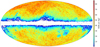 |
Fig. 3 Distribution of the Gaia-CRF3 sources with five-parameter solutions. The plot shows the density of sources per square degree computed from the source counts per pixel using HEALPix of level 6 (pixel size ≃0.84 deg2). This and following full-sky maps use a Hammer–Aitoff projection in galactic coordinates with l = b = 0 at the centre, north up, and l increasing from right to left. |
 |
Fig. 4 Distribution of the statistical weights of the proper motions of the Gaia-CRF3 sources with five-parameter solutions. Statistical weight is calculated as the sum of
|

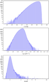 |
Fig. 5 Histograms of some important characteristics of the Gaia-CRF3 sources with five-parameter solutions. From top to bottom: G magnitudes, colours represented by the effective wavenumber νeff (see footnote 3), and the astrometric quality indicator RUWE (see footnote 4). |
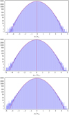 |
Fig. 6 Distributions of the normalised parallaxes ϖ∕σϖ
(upper panel), proper motions in right ascension |


5.2 Stars of our Galaxy
The acceleration of the Solar System affects also the observed proper motions of stars, albeit in a more complicated way than for the distant extragalactic sources5. Here it is however masked by other, much larger effects, and this section is meant to explain why it is not useful to look for the effect in the motions of galactic objects.
The expected size of the galactocentric acceleration term is of the order of 5 μas yr−1 (Sect. 4). The galactic rotation and shear effects are of the order of 5–10 mas yr−1, that is over a thousand times bigger. In the Oort approximation they do not contain a glide-like component, but any systematic difference between the solar motion and the bulk motion of some stellar population produces a glide-like proper-motion pattern over the whole sky. Examples of this are the solar apex motion (pointing away from the apex direction in Hercules, α ≃ 270°, δ ≃ 30°) and the asymmetric drift of old stars (pointing away from the direction of rotation in Cygnus, α ≃ 318°, δ ≃ 48°). Since these two directions – by pure chance – are only about 40° apart on the sky, the sum of their effects will be in the same general direction.
But both are distance dependent, which means that the size of the glide strongly depends on the stellar sample used. The asymmetric drift is, in addition, age dependent. Both effects attain the same order of magnitude as the Oort terms at a distance of the order of 1 kpc. That is, like the Oort terms they are of the order of a thousand times bigger than the acceleration glide. Because of this huge difference in size, and the strong dependence on the stellar sample, it is in practice impossible to separate the tiny acceleration effect from the kinematic patterns.
Some post-Oort terms in the global galactic kinematics (e.g. a non-zero second derivative of the rotation curve) can produce a big glide component, too. And, more importantly, any asymmetries of the galactic kinematics at the level of 0.1% can create glides in more or less random directions and with sizes far above the acceleration term. Examples are halo streams in the solar vicinity, the tip of the long galactic bar, the motion of the disc stars through a spiral wave crest, and so on.
For all these reasons it is quite obvious that there is no hope to discern an effect of 5 μas yr−1 amongst chaotic structures of the order of 10 mas yr−1 in stellar kinematics. In other words, we cannot use galactic objects to determine the glide due to the acceleration of the Solar System.
As a side remark we mention that there is a very big (≃ 6 mas yr−1) direct effect of the galactocentric acceleration in the proper-motion pattern of stars on the galactic scale: it is not a glide but the global rotation which is represented by the minima in the well-known textbook double wave of the proper motions μl* in galactic longitude l as function of l. But this is of no relevance in connection with the present study.
6 Method
One can think of a number of ways to estimate the acceleration from a set of observed proper motions. For example, one could directly estimate the components of the acceleration vector by a least-squares fit to the proper motion components using Eq. (4). However, if there are other large-scale patterns present in the proper motions, such as from a global rotation, these other effects could bias the acceleration estimate, because they are in general not orthogonal to the acceleration effect for the actual weight distribution on the sky (Fig. 4).
We prefer to use a more general and more flexible mathematical approach with vector spherical harmonics (VSH). For a given set of sources, the use of VSH allows us to mitigate the biases produced by various large-scale patterns, thus bringing a reasonable control over the systematic errors. The theory of VSH expansions of arbitrary vector fields on thesphere and its applications to the analysis of astrometric data were discussed in detail by Mignard & Klioner (2012). We use the notations and definitions given in that work. In particular, to the vector field of proper motions μ(α, δ) = μα* eα + μδ eδ (where eα and eδ are unit vectors in the local triad as in Fig. 1 of Mignard & Klioner 2012) we fit the following VSH representation:
 (5)
(5)
Here Tlm(α, δ) and Slm (α, δ) are the toroidal and spheroidal VSH of degree l and order m, tlm and slm are the corresponding coefficients of the expansion (to be fitted to the data), and the superscripts ℜ and ℑ denote the real and imaginary parts of the corresponding complex quantities, respectively. In general, the VSHs are defined as complex functions and can represent complex-valued vector fields, but the field of proper motions is real-valued and the expansion in Eq. (5) readily uses the symmetry properties of the expansion, so that all quantities in Eq. (5) are real. The definitions and various properties of Tlm (α, δ) and Slm (α, δ), as well as an efficient algorithm for their computation, can be found in Mignard & Klioner (2012).
The main goal of this work is to estimate the solar system acceleration described by Eq. (4). As explained in Mignard & Klioner (2012), a nice property of the VSH expansion is that the first-order harmonics with l = 1 represent a global rotation (the toroidal harmonics T1m) and an effect called ‘glide’ (the spheroidal harmonics S1m). Glide has the same mathematical form as the effect of acceleration given by Eq. (4). One can demonstrate (Sect. 4.2 in Mignard & Klioner 2012) that
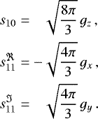 (6)
(6)
In principle, therefore, one could restrict the model to l = 1. However, as already mentioned, the higher-order VSHs help to handle the effects of other systematic signals. The parameter lmax in Eq. (5) is the maximal order of the VSHs that are taken into account in the model and is an important instrument for analysing systematic signals in the data: by calculating a series of solutions for increasing values of lmax, one probes how much the lower-order terms (and in particular the glide terms) are affected by higher-order systematics.
With the L2 norm, the VSHs Tlm(α, δ) and Slm(α, δ) form an orthonormal set of basis functions for a vector field on a sphere. It is also known that the infinite set of these basis functions is complete on S2. The VSHs can therefore represent arbitrary vector fields. Just as in the case of scalar spherical harmonics, the VSHs with increasing order l represent signals of higher spatial frequency on the sphere. VSHs of different orders and degrees are orthogonal only if one has infinite number of data points homogeneously distributed over the sphere. For a finite number of points and/or an inhomogeneous distribution the VSHs are not strictly orthogonal and have a non-zero projection onto each other. This means that the coefficients  ,
,  ,
,  and
and  are correlated when working with observational data. The level of correlation depends on the distribution of the statistical weight of the data over the sphere, which is illustrated by Fig. 4 for the source selection used in this study. For a given weight distribution there is a upper limit on the lmax that can be profitably used in practical calculations. Beyond that limit the correlations between the parameters become too high and the fit becomes useless. Numerical tests show that for our data selection it is reasonable to have lmax ≲ 10, for which correlations are less than about 0.6 in absolute values.
Projecting Eq. (5) on the vectors eα and eδ of the local triad one gets two scalar equations for each celestial source with proper motions μα* and μδ. For k sources this gives 2k observation equations for 2lmax(lmax + 2) unknowns to be solved for using a standard least-squares estimator. The equations should be weighted using the uncertainties of the proper motions  and
and  . It is also advantageous to take into account, in the weight matrix of the least-squares estimator, the correlation ρμ between μα* and μδ of a source. Thiscorrelation comes from the Gaia astrometric solution and is published in the Gaia catalogue for each source. The correlations between astrometric parameters of different sources are not exactly known and no attempt to account for these inter-source correlations was undertaken in this study.
It is important that the fit is robust against outliers, that is sources that have proper motions significantly deviating from the model in Eq. (5). Peculiar proper motions can be caused by time-dependent structure variation of certain sources (some but not all such sources have been rejected by the astrometric tests at the selection level). Outlier elimination also makes the estimates robust against potentially bad, systematically biased astrometric solutions of some sources. The outlier detection is implemented (Lindegren 2018) as an iterative elimination of all sources for which a measure of the post-fit residuals of the corresponding two equations exceed the median value of that measure computed for all sources by some chosen factor κ ≥ 1, called clip limit. As the measure X of the weighted residuals for a source we choose the post-fit residuals Δμα* and Δμδ of the corresponding two equations for μα* and μδ for the source, weighted by the full covariance matrix of the proper motion components:
![Mathematical equation: \begin{eqnarray*} X^2&=& \begin{bmatrix}\Delta\mu_{\alpha*} & \Delta\mu_{\delta}\end{bmatrix} \begin{bmatrix}\sigma_{\mu_{\alpha*}}^2 & \rho_{\mu}\sigma_{\mu_{\alpha*}}\sigma_{\mu_{\delta}}\\ \rho_{\mu}\sigma_{\mu_{\alpha*}}\sigma_{\mu_{\delta}} & \sigma_{\mu_{\delta}}^2\end{bmatrix}^{-1} \begin{bmatrix}\Delta\mu_{\alpha*}\\ \Delta\mu_{\delta}\end{bmatrix}\nonumber\\[6pt] &=&\frac{1}{1-\rho_{\mu}^2}\left[\left(\frac{\Delta\mu_{\alpha*}}{\sigma_{\mu_{\alpha*}}}\right)^2 -2\rho_{\mu}\left(\frac{\Delta\mu_{\alpha*}}{\sigma_{\mu_{\alpha*}}}\right)\left(\frac{\Delta\mu_{\delta}}{\sigma_{\mu_{\delta}}}\right) +\left(\frac{\Delta\mu_{\delta}}{\sigma_{\mu_{\delta}}}\right)^2\right]\,. \end{eqnarray*}](/articles/aa/full_html/2021/05/aa39734-20/aa39734-20-eq17.png) (7)
(7)
At each iteration the least-squares fit is computed using only the sources that were not detected as outliers in the previous iterations; the median of X is however always computed over the whole set of sources. Iteration stops when the set of sources identified as outliers is stable6. Identification of a whole source as an outlier and not just a single component of its proper motion (for example, accepting μα* and rejecting μδ) makes more sense from the physical point of view and also makes the procedure independent of the coordinate system.
It is worth recording here that the angular covariance function Vμ (θ), defined by Eq. (17) of Lindegren et al. (2018), also contains information on the glide, albeit only on its magnitude |g|, not the direction. Vμ (θ) quantifies the covariance of the proper motion vectors μ as a function of the angular separation θ on the sky. Figure 14 of Lindegren et al. (2021a) shows this function for Gaia EDR3, computed using the same sample of QSO-like sources with five-parameter solutions as used in the present study (but without weighting the data according to their uncertainties). Analogous to the case of scalar fields on a sphere (see Sect. 5.5 of Lindegren et al. 2021a), Vμ (θ) is related to the VSH expansion of the vector field μ(α, δ). In particular, the glide vector g gives a contribution of the form
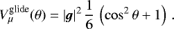 (8)
(8)
Using this expression and the Vμ(θ) of Gaia EDR3we obtain an estimate of |g| in reasonable agreement with the results from the VSH fit discussed in the next section. However, it is obvious from the plot in Lindegren et al. (2021a) that the angular covariance function contains other large-scale components that could bias this estimate as they are not included in the fit. This reinforces the argument made earlier in this section, namely that the estimation of the glide components from the proper motion data should not be done in isolation, but simultaneously with the estimation of other large-scale patterns. This is exactly what is achieved by means of the VSH expansion.
7 Analysis
The results for the three components of the glide vector are shown in Fig. 7. They have been obtained by fitting the VSH expansion in Eq. (5) for different lmax to the proper motions of the 1 215 942 Gaia-CRF3 sources with five-parameter solutions. The corresponding spheroidal VSH parameters with l = 1 were transformed into the Cartesian components of the glide using Eq. (6). Figure 7 displays both the equatorial components (gx, gy, gz) and the galactic components (gX, gY, gZ) of the glide vector. The equatorial components were derived directly using the equatorial proper motions published in the Gaia Archive. The galactic components can be derived either by transforming the equatorial components of the glide and their covariance matrix to galactic coordinates, or from a direct VSH fits using the proper motions and covariances in galactic coordinates. We have verified that the two procedures give strictly identical results.
One can see that starting from lmax = 3 the estimates are stable and generally deviate from each other by less than the corresponding uncertainties. The deviation of the results for lmax < 3 from those of higher lmax shows that the higher-order systematics in the data need to be taken into account, although their effect on the glide is relatively mild. We conclude that it is reasonable to use the results for lmax = 3 as the best estimates of the acceleration components.
The unit weight error (square root of the reduced chi-square) of all these fits, and of all those described below, is about 1.048. The unit weight error calculated with all VSH terms set to zero is also 1.048 (after applying the same outlier rejection procedure as for the fits), which merely reflects the fact that the fitted VSH terms are much smaller than the uncertainties of the individual proper motions. The unit weight error is routinely used to scale up the uncertainties of the fit. However, a more robust method of bootstrap resampling was used to estimate the uncertainties (see below).
To further investigate the influence of various aspects of the data and estimation procedure, the following tests were done. Fits including VSH components of degree up to lmax = 40 were made. They showed that the variations of the estimated acceleration components remain at the level of a fraction of the corresponding uncertainties, which agrees with random variations expected for the fits with high lmax. The fits in Fig. 7 used the clip limit κ = 3, which rejected about 3800 of the 1 215 942 sources as outliers (the exact number depends on lmax). Fits with different clip limits κ (including fits without outlier rejection, corresponding to κ = ∞) were tried, showing that the result for the acceleration depends on κ only at a level of a quarter of the uncertainties. Finally, we checked that the use of the correlations ρμ between the proper motion components for each source in the weight matrix of the fit influences the acceleration estimates at a level of ~0.1 of the uncertainties. This should be expected since the correlations ρμ for the 1 215 942 Gaia-CRF3 sources are relatively small (the distribution of ρμ is reasonably close to normal with zero mean and standard deviation 0.28).
Analysis of the Gaia DR3 astrometry has revealed systematic errors depending on the magnitude and colour of the sources (Lindegren et al. 2021a,b). To check how these factors influence the estimates, fits using lmax = 3 were made for sources splitby magnitude and colour. Figure 8 shows the acceleration components estimated for subsets of different mean G magnitude. The variation of the components with G is mild and the estimates are compatible with the estimates from the full data set (shown as horizontal colour bands) within their uncertainties. Figure 9 is a corresponding plot for the split by colour, as represented by the effective wavenumber νeff. Again one can conclude that the estimates from the data selections in colour agree with those from the full data set within their corresponding uncertainties.
It should be noted that the magnitude and colour selections are not completely independent since the bluer QSO-like sources tend to be fainter than the redder ones. Moreover, the magnitude and colour selections are less homogeneous on the sky than the full set of sources (for example owing to the Galactic extinction and reddening). However, we conclude that the biases in the acceleration estimates, due to magnitude- and colour-dependent effects in the Gaia DR3 astrometry, are below the formal uncertainties for the full sample.
Another possible cause of biases in the Gaia data is charge transfer inefficiency (CTI) in the detectors (e.g. Crowley et al. 2016). A detailed simulation of plausible CTI effects unaccounted for in the Gaia data processing for Gaia DR3 showed that the estimated glide is remarkably resilient to the CTI and may be affected only at a level below 0.1 μas yr−1 – at most a quarter of the quoted uncertainty.
Our selection of Gaia sources cannot be absolutely free from stellar contaminants. As discussed in Sect. 5.2, stars in our Galaxy have very large glide components in the vector field of their proper motions. This means that even a small stellar contamination could bias our estimate of the solar system acceleration. One can hope that the mechanism of outlier elimination used in the VSH fit in this work (see Sect. 6) helps to eliminate at least some of the most disturbing stellar-contamination sources. It is, however, worth to investigate the possible biases by direct simulation. By construction, the stellar contaminants in our list of QSO-like sources must have five-parameter solutions in Gaia DR3 that satisfy the selection criteria discussed in Sect. 5.1 and Gaia Collaboration (in prep.). It is therefore of interest to investigate the sample of sources obtained by making exactly the same selection of Gaia DR3 sources, but without the cross-match to the external QSO/AGN catalogues. There are a total of 23.6 million such sources in Gaia DR3, including the 1.2 million (5.2%) included in Gaia-CRF3. Most of them are stars in our Galaxy, but one also sees stars in nearby dwarf galaxies, globular clusters, and bright stars in other galaxies. Applying the VSH method to this sample gives a glide of about 360 μas yr−1 in a direction within a few degrees of (l, b) = (270°, 0°), that is roughly opposite to the direction of motion of the Sun in the Galaxy. This glide has obviously nothing to do with the acceleration of the Solar System (see Sect. 5.2) and its precise value is irrelevant. However, it is very relevant that it is practically perpendicular to the glide obtained from the QSO-like sample, for it means that a (small) stellar contamination will not significantly alter the magnitude of the glide |g|. It could however bias the direction of the observed glide towards (l, b) = (270°, 0°), that is mainly in galactic longitude. We do not see a clear sign of this in our estimates (the estimated direction is within one σ from the Galactic centre) and we therefore conclude that the effect of a possible stellar contamination in Gaia-CRF3 is negligible for the claimed estimate of the solar system acceleration.
Finally, it should be remembered that systematic errors in the Gaia ephemeris may also bias the estimate of the solar system acceleration. The standard astrometric parameters in the Gaia astrometric solution are defined for a fictitious observer located in the ‘solar system barycentre’. The latter is effectively defined by the Gaia ephemeris in the Barycentric Celestial Reference Frame (BCRS; Soffel et al. 2003; Klioner 2003) that is used in the data processing. In particular, Gaia’s barycentric velocity is used to transform the observations from the proper frame of Gaia to the reference frame at rest with respect to the solar system barycentre (Klioner 2004). Systematic errors in the Gaia ephemeris may result in systematic errors in the astrometric parameters. In particular, a systematic error in the Gaia velocity, corresponding to a non-zero average acceleration error over the time interval of the observations (about 33 months for Gaia EDR3), will produce the same systematic error in the measured solar system acceleration.
The barycentric ephemeris of Gaia is obtained by combining the geocentric orbit determination, made by the Gaia Mission Operations Centre at the European Space Operations Centre (ESOC) using various Doppler and ranging techniques, with a barycentric ephemeris of the Earth7. For the latter, the INPOP10e planetary ephemerides (Fienga et al. 2016) were used in Gaia EDR3. The errors in the geocentric orbit have very different characteristics from those of the planetary ephemerides, and the two contributions need to be considered separately. For the geocentric part, one can rule out an acceleration bias greater than about 2 × 10⁻¹³ m s−2 persisting over the 33 months, because it would produce an offset in the position of Gaia of the order of a km, well above the accuracy obtained by the ranging. For the barycentric ephemeris of the Earth, we can obtain an order-of-magnitude estimate of possible systematics by comparing the INPOP10e ephemerides with the latest version, INPOP19a (Fienga et al. 2019), which will be used for Gaia DR4. Averaged over 33 months, the difference in the acceleration of the Earth between the two versions is of the order of 10−12 m s−2, that is about 0.5% of the observed (and expected) acceleration of the solar system barycentre. These differences in the Earth ephemeris come from improvements in the dynamical modelling of the Solar System and new observational data resulting in more accurate determination of the parameters of the solar system bodies. One can expect that the process of improvement will continue and involve, in particular, more objects in the outer Solar System that can potentially influence the definition of the solar system barycentre. For example, the hypothetical Planet Nine would have an effect of at most 5 × 10⁻¹³ m s−2 (Fienga et al. 2020). Taking all these aspects into account, we conclude that plausible systematic errors in the barycentric ephemeris of Gaia are too small, by at least two orders of magnitude, to invalidate our result. Nevertheless, special care should be taken for this source of systematic errors when considerably more accurate measurements of the solar system acceleration – for example from a combination of the Gaia and GaiaNIR data (Hobbs et al. 2016) – will become available.
The various tests and arguments reported above strengthen our confidence in the final results, which are summarised in Table 2. Both the equatorial and galactic components are given with their uncertainties and correlations.The uncertainties were estimated by bootstrap resampling (Efron & Tibshirani 1994), which in our case increased the uncertainties from the fit (already inflated by the unit weight error) by factors of 1.05 to 1.08. As shown already in Fig. 7, the direction of the measured acceleration is very close to the Galactic centre. This is also illustrated in Fig. 10, which shows the directions obtained in the bootstrap resampling.
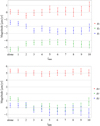 |
Fig. 7 Equatorial (upper panel) and galactic (lower panel) components of the solar system acceleration for fits with different maximal VSH order lmax (‘alone’ means that the three glide components were fitted with no other VSH terms). The error bars represent ± 1σ uncertainties. |
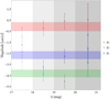 |
Fig. 8 Equatorial components of the acceleration and their uncertainties for four intervals of G magnitude: G ≤ 18 mag (29 200 sources), 18 < G ≤ 19 mag (146 614 sources), 19 < G ≤ 20 mag (490 161 sources), and G > 20 mag (549 967 sources). The horizontal colour bands visualise the values and uncertainties (the height corresponds to twice the uncertainty) of the corresponding components computed from the whole data set. |
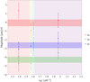 |
Fig. 9 Equatorial components of the acceleration and their uncertainties for four intervals of the colour represented by the effective wavenumber νeff used in Gaia DR3 astrometry. The quartiles of the νeff distribution for the sources considered in this study are used as the boundaries of the νeff intervals so that each interval contains about 304 000 sources. The horizontal colour bands visualise the values and uncertainties (the height corresponds to twice the uncertainty) of the corresponding components computed from the whole data set. |
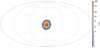 |
Fig. 10 Visualising the error ellipse of the estimated direction of the acceleration estimate in galactic coordinates. The plot is a density map of the directions from 550 000 bootstrap resampling experiments. The colour scale is logarithmic. |
Principal results of this work: equatorial and galactic components of the estimated acceleration of the Solar System, with uncertainties and correlations.
8 Conclusions and prospects
The exquisite quality of the Gaia DR3 astrometry together with a careful selection of the Gaia-CRF3 sources (Sect. 5.1) have allowed us to detect the acceleration of the Solar System with respect to the rest frame of the remote extragalactic sources, with a relative precision better than 10%. The stability of the derived estimates was extensively checked by numerous experiments as discussed in Sect. 7. The consistency of the results support the overall claim of a significant detection. We note that our estimate of the solar system acceleration agrees with the theoretical expectations from galactic dynamics (Sect. 4) within the corresponding uncertainties.
We stress that the detection of the solar system acceleration in the Gaia astrometry does not require any dedicated astrometric solution. The astrometric data used in this work to detect the acceleration and analyse its properties are those of the astrometric solution published in Gaia EDR3.
Although the relative accuracy obtained in the estimate is very satisfactory for this data release, it is at this stage impossible to tell whether there are acceleration contributions from other components than the motion of the Solar System in the Milky Way. As discussed in Sect. 4, even this contribution is complex and cannot be modelled with sufficient certainty to disentangle the different contributions.
We can ask ourselves what should be expected from Gaia in the future. The astrometric results in Gaia EDR3 are based only on 33 months of data, while the future Gaia DR4 will be based on about 66 months of data and the final Gaia DR5 may use up to 120 months of data. Since the effect of the acceleration is equivalent to proper motions, the random uncertainty of its measurement improves with observational time T as T−3∕2. Therefore, we can expect that the random errors of the acceleration estimated in Gaia DR4 and Gaia DR5 could go down by factors of about 0.35 and 0.15, respectively.
But random error is just one side of the story. What has made this solution possible with Gaia EDR3, while it was not possible with the Gaia DR2 data, is the spectacular decrease of the systematic errors in the astrometry. To illustrate this point, the glide determined from the Gaia-CRF2 data (Sect. 3.3 in Gaia Collaboration 2018b) was at the level of 10 μas yr−1 per component, much higher than a solution strictly limited by random errors. With the Gaia EDR3 we have a random error on each proper motion of about ≃ 400 μas yr−1 and just over 1 million sources. So one could hope to reach 0.4 μas yr−1 in the formal uncertainty of the glide components, essentially what is now achieved. In future releases, improvement for the solar system acceleration will come both from the better random errors and the reduced systematic errors, although only the random part can be quantified with some certainty. In the transition from Gaia DR2 to Gaia EDR3 a major part of the gain came from the diminishing of systematic errors.
The number of QSO-like sources that can become available in future Gaia data releases is another interesting aspect. In general, a reliable answer is not known. Two attempts (Shu et al. 2019; Bailer-Jones et al. 2019) to find QSO-like sources in Gaia DR2 data ended up with about 2.7 million sources each (and even more together). Although an important part of those catalogues did not show the level of reliability we require for Gaia-CRF3, one can hope that the number of QSO-like sources with Gaia astrometry will be doubled in the future compared with Gaia DR3. Taking all these aspects into account, it is reasonable to hope for the uncertainty of the acceleration to reach the level of well below 0.1 μas yr−1 in the future Gaia releases.
Considering the expected accuracy, an interesting question here is if we could think of any other effects that would give systematic patterns in the proper motions of QSO-like sources at the level of the expected accuracy. Such effects are indeed known (a good overview of these effects can be found e.g. in Bachchan et al. 2016). One such effect is the ‘cosmological proper motion’ (Kardashev 1986), or ‘secular extragalactic parallax’ (Paine et al. 2020), caused by the motion of the Solar System with respect to the rest frame of the CMB at a speed of 370 km s−1 ≃ 78 au yr−1 towards the point with galactic coordinates l = 264.02°, b = 48.25° (Planck Collaboration III 2020; see also Sect. 3). This gives a reflex proper motion of 78 μas yr−1 × (1 Mpc∕d)sinβ, where d is the distance to the object and β is the angle between the object and the direction of motion (Bachchan et al. 2016). The effect is analogous to the systematic proper motions of nearby stars caused by the apex motion of the Sun (Sect. 5.2), and like it decreases with the inverse distance to the sources. At a redshift of 0.2 the systematic proper motion should be about 0.1 μas yr−1 at right angle to the solar motion. However, only a few thousand QSO-like objects can be expected at such small redshifts, and, as discussedfor example by Paine et al. (2020), the effect is muddled by the peculiar velocities of the objects and deviations of their bulk motions from the Hubble flow due to the gravitational interactions with large-scale structures. It therefore remains questionable if this systematic proper motion will become accessible to Gaia in the future.
Another secular shift of the positions of extragalactic sources comes from the light bending in the gravitational field of the Galaxy, which depends (among other things) on the angle between the source and the Galactic centre. The motion of the Solar System in the Galaxy results in a slow variation of this angle, which causes a variation of the light bending. This will be seen as a proper motion of the extragalactic source. The effect is independent of the distance to the source (as long as it is far away from the Milky Way), but depends on its position on the sky according to the details of the Galactic potential. The VSH technique used in this work seems to be very well suited for disentangling this effect from that of the solar system acceleration.
Movie
Movie associated with Fig. 2. Access Supplementary Material
Acknowledgements
This work has made use of data from the European Space Agency (ESA) mission Gaia (https://www.cosmos.esa.int/gaia), processed by the Gaia Data Processing and Analysis Consortium (DPAC, https://www.cosmos.esa.int/web/gaia/dpac/consortium). Funding for the DPAC has been provided by national institutions, in particular the institutions participating in the Gaia Multilateral Agreement. This work presents results from the European Space Agency (ESA) space mission Gaia. Gaia data are being processed by the Gaia Data Processing and Analysis Consortium (DPAC). Funding for the DPAC is provided by national institutions, in particular the institutions participating in the Gaia MultiLateral Agreement (MLA). The Gaia mission website is https://www.cosmos.esa.int/gaia. The Gaia archive website is https://archives.esac.esa.int/gaia. The Gaia mission and data processing have financially been supported by, in alphabetical order by country: the Algerian Centre de Recherche en Astronomie, Astrophysique et Géophysique of Bouzareah Observatory; the Austrian Fonds zur Förderung der wissenschaftlichen Forschung (FWF) Hertha Firnberg Programme through grants T359, P20046, and P23737; the BELgian federal Science Policy Office (BELSPO) through various PROgramme de Développement d’Expériences scientifiques (PRODEX) grants and the Polish Academy of Sciences - Fonds Wetenschappelijk Onderzoek through grant VS.091.16N, and the Fonds de la Recherche Scientifique (FNRS); the Brazil-France exchange programmes Fundação de Amparo à Pesquisa do Estado de São Paulo (FAPESP) and Coordenação de Aperfeicoamento de Pessoal de Nível Superior (CAPES) - Comité Français d’Evaluation de la Coopération Universitaire et Scientifique avec le Brésil (COFECUB); the National Science Foundation of China (NSFC) through grants 11573054 and 11703065 and the China Scholarship Council through grant 201806040200; the Tenure Track Pilot Programme of the Croatian Science Foundation and the École Polytechnique Fédérale de Lausanne and the project TTP-2018-07-1171 ’Mining the Variable Sky’, with the funds of the Croatian-Swiss Research Programme; the Czech-Republic Ministry of Education, Youth, and Sports through grant LG 15010 and INTER-EXCELLENCE grant LTAUSA18093, and the Czech Space Office through ESA PECS contract 98058; the Danish Ministry of Science; the Estonian Ministry of Education and Research through grant IUT40-1; the European Commission’s Sixth Framework Programme through the European Leadership in Space Astrometry (ELSA) Marie Curie Research Training Network (MRTN-CT-2006-033481), through Marie Curie project PIOF-GA-2009-255267 (Space AsteroSeismology & RR Lyrae stars, SAS-RRL), and through a Marie Curie Transfer-of-Knowledge (ToK) fellowship (MTKD-CT-2004-014188); the European Commission’s Seventh Framework Programme through grant FP7-606740 (FP7-SPACE-2013-1) for the Gaia European Network for Improved data User Services (GENIUS) and through grant 264895 for the Gaia Research for European Astronomy Training (GREAT-ITN) network; the European Research Council (ERC) through grants 320360 and 647208 and through the European Union’s Horizon 2020 research and innovation and excellent science programmes through Marie Skłodowska-Curie grant 745617 as well as grants 670519 (Mixing and Angular Momentum tranSport of massIvE stars – MAMSIE), 687378 (Small Bodies: Near and Far), 682115 (Using the Magellanic Clouds to Understand the Interaction of Galaxies), and 695099 (A sub-percent distance scale from binaries and Cepheids – CepBin); the European Science Foundation (ESF), in the framework of the Gaia Research for European Astronomy Training Research Network Programme (GREAT-ESF); the European Space Agency (ESA) in the framework of the Gaia project, through the Plan for European Cooperating States (PECS) programme through grants for Slovenia, through contracts C98090 and 4000106398/12/NL/KML for Hungary, and through contract 4000115263/15/NL/IB for Germany; the Academy of Finland and the Magnus Ehrnrooth Foundation; the French Centre National d’Etudes Spatiales (CNES), the Agence Nationale de la Recherche (ANR) through grant ANR-10-IDEX-0001-02 for the ‘Investissements d’avenir’ programme, through grant ANR-15-CE31-0007 for project ‘Modelling the Milky Way in the Gaia era’ (MOD4Gaia), through grant ANR-14-CE33-0014-01 for project ‘The Milky Way disc formation in the Gaia era’ (ARCHEOGAL), and through grant ANR-15-CE31-0012-01 for project ‘Unlocking the potential of Cepheids as primary distance calibrators’ (UnlockCepheids), the Centre National de la Recherche Scientifique (CNRS) and its SNO Gaia of the Institut des Sciences de l’Univers (INSU), the ‘Action Fédératrice Gaia’ of the Observatoire de Paris, the Région de Franche-Comté, and the Programme National de Gravitation, Références, Astronomie, et Métrologie (GRAM) of CNRS/INSU with the Institut National de Physique (INP) and the Institut National de Physique nucléaire et de Physique des Particules (IN2P3) co-funded by CNES; the German Aerospace Agency (Deutsches Zentrum für Luft- und Raumfahrt e.V., DLR) through grants 50QG0501, 50QG0601, 50QG0602, 50QG0701, 50QG0901, 50QG1001, 50QG1101, 50QG1401, 50QG1402, 50QG1403, 50QG1404, and 50QG1904 and the Centre for Information Services and High Performance Computing (ZIH) at the Technische Universität Dresden for generous allocations of computer time; the Hungarian Academy of Sciences through the Lendület Programme grants LP2014-17 and LP2018-7 and through the Premium Postdoctoral Research Programme (L. Molnár), and the Hungarian National Research, Development, and Innovation Office (NKFIH) through grant KH_18-130405; the Science Foundation Ireland (SFI) through a Royal Society - SFI University Research Fellowship (M. Fraser); the Israel Science Foundation (ISF) through grant 848/16; the Agenzia Spaziale Italiana (ASI) through contracts I/037/08/0, I/058/10/0, 2014-025-R.0, 2014-025-R.1.2015, and 2018-24-HH.0 to the Italian Istituto Nazionale di Astrofisica (INAF), contract 2014-049-R.0/1/2 to INAF for the Space Science Data Centre (SSDC, formerly known as the ASI Science Data Center, ASDC), contracts I/008/10/0, 2013/030/I.0, 2013-030-I.0.1-2015, and 2016-17-I.0 to the Aerospace Logistics Technology Engineering Company (ALTEC S.p.A.), INAF, and the Italian Ministry of Education, University, and Research (Ministero dell’Istruzione, dell’Università e della Ricerca) through the Premiale project ‘MIning The Cosmos Big Data and Innovative Italian Technology for Frontier Astrophysics and Cosmology’ (MITiC); the Netherlands Organisation for Scientific Research (NWO) through grant NWO-M-614.061.414, through a VICI grant (A. Helmi), and through a Spinoza prize (A. Helmi), and the Netherlands Research School for Astronomy (NOVA); the Polish National Science Centre through HARMONIA grant 2019/30/M/ST9/00311, DAINA grant 2017/27/L/ST9/03221, and PRELUDIUM grant 2017/25/N/ST9/01253, and the Ministry of Science and Higher Education (MNiSW) through grant DIR/WK/2018/12; the Portugese Fundação para a Ciência e a Tecnologia (FCT) through grants SFRH/BPD/74697/2010 and SFRH/BD/128840/2017 and the Strategic Programme UID/FIS/00099/2019 for CENTRA; the Slovenian Research Agency through grant P1-0188; the Spanish Ministry of Economy (MINECO/FEDER, UE) through grants ESP2016-80079-C2-1-R, ESP2016-80079-C2-2-R, RTI2018-095076-B-C21, RTI2018-095076-B-C22, BES-2016-078499, and BES-2017-083126 and the Juan de la Cierva formación 2015 grant FJCI-2015-2671, the Spanish Ministry of Education, Culture, and Sports through grant FPU16/03827, the Spanish Ministry of Science and Innovation (MICINN) through grant AYA2017-89841P for project ‘Estudio de las propiedades de los fósiles estelares en el entorno del Grupo Local’ and through grant TIN2015-65316-P for project ‘Computación de Altas Prestaciones VII’, the Severo Ochoa Centre of Excellence Programme of the Spanish Government through grant SEV2015-0493, the Institute of Cosmos Sciences University of Barcelona (ICCUB, Unidad de Excelencia ‘María de Maeztu’) through grants MDM-2014-0369 and CEX2019-000918-M, the University of Barcelona’s official doctoral programme for the development of an R+D+i project through an Ajuts de Personal Investigador en Formació (APIF) grant, the Spanish Virtual Observatory through project AyA2017-84089, the Galician Regional Government, Xunta de Galicia, through grants ED431B-2018/42 and ED481A-2019/155, support received from the Centro de Investigación en Tecnologías de la Información y las Comunicaciones (CITIC) funded by the Xunta de Galicia, the Xunta de Galicia and the Centros Singulares de Investigación de Galicia for the period 2016-2019 through CITIC, the European Union through the European Regional Development Fund (ERDF) / Fondo Europeo de Desenvolvemento Rexional (FEDER) for the Galicia 2014-2020 Programme through grant ED431G-2019/01, the Red Española de Supercomputación (RES) computer resources at MareNostrum, the Barcelona Supercomputing Centre - Centro Nacional de Supercomputación (BSC-CNS) through activities AECT-2016-1-0006, AECT-2016-2-0013, AECT-2016-3-0011, and AECT-2017-1-0020, the Departament d’Innovació, Universitats i Empresa de la Generalitat de Catalunya through grant 2014-SGR-1051 for project ’Models de Programació i Entorns d’Execució Parallels’ (MPEXPAR), and Ramon y Cajal Fellowship RYC2018-025968-I; the Swedish National Space Agency (SNSA/Rymdstyrelsen); the Swiss State Secretariat for Education, Research, and Innovation through the Mesures d’Accompagnement, the Swiss Activités Nationales Complémentaires, and the Swiss National Science Foundation; the United Kingdom Particle Physics and Astronomy Research Council (PPARC), the United Kingdom Science and Technology Facilities Council (STFC), and the United Kingdom Space Agency (UKSA) through the following grants to the University of Bristol, the University of Cambridge, the University of Edinburgh, the University of Leicester, the Mullard Space Sciences Laboratory of University College London, and the United Kingdom Rutherford Appleton Laboratory (RAL): PP/D006511/1, PP/D006546/1, PP/D006570/1, ST/I000852/1, ST/J005045/1, ST/K00056X/1, ST/K000209/1, ST/K000756/1, ST/L006561/1, ST/N000595/1, ST/N000641/1, ST/N000978/1, ST/N001117/1, ST/S000089/1, ST/S000976/1, ST/S001123/1, ST/S001948/1, ST/S002103/1, and ST/V000969/1.
Appendix A Spherical coordinates and transformation bias
In Sect. 7 the solar system acceleration vector was estimated in the equatorial and galactic reference systems. The main result was given in the form of the three Cartesian components of the vector and their covariance matrix. We also gave the result in the form of the modulus (length) of the acceleration vector and the spherical coordinates (α, δ) or (l, b) of its direction, the latter to facilitate a direct comparison with the expected pointing roughly towards the Galactic centre.
While the least-squares solution for the Cartesian components of the vector naturally yields unbiased estimates, it does not automatically imply that transformed estimates, such as the modulus and spherical coordinates, are unbiased. If the transformation is non-linear, as is clearly the case here, the transformed quantities are in general biased. Because the discussion has more general applications than the specific problem in this paper, we use generic notations in the following.
Consider the multivariate distribution of a vector x in  with modulus
  . We use x0 = E(x) for the true value of the vector, and
  for the true value of its modulus. The covariance matrix of x is C= E(ξξ⊺), where ξ = x −x0 is the deviation from the true vector. We take x to represent our (unbiased) estimate of x0 and assume that C is exactly known. Making the arbitrary transformation y = f(x) of the estimate, the bias in y can be understood as E(f(x)) − f(E(x)) = E(y) − f(x0). This is zero if f is linear, but in general non-zero for non-linear f. It should be noted that the bias in general depends on the true vector x0, and therefore may not be (exactly) computable in terms of the known quantities x and C.
We first consider the square of the modulus, that is r2 = x⊺x. Putting x = x0 + ξ we have
![Mathematical equation: \begin{equation*}\begin{split} \textrm{E}\bigl(r^2\bigr) &= \textrm{E}\bigl[(\bm{x}_0+\bm{\xi})^{\intercal}(\bm{x}_0+\bm{\xi})\bigr]\\ &= \textrm{E}\bigl[\bm{x}_0^{\intercal}\bm{x}_0+\bm{x}_0^{\intercal}\bm{\xi}+ \bm{\xi}^{\intercal}\bm{x}_0+\bm{\xi}^{\intercal}\bm{\xi}\bigr]\\ &= r_0^2 + \textrm{tr}\bigl(\bm{C}\bigr)\,, \end{split} \end{equation*}](/articles/aa/full_html/2021/05/aa39734-20/aa39734-20-eq22.png) (A.1)
(A.1)
since E(ξ) = 0 and E (ξ⊺ξ) = tr(C). In this case the bias is exactly computable: an unbiased estimate of  is given by r2 −tr(C). We note, however, that this estimate will sometimes be negative, which is not always a convenient result.
Considering now the modulus  , we have to second order in the deviations ξ,
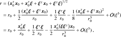 (A.2)
(A.2)
where in the last equality we used the general properties of scalar products, v⊺ w= w⊺v and  . Taking now the expectation of Eq. (A.2) gives
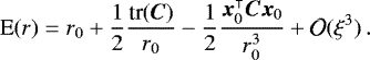 (A.3)
(A.3)
In contrast to Eq. (A.1), the truncated expression in Eq. (A.3) is only approximate, and moreover depends on the unknown quantities r0 and x0. A useful correction for the bias may nevertheless be computed by inserting the estimated quantities r and x for r0 and x0 ; thus
 (A.4)
(A.4)
We can assume that this formula may be useful as long as the bias correction is small in comparison with r.
Equation (A.4) can be made more explicit in terms of the Cartesian components. In the three-dimensional case of interest here we have
![Mathematical equation: \begin{equation*}\begin{split} r_0 \simeq&\, r -\frac{r^2-x^2}{r^3}\frac{\sigma^2_x}{2}+\frac{r^2-y^2}{r^3}\frac{\sigma^2_y}{2} + \frac{r^2-z^2}{r^3}\frac{\sigma^2_z}{2}\\[3pt] &+\frac{xy}{r^3}C_{xy}-\frac{yz}{r^3}C_{yz}-\frac{zx}{r^3}C_{zx} \,. \end{split} \end{equation*}](/articles/aa/full_html/2021/05/aa39734-20/aa39734-20-eq29.png) (A.5)
(A.5)
In the simplest case of isotropic errors,  and Cxy = Cyz = Czx = 0, this gives
 (A.6)
(A.6)
Interestingly, this correction is approximately 2∕3 of the correction obtained by taking the square root of the unbiased estimate of  :
:  .
.
One can note that all the expressions derived thus far are invariant under a rotation of the reference frame. This is easy to demonstrate since the trace of C is invariant, and the quadratic form x⊺Cx is also invariant when both x and C are expressed in the new frame.
Applied to the results of Table 2, where |g| =5.05 μas yr−1 and the errors are nearly isotropic with σ ≃ 0.35 μas yr−1, we find an estimated bias of about +0.024 μas yr−1. That is, our estimate of the amplitude of the glide is statistically too large by about 0.5%, an amount much smaller than the random uncertainty of the amplitude. Although the bias is small in this case, it is important to draw attention to the potential impact that non-linear transformations can have on the estimates.
It is possible to apply the same mathematical methodology to the estimation of potential biases in the spherical coordinates (α, δ) or (l, b) representing the direction of the vector x. However, this would be a purely academic exercise, for it is not clear what is meant by a bias in estimated angles such as α or δ. We refrain from giving the corresponding formulae, lest they should be used improperly. For one thing, they are not invariant to a rotation of the reference frame, so the ‘corrected’ spherical coordinates in the equatorial and galactic systems give slightly different positions on the sky. What is needed to complement the (unbiased) estimate of the modulus of the vector is an unbiased estimate of its direction, which cannot reasonably depend on the chosen reference frame. We believe that the unbiased direction is most simply given by the unit vector x∕x, expressed inits Cartesian components or spherical coordinates. For a trivariate Gaussian error distribution, this direction has the appealing property that any plane containing the direction bisects the distribution in two equal parts; in other words, there is an equal probability that the true direction is on either side of the plane.
References
- Bachchan, R. K., Hobbs, D., & Lindegren, L. 2016, A&A, 589, A71 [NASA ADS] [CrossRef] [EDP Sciences] [Google Scholar]
- Bailer-Jones, C. A. L., Fouesneau, M., & Andrae, R. 2019, MNRAS, 490,5615 [Google Scholar]
- Ball, R. S. 1908, A treatise on Spherical Astronomy, reprinted 2013 by Cambridge University Press, Cambridge [Google Scholar]
- Bastian, U. 1995, ESA SP, 379, 99 [Google Scholar]
- Bland-Hawthorn, J., & Gerhard, O. 2016, ARA&A, 54, 529 [NASA ADS] [CrossRef] [EDP Sciences] [Google Scholar]
- Chakrabarti, S., Wright, J., Chang, P., et al. 2020, ApJ, 902, L28 [Google Scholar]
- Charlot, P., Jacobs, C. S., Gordon, D., et al. 2020, A&A, 644, A159 [EDP Sciences] [Google Scholar]
- Cioni, M. R. L., van der Marel, R. P., Loup, C., & Habing, H. J. 2000, A&A, 359, 601 [Google Scholar]
- Crowley, C., Kohley, R., Hambly, N. C., et al. 2016, A&A, 595, A6 [NASA ADS] [CrossRef] [EDP Sciences] [Google Scholar]
- De Leo, M., Carrera, R., Noël, N. E. D., et al. 2020, MNRAS, 495, 98 [CrossRef] [Google Scholar]
- Efron, B., & Tibshirani, R. 1994, An Introduction to the Bootstrap, Chapman & Hall/CRC Monographs on Statistics & Applied Probability (New York: Taylor & Francis) [Google Scholar]
- Eilers, A.-C., Hogg, D. W., Rix, H.-W., et al. 2020, ApJ, 900, 186 [CrossRef] [Google Scholar]
- Erkal, D., Belokurov, V., Laporte, C. F. P., et al. 2019, MNRAS, 487, 2685 [Google Scholar]
- ESA 1997, The Hipparcos and Tycho Catalogues (ESA SP-1200) [Google Scholar]
- Eubanks, T. M., Matsakis, D. N., Josties, F. J., et al. 1995, IAU Symp., 166, 283 [Google Scholar]
- Fabricius, C., Luri, X., Arenou, F., et al. 2021, A&A, 649, A5 (Gaia EDR3 SI) [Google Scholar]
- Fanselow, J. L. 1983, Observation Model and parameter partial for the JPL VLBI parameter Estimation Software “MASTERFIT-V1.0”, Tech. rep. [Google Scholar]
- Fardal, M. A., Weinberg, M. D., Babul, A., et al. 2013, MNRAS, 434, 2779 [NASA ADS] [CrossRef] [Google Scholar]
- Ferrarese, L., Côté, P., Cuillandre, J.-C., et al. 2012, ApJS, 200, 4 [Google Scholar]
- Fienga, A., Manche, H., Laskar, J., Gastineau, M., & Verma, A. 2016, Notes Scientifiques et Techniques de l’Institut de Mecanique Celeste, 104 [Google Scholar]
- Fienga, A., Deram, P., Viswanathan, V., et al. 2019, Notes Scientifiques et Techniques de l’Institut de Mecanique Celeste, 109 [Google Scholar]
- Fienga, A., Di Ruscio, A., Bernus, L., et al. 2020, A&A, 640, A6 [CrossRef] [EDP Sciences] [Google Scholar]
- Gaia Collaboration (Katz, D., et al.) 2018a, A&A, 616, A11 [NASA ADS] [CrossRef] [EDP Sciences] [Google Scholar]
- Gaia Collaboration (Mignard, F., et al.) 2018b, A&A, 616, A14 [NASA ADS] [CrossRef] [EDP Sciences] [Google Scholar]
- Gaia Collaboration (Brown, A. G. A., et al.) 2021, A&A, 649, A1 (Gaia EDR3 SI) [NASA ADS] [CrossRef] [EDP Sciences] [Google Scholar]
- Garavito-Camargo, N., Besla, G., Laporte, C. F. P., et al. 2020, ApJ, submitted [arXiv:2010.00816] [Google Scholar]
- Grant, R. 1852, History of Physical Astronomy from the Earliest Ages to the Middle of the 19th Century (Palala Press) [Google Scholar]
- GRAVITY Collaboration (Abuter, R., et al.) 2019, A&A, 625, L10 [NASA ADS] [CrossRef] [EDP Sciences] [Google Scholar]
- Gwinn, C. R., Eubanks, T. M., Pyne, T., Birkinshaw, M., & Matsakis, D. N. 1997, ApJ, 485, 87 [NASA ADS] [CrossRef] [Google Scholar]
- Herschel, J. F. W. 1833, A Treatise on Astronomy (London: Longman), reprinted 2009 by Cambridge University Press, Cambridge [Google Scholar]
- Herschel, J. F. W. 1849, Outlines of Astronomy, reprinted 2010 by Cambridge University Press, Cambridge [Google Scholar]
- Hobbs, D., Høg, E., Mora, A., et al. 2016, ArXiv e-prints, [arXiv:1609.07325] [Google Scholar]
- Hunt, J. A. S., Bub, M. W., Bovy, J., et al. 2019, MNRAS, 490, 1026 [Google Scholar]
- Kardashev, N. S. 1986, Sov. Astron., 30, 501 [Google Scholar]
- Kashibadze, O. G., Karachentsev, I. D., & Karachentseva, V. E. 2020, A&A,635, A135 [CrossRef] [EDP Sciences] [Google Scholar]
- Klioner, S. A. 2003, AJ, 125, 1580 [Google Scholar]
- Klioner, S. A. 2004, Phys. Rev. D, 69, 124001 [NASA ADS] [CrossRef] [Google Scholar]
- Klioner, S. 2013, Relativistic Foundations of Astrometry and Celestial Mechanics, ed. W. Van Altena (Cambridge: Cambridge University Press), 47 [Google Scholar]
- Kopeikin, S. M., & Makarov, V. V. 2006, AJ, 131, 1471 [NASA ADS] [CrossRef] [Google Scholar]
- Kovalevsky, J. 2003, A&A, 404, 743 [NASA ADS] [CrossRef] [EDP Sciences] [Google Scholar]
- Lalande, J. 1792, Traité d’Astronomie (Paris: La Veuve Desaint) [Google Scholar]
- Law, D. R., & Majewski, S. R. 2010, ApJ, 714, 229 [NASA ADS] [CrossRef] [Google Scholar]
- Lindegren, L. 2018, unpublished note [Google Scholar]
- Lindegren, L., Hernández, J., Bombrun, A., et al. 2018, A&A, 616, A2 [NASA ADS] [CrossRef] [EDP Sciences] [Google Scholar]
- Lindegren, L., Klioner, S. A., Hernández, J., et al. 2021a, A&A, 649, A2 (Gaia EDR3 SI) [EDP Sciences] [Google Scholar]
- Lindegren, L., Bastian, U., Biermann, M. 2021b, A&A, 649, A4 (Gaia EDR3 SI) [EDP Sciences] [Google Scholar]
- MacMillan, D. S., Fey, A., Gipson, J. M., et al. 2019, A&A, 630, A93 [NASA ADS] [CrossRef] [EDP Sciences] [Google Scholar]
- Malkin, Z. 2014, Journées 2013 Systèmes de référence spatio-temporels’, ed. N. Capitaine, 44 [Google Scholar]
- McMillan, P. J. 2011, MNRAS, 414, 2446 [NASA ADS] [CrossRef] [Google Scholar]
- McMillan, P. J. 2017, MNRAS, 465, 76 [NASA ADS] [CrossRef] [Google Scholar]
- Mei, S., Blakeslee, J. P., Côté, P., et al. 2007, ApJ, 655, 144 [NASA ADS] [CrossRef] [Google Scholar]
- Mignard, F. 2002, EAS Publ. Ser., 2, 327 [Google Scholar]
- Mignard, F., & Klioner, S. 2012, A&A, 547, A59 [NASA ADS] [CrossRef] [EDP Sciences] [Google Scholar]
- Monari, G., Famaey, B., Siebert, A., et al. 2016, MNRAS, 461, 3835 [NASA ADS] [CrossRef] [Google Scholar]
- Monari, G., Famaey, B., Siebert, A., Wegg, C., & Gerhard, O. 2019, A&A, 626, A41 [NASA ADS] [CrossRef] [EDP Sciences] [Google Scholar]
- Paine, J., Darling, J., Graziani, R., & Courtois, H. M. 2020, ApJ, 890, 146 [Google Scholar]
- Patel, E., Kallivayalil, N., Garavito-Camargo, N., et al. 2020, ApJ, 893, 121 [CrossRef] [Google Scholar]
- Pérez-Villegas, A., Portail, M., Wegg, C., & Gerhard, O. 2017, ApJ, 840, L2 [NASA ADS] [CrossRef] [Google Scholar]
- Perryman, M. A. C., de Boer, K. S., Gilmore, G., et al. 2001, A&A, 369, 339 [NASA ADS] [CrossRef] [EDP Sciences] [Google Scholar]
- Pietrzyński, G., Graczyk, D., Gallenne, A., et al. 2019, Nature, 567, 200 [Google Scholar]
- Planck Collaboration III. 2020, A&A, 641, A3 [NASA ADS] [CrossRef] [EDP Sciences] [Google Scholar]
- Pond, J. 1833, Astronomical Observations made at the Royal Observatory at Greenwich, 18, PI-P19, https://ui.adsabs.harvard.edu/abs/1833RGAO...18P...1P [Google Scholar]
- Portail, M., Gerhard, O., Wegg, C., & Ness, M. 2017, MNRAS, 465, 1621 [NASA ADS] [CrossRef] [Google Scholar]
- Read, J. I., & Erkal, D. 2019, MNRAS, 487, 5799 [NASA ADS] [CrossRef] [Google Scholar]
- Reid, M. J., & Brunthaler, A. 2020, ApJ, 892, 39 [Google Scholar]
- Reid, M. J., Menten, K. M., Brunthaler, A., et al. 2014, ApJ, 783, 130 [Google Scholar]
- Riess, A. G., Fliri, J., & Valls-Gabaud, D. 2012, ApJ, 745, 156 [NASA ADS] [CrossRef] [Google Scholar]
- Schönrich, R., Binney, J., & Dehnen, W. 2010, MNRAS, 403, 1829 [NASA ADS] [CrossRef] [Google Scholar]
- Shu, Y., Koposov, S. E., Evans, N. W., et al. 2019, MNRAS, 489, 4741 [Google Scholar]
- Soffel, M., Klioner, S. A., Petit, G., et al. 2003, AJ, 126, 2687 [NASA ADS] [CrossRef] [Google Scholar]
- Sovers, O. J., & Jacobs, C. S. 1996, Observation model and parameter partials for the JPL VLBI parameter estimation software MODEST, 1996, Jet Propulsion Lab. Report [Google Scholar]
- Sovers, O. J., Fanselow, J. L., & Jacobs, C. S. 1998, Rev. Mod. Phys., 70, 1393 [NASA ADS] [CrossRef] [Google Scholar]
- Titov, O., & Krásná, H. 2018, A&A, 610, A36 [NASA ADS] [CrossRef] [EDP Sciences] [Google Scholar]
- Titov, O., & Lambert, S. 2013, A&A, 559, A95 [NASA ADS] [CrossRef] [EDP Sciences] [Google Scholar]
- Titov, O., Lambert, S. B., & Gontier, A.-M. 2011, A&A, 529, A91 [NASA ADS] [CrossRef] [EDP Sciences] [Google Scholar]
- Tully, R. B., Shaya, E. J., Karachentsev, I. D., et al. 2008, ApJ, 676, 184 [NASA ADS] [CrossRef] [Google Scholar]
- Tully, R. B., Courtois, H., Hoffman, Y., & Pomarède, D. 2014, Nature, 513, 71 [NASA ADS] [CrossRef] [Google Scholar]
- Vasiliev, E., & Belokurov, V. 2020, MNRAS, 497, 4162 [Google Scholar]
- Wegg, C., Gerhard, O., & Portail, M. 2015, MNRAS, 450, 4050 [Google Scholar]
- Xu, M. H., Wang, G. L., & Zhao, M. 2012, A&A, 544, A135 [NASA ADS] [CrossRef] [EDP Sciences] [Google Scholar]
Here, and in the following, the acceleration is expressed as a proper motion through division by c, the speed of light; see Eq. (4). (gx, gy, gz) are the components of the effect in the equatorial coordinates defined by the International Celestial Reference System (ICRS).
To take the Solar System as an illustrative analogue: the bottom of the potential trough is always very close to the centre of the Sun, but the barycentre can be off by more than one solar radius, so that the attraction felt by a Kuiper belt object at, say, 30 au can be off by more than 0.5′.
The effective wavenumber νeff is the mean value of the inverse wavelength λ−1, weighted by the detected photon flux in the Gaia passband G. This quantity is extensively used to model colour-dependent image shifts in the astrometric instrument of Gaia. An approximate relation between νeff and the colour index GBP − GRP is given in Lindegren et al. (2021a). The values νeff = 1.3, 1.6, and 1.9 μm−1 roughly correspond to, respectively, GBP − GRP = 2.4, 0.6, and − 0.5.
The RUWE (Lindegren et al. 2021a) is a measure of the goodness-of-fit of the five- or six-parameter model to the observations of the source. The expected value for a good fit is 1.0. A higher value could indicate that the source is not point-like at the optical resolution of Gaia (≃ 0.1′′), or has a time-variable structure.
For the proper motion of a star it is only the differential (tidal) acceleration between the Solar System and the star that matters.
More precisely, the procedure stops the first time the set of outliers is the same as in an earlier iteration (not necessarily the previous one).
The ‘geocentric’ orbit of Gaia is also defined in the BCRS and represents the difference of the BCRS coordinates of Gaia and those of the geocentre.
All Tables
Principal results of this work: equatorial and galactic components of the estimated acceleration of the Solar System, with uncertainties and correlations.
All Figures
|
Fig. 1 Galactic aberration over 500 Myr for an observer looking towards Galactic north. The curve shows the apparent path of a hypothetical quasar, currently located exactly at the north galactic pole, as seen from the Sun (or solar system barycentre).The points along the path show the apparent positions after 0, 50, 100, …Myr due to the changing velocity of the Sun in its epicyclic orbit around the galactic centre. The point labelled GC is the position of the quasar as seen by an observer at rest with respect to the galactic centre. The point labelled CMB is the position as seen by an observer at rest with respect to the cosmic microwave background. The Sun’s orbit was computed using the potential model by McMillan (2017) (see also Sect. 4), with current velocity components derived from the references in Sect. 4.1. The Sun’s velocity with respect to the CMB is taken from Planck Collaboration III (2020). |
| In the text | |
|
Fig. 2 Proper motion field of QSO-like objects induced by the centripetal galactic acceleration. There is no effect in the directions of the galactic centre and anti-centre, and amaximum in the plane passing through the galactic poles with nodes at 90–270° in galactic longitudes. The plot is in galactic coordinates with the Solar System at the centre of the sphere, and the vector field seen from the exterior of the sphere. Orthographic projection with viewpoint at l = 30°, b = 30° and an arbitrary scale for the vectors. See also an online movie. |
| In the text | |
|
Fig. 3 Distribution of the Gaia-CRF3 sources with five-parameter solutions. The plot shows the density of sources per square degree computed from the source counts per pixel using HEALPix of level 6 (pixel size ≃0.84 deg2). This and following full-sky maps use a Hammer–Aitoff projection in galactic coordinates with l = b = 0 at the centre, north up, and l increasing from right to left. |
| In the text | |
|
Fig. 4 Distribution of the statistical weights of the proper motions of the Gaia-CRF3 sources with five-parameter solutions. Statistical weight is calculated as the sum of
|
| In the text | |
|
Fig. 5 Histograms of some important characteristics of the Gaia-CRF3 sources with five-parameter solutions. From top to bottom: G magnitudes, colours represented by the effective wavenumber νeff (see footnote 3), and the astrometric quality indicator RUWE (see footnote 4). |
| In the text | |
|
Fig. 6 Distributions of the normalised parallaxes ϖ∕σϖ
(upper panel), proper motions in right ascension |
| In the text | |
|
Fig. 7 Equatorial (upper panel) and galactic (lower panel) components of the solar system acceleration for fits with different maximal VSH order lmax (‘alone’ means that the three glide components were fitted with no other VSH terms). The error bars represent ± 1σ uncertainties. |
| In the text | |
|
Fig. 8 Equatorial components of the acceleration and their uncertainties for four intervals of G magnitude: G ≤ 18 mag (29 200 sources), 18 < G ≤ 19 mag (146 614 sources), 19 < G ≤ 20 mag (490 161 sources), and G > 20 mag (549 967 sources). The horizontal colour bands visualise the values and uncertainties (the height corresponds to twice the uncertainty) of the corresponding components computed from the whole data set. |
| In the text | |
|
Fig. 9 Equatorial components of the acceleration and their uncertainties for four intervals of the colour represented by the effective wavenumber νeff used in Gaia DR3 astrometry. The quartiles of the νeff distribution for the sources considered in this study are used as the boundaries of the νeff intervals so that each interval contains about 304 000 sources. The horizontal colour bands visualise the values and uncertainties (the height corresponds to twice the uncertainty) of the corresponding components computed from the whole data set. |
| In the text | |
|
Fig. 10 Visualising the error ellipse of the estimated direction of the acceleration estimate in galactic coordinates. The plot is a density map of the directions from 550 000 bootstrap resampling experiments. The colour scale is logarithmic. |
| In the text | |
Current usage metrics show cumulative count of Article Views (full-text article views including HTML views, PDF and ePub downloads, according to the available data) and Abstracts Views on Vision4Press platform.
Data correspond to usage on the plateform after 2015. The current usage metrics is available 48-96 hours after online publication and is updated daily on week days.
Initial download of the metrics may take a while.