| Issue |
A&A
Volume 649, May 2021
|
|
|---|---|---|
| Article Number | A92 | |
| Number of page(s) | 9 | |
| Section | Galactic structure, stellar clusters and populations | |
| DOI | https://doi.org/10.1051/0004-6361/202039503 | |
| Published online | 18 May 2021 | |
Detectability of continuous gravitational waves from isolated neutron stars in the Milky Way
The population synthesis approach
1
Nicolaus Copernicus Astronomical Center, Polish Academy of Sciences, Bartycka 18, 00-716 Warsaw, Poland
e-mail: This email address is being protected from spambots. You need JavaScript enabled to view it.
2
Astronomical Observatory, University of Warsaw, Al. Ujazdowskie 4, 00-478 Warsaw, Poland
e-mail: This email address is being protected from spambots. You need JavaScript enabled to view it.
Received:
23
September
2020
Accepted:
24
February
2021
Abstract
Aims. We estimate the number of pulsars, detectable as continuous gravitational wave sources with the current and future gravitational-wave detectors, assuming a simple phenomenological model of evolving non-axisymmetry of the rotating neutron star.
Methods. We employed a numerical model of the Galactic neutron star population, with the properties established by comparison with radio observations of isolated Galactic pulsars. We generated an arbitrarily large synthetic population of neutron stars and evolved their period, magnetic field, and position in space. We used a gravitational wave emission model based on exponentially decaying ellipticity (i.e. non-axisymmetry of the star) with no assumption of the origin of a given ellipticity. We calculated the expected signal in a given detector for a one-year observation, and assumed a detection criterion of the signal-to-noise ratio of 11.4, comparable to a targeted continous wave search. We analysed the detectable population separately in each detector: Advanced LIGO, Advanced Virgo, and the planned Einstein Telescope. In the calculation of the expected signal we neglect the frequency change of the signals due to the source’s spindown and the Earth’s motion with respect to the solar barycentre.
Results. With conservative values for the neutron star evolution (a supernova rate of once per 100 years, initial ellipticity ϵ0 ≃ 10−5 with no decay of the ellipticity η = thub ≃ 104 Myr), the expected number of detected neutron stars is 0.15 (based on a simulation of 10 M stars) for the Advanced LIGO detector. A broader study of the parameter space (ϵ0, η) is presented. With the planned sensitivity for the Einstein Telescope, and assuming the same ellipiticity model, the expected detection number is 26.4 pulsars during a one-year observing run.
Key words: stars: neutron / gravitational waves / methods: numerical
© ESO 2021
1. Introduction
The discovery of a double black hole merger (Abbott et al. 2016) and a binary neutron star (NS) merger (Abbott et al. 2017a,b) initiated an era of observable gravitational wave (GW) sources. The first catalogue of transient GW events (Abbott et al. 2019a), created after two observational runs O1 and O2, contains 11 sources and the observational run O3 brought nearly one statistically significant detection candidate per week1 (Abbott et al. 2020). Even so, some sources of the gravitational radiation, in particular the continuous waves from rotating deformed (non-axisymmetric) NSs, elude detection, and we only have upper limits on their intrinsic asymmetry (Aasi et al. 2016; Abbott et al. 2017c, 2019b; Steltner et al. 2021; Dergachev & Papa 2020). The community actively pursues many novel methods of detection (see Jaranowski et al. 1998; Krishnan et al. 2004; Antonucci et al. 2008; Astone et al. 2014, 2010; Miller et al. 2018; Abbott et al. 2009; Piccinni et al. 2018; Dupuis & Woan 2005; Dreissigacker et al. 2018; Caride et al. 2019; Dergachev & Papa 2019; Dreissigacker & Prix 2020). Proposed continuous GW emission models include the r-modes (Lindblom et al. 1998; Bildsten 1998; Owen et al. 1998; Andersson et al. 1999) and a fixed rotating axi-asymmetric anisotropy of the quadrupole moment of inertia (Zimmermann & Szedenits 1979; Bonazzola & Gourgoulhon 1996). In this work we concentrate on the latter case. For a more in-depth review of the current state of GW emission models from NSs, see Andersson et al. (2011), Lasky (2015), Riles (2017), Sieniawska & Bejger (2019).
A general estimate of the detectability of a population of NSs in the gravitational emission regime was previously investigated by Regimbau & de Freitas Pacheco (2000), Palomba (2005), Knispel & Allen (2008), and Woan et al. (2018). We revisit this problem by providing a realistic approach to the properties of the estimated population of isolated NSs (solitary, not in a binary system) in our Galaxy, and by more detailed treatment of the detection of the signal. We limit ourselves to a phenomenological parametrisation of the deformation of a NS to find the general constraints on models without investigating physical details that drive the asymmetry of a star. We aim to estimate the fraction of the Galactic population of NSs that can be detected by the Advanced LIGO (Aasi et al. 2015), the Advanced Virgo (Acernese et al. 2015), and the Einstein Telescope (Punturo et al. 2010; Maggiore et al. 2020). We assume the coherent signal intergration time to be tobs = 1 year. Although this period of time is comparable to the current O3 observation run of the LIGO-Virgo Collaboration, it should be noted that the usable scientific data does not cover the whole period (e.g. due to maintenance, quality assurance). Thus, this estimate is the optimistic upper limit of the possible detection rate.
2. Physical model
As the basis for our studies we use the numerical models developed in our previous work (Cieślar et al. 2020). We simulated a population of 107 isolated NSs2 with properties similar to the observed single radio pulsars in the Galaxy (Manchester et al. 2005)3. In our population synthesis model, we include the evolution of period, period derivative, and magnetic field of each NS and trace its position as it moves in the Galactic potential. The magnetic field decay influences the evolution of rotation period and period derivative assuming the magnetic dipole model. We propagate the stars through the Galactic potential, from their birth places (inside the spiral arms), with inclusion of supernova kicks (Hobbs et al. 2005), to their final positions at the current date, when they are observed.
2.1. Radio luminosity
In our model we simulate two phenomenological radio luminosity models. The first is proportional to the rotational energy of the NS:
 (1)
(1)
The other is a power law
 (2)
(2)
where κi are the parameters of the models4, and Ṗ15 is a period derivative divided by 10−15. Since both models produce a population that is identical to the observed one, choosing one over another does not have any implications for the evolution of NS in the context of this work. Therefore, we use the parameters from the rotational model as it contains fewer parameters.
2.2. Age and size of the simulated population
The maximum age of a simulated NS is tage, max = 50 Myr, while the number of stars is Npop = 107. With an assumption that one NS is born every 100 yr, this means a synthetic population that is 20 times higher in the last 50 Myr period. The factor of 20 was picked due to the technical aspects of the simulation; it provides a significant sample to compute statistics while limiting the simulation time.
The exclusion of NSs older than 50 Myr is dictated by one factor: due to the exponential magnetic decay implemented in the model, the NSs evolve faster in the period–period derivative plane. If we consider their characteristic age τ = P/2Ṗ, our population is comparable to the observed population, and reaches characteristic ages of 10 Gyr. Moreover, this means that older solitary NSs reach a region of period–period derivative plane known as the graveyard (a region of periods longer than 1s) and stay there due to the very low period derivative (Ṗ < 10−22 [s s−1]). This region is outside the frequency range of the current detectors (Advanced LIGO and Advanced Virgo) and of the planned, next-generation observatories (Einstein Telescope).
2.3. Model parameters
The parameters of the model used in this paper are shown in Table 1. The distributions describing the population’s parameters and details of the pulsar evolution model are described in Cieślar et al. (2020). The pulsar population model provides us with a population of NSs, and for each NS we have its position in the sky, distance, rotation period, period derivative, and pulsar age.
Values of the parameters describing the NS evolution model.
2.4. Millisecond pulsars excluded from the model
A standard model for of evolution of millisecond pulsars (MSPs) indicate that they are produced via accretion in low mass X-ray binaries (see Bhattacharya & van den Heuvel 1991), although it should be noted that not all observed MSPs can be confidently described by this model (Kiziltan & Thorsett 2009). Modelling a standard MSP with an accretion phase requires a very detailed treatment of the binary interactions (e.g. Belczynski et al. 2008). This treatment of binary interactions is beyond the scope of the NS evolution model presented in our previous work (Cieślar et al. 2020), thus we limit this work to probing solitary NSs.
2.5. Gravitational wave signal from a rotating ellipsoid
The GW signal registered in the detector is given by the dimensionless amplitude
 (3)
(3)
where F+ and F× denote the antenna pattern functions (see Sect. 2.5.2 for details). Since the two wave polarisations (+ and ×) are orthogonal, the measured quantity is the root of the square of h:
 (4)
(4)
We assume a general model of a rotating triaxial ellipsoid after Bonazzola & Gourgoulhon (1996). We do not assume the cause of the deformation, but merely state that it is necessary for the time-varying quadruple moment of the NS mass (for different theoretical models of NS deformation see Ostriker & Gunn 1969; Melosh 1969; Chau 1970; Press & Thorne 1972). The ellipticity of the NS is defined as
 (5)
(5)
where I is the mean NS moment of inertia with respect to the rotational axis, and I1 and I2 are moments in the plane perpendicular to the principal axis. The amplitudes of the GW in both polarisations can be written as
 (6)
(6)
where  ,
,  ,
,  , and D = sin χ cos ι. The NS signal is parametrised by the angle between the rotation axis and the major axis of the elipticity χ, the line of sight inclination ι, the rotational period P, the time t, and the time corresponding to a phase-shift t0. The amplitude h0 is defined as
 (7)
(7)
where G is the gravitational constant, c is the speed of light, and r is the distance to the star.
2.5.1. Average emission over the NS period
Because the parameters A, B, C, and D are independent of the time, we compute an average of h2 over the period P = 1/ν, where ν is the frequency:
 (8)
(8)
The term ⟨h2⟩P represents the average power of emitted GW signal at two harmonics:  and
and  . In our analysis we emulate the simplest approach of detecting a NS at a single frequency with its amplitude above a certain level (see Sect. 2.6). Therefore, we treat the amplitude of the GW in each frequency independently:
 (9)
(9)
2.5.2. Antenna pattern and sidereal day average
The detectors are described by four parameters. Their geographical position longitude and latitude, the angle between their arms, and the angle measured anticlockwise between the east and the bisector of the arms. The NS location in the sky is described by the equatorial coordinates: the right ascension, the declination, and the polarisation angle (the orientation of the rotation axis with respect to the line of sight). We follow the work of Jaranowski et al. (1998, see Eqs. (10)–(13) therein) with the antenna power in + and × wave polarisations. We average the antenna pattern over one full rotation of the Earth, yielding a final average (over the NS period and a sidereal day). The square of registered GW amplitude is
 (10)
(10)
Similar to Eq. (9), we divide the period-average and day-average into two separate harmonics:
 (11)
(11)
2.6. Detector sensitivity and signal integration
For the Advanced LIGO and Advanced Virgo detectors, we assume the amplitude spectral density of the noise  (expressed in units of strain/
 ) from the first three-months of the O3 observation run5 to be representative and constant for the whole period of our analysis (Abbott et al. 2018, living review, see arXiv version for the latest update). We also analyse the future Einstein Telescope in the D configuration (ET-D; three detection arm pairs in the shape of an equilateral triangle, see Hild et al. 2011). The location of this facility has not been chosen yet. In that regard, we assume the same location for ET-D as for the Advanced Virgo detector. We scale the sensitivity6 appropriately for the D configuration by a factor
  (see Hild et al. 2011). Also, we sum the signal from its three arms (E1, E2, E3) as
  .
.
Since the signal from a NS comes at two harmonics (ν and 2ν, see Eq. (9)), we define the signal-to-noise ratio (S/N; see Jaranowski & Krolak 2009, Ch. 7) separately for each harmonic,
 (12)
(12)
where tobs is the integration time. The tobs is far greater then period P or a sidereal day D over which the signal from the NS is averaged (see Eq. (11)). We assume a detection threshold for a pulsar of S/Nν, 2ν = 11.4 (after Abbott et al. 2004) because our simulation resembles a single-template search of a known pulsar; we assume that we know the position in the sky and neglect the error associated with it and we compare the signal with a corresponding frequency bin in the detector noise. We simulate the integration time of one year tobs = 31 536 000 s. Thus, we use the detectability threshold
 (13)
(13)
and state that a NS is detected in a given harmonic (either ν or 2ν) if the averaged, detected strain crosses the threshold:
 (14)
(14)
2.7. Neutron star asymmetry model
A NS must be asymmetric with respect to the rotation axis to emit GWs. There are many models that predict some level of asymmetry. In this work we do not want to concentrate on any particular physical model. Instead, we propose a simple two-parameter phenomenological model of evolution of a NS asymmetry. We assume that there is an initial asymmetry ϵ0 at the time the NS is formed, and that it decays on a timescale of η. Thus, at a given moment of time the asymmetry is given by
 (15)
(15)
With such a model we can explore the general parameter space of possible mechanisms of asymmetry generation, and place observational constraints on such a space.
3. Results and discussion
We now proceed to the estimation of the detectability of the GWs from NSs. We use the standard model of properties of the NS population (Cieślar et al. 2020), and for each NS we calculate the expected S/N of the GW given its actual position in the sky, distance, period, and ellipticity. For each model of evolution of ellipticity characterised by two parameters ϵ0 and η we calculate the expected number of observed NSs. We normalise our results to a population where a NS is formed in the Milky Way every 100 years; however, we estimate the population for a much larger model population (10 M stars, 1 every 5 yr). Thus, after normalisation we can obtain the expected number of observed NSs below unity.
We present the results for the Advanced LIGO Livingston in Figs. 1a and b, and for the Advanced Virgo detector in Figs. 2a and b respectively for the ν and 2ν harmonics of the signal (see Eq. (9)). The colours in these figures correspond to the number of detectable NSs in the entire sky for each model as a function of the parameters ϵ0 and η. The dark dashed line in each plot corresponds to the models with the expected one detection; we expect less than one detection in the region of parameter space below this line. A very low number of stars crossing the detection criteria in some regions of the plots may induce arbitrary shapes due to a too low static (most prominently seen in Figs. 2c and d). We disregard such shapes because a significant increase in simulated stars would be needed to smooth the low-detection region in Figs. 1 and 2. The detectability of the pulsar population with the Advanced detectors, where the noise level is a factor two lower (below 200 Hz) then the current level, could improve the detectability by a factor of 3 for the H1 detector and by a factor of 7 for the L1 detector. However, this increase would remain below that of a single detected NS.
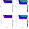 |
Fig. 1. Number of observable pulsars in one-year observations in the space of the parameters of the model η − ϵ0 for the Advanced LIGO detectors. The left column corresponds to the signal’s ν harmonic, the right column the 2ν harmonic. The colour represents the expected number of detections for each model. The black dashed line in each plot corresponds to the models where one pulsar detection is expected. All models below the black dashed line correspond to less than one expected detection. The blue vertical dashed line indicates models where η is equal to the magnetic field decay Δ (see Table 1). (a) ν. L1 Advanced LIGO detector at Livingston. (b) 2ν. L1 Advanced LIGO detector at Livingston. (c) ν. H1 Advanced LIGO detector at Hanford. (d) 2ν. H1 Advanced LIGO detector at Hanford. |
 |
Fig. 2. Number of observable pulsars in one-year observations in the space of the parameters of the model η − ϵ0 for the Advanced Virgo and Einstein Telescope detectors. The left column corresponds to the signal’s ν harmonic, the right column the 2ν harmonic. The black dashed line in each plot corresponds to the models where one pulsar detection is expected. All models below the black dashed line correspond to less than one expected detection. The blue vertical dashed line indicates models where η is equal to the magnetic field decay Δ (see Table 1). (a) ν. V1 Advanced Virgo detector. (b) 2ν. V1 Advanced Virgo detector. (c) ν. ET-D Einstein Telescope detector, configuration D. (d) 2ν. ET-D Einstein Telescope detector, configuration D. |
For the models where the population evolves slowly (i.e. η > 0.1 Myr), we expect at least one detection for the 2ν harmonic with the Advanced LIGO detectors assuming the initial ellipticity ϵ0 > 2.5 × 10⁻⁵ and ϵ0 > 6.3 × 10⁻⁵ for the Advanced Virgo detector. For the population of quickly evolving ellipticity the detectability quickly becomes more difficult as the timescale η decreases. This is due to the fact that the number of NSs with sufficiently large ellipiticity in the Milky Way at a given time becomes smaller.
The similar diagrams calculated for the sensitivity of ET are shown in Figs. 2c and d. For this detector in the regime of slowly varying ellipticity (i.e. with η > 0.1 Myr) the detectable models have the initial ellipticity ϵ0 > 7.9 × 10⁻⁷ for the 2ν harmonic, and ϵ0 > 5.6 × 10⁻⁶ for the ν harmonic. The population becomes undetectable for η < 100 yr as in this case the ellipticity decreases on a timescale comparable to the time between consecutive supernova explosions in the Galaxy.
It is quite interesting to investigate in more detail the properties of the detectable population. In Fig. 3 we present the maximum age of pulsars in the detectable population as a function of the model parameters η and ϵ0 for the case of Advanced Virgo and the Einstein Telescope. For detectable NSs in all models, for the current Advanced detectors, the maximum age is not greater than 1 Myr because only the youngest NSs crossed the threshold of the detection.
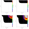 |
Fig. 3. Maximum age of visible NSs in one-year observations in the space of the parameters of the model η − ϵ0 for the Advanced Virgo and Einstein Telescope detectors. The left column corresponds to the signal’s ν harmonic, the right column the 2ν harmonic. The colour represents the maximum age in the population for a given model. The blue vertical dashed line indicates models where η is equal to the magnetic field decay Δ (see Table 1). (a) ν. V1 Advanced Virgo detector. (b) 2ν. V1 Advanced Virgo detector. (c) ν. Einstein Telescope detector, configuration D. (d) 2ν. Einstein Telescope detector, configuration D. |
We now concentrate on a single model with a 2.3 and 26.4 detections, for the ν and 2ν harmonics respectively, in the Einstein Telescope described by ϵ0 = 10−5 and η = 104 Myr (see Table 2). In Figs. 4 and 5 we present the population of NSs on a diagram spanned by the GW frequency and the mean value of the GW amplitude. We also plot the detection threshold curves corresponding to one-year integration and a S/N threshold of 11.4 for the current detectors and for ET-D. We note that the detectable populations will change by a factors ranging from 3 for the H1 detector to 7 for the L1 detector if the threshold is lowered to S/N = 5. In comparison, ET-D will increase its number of visible NSs only by a factor of 3. The discrepancy is due to the very poor statistics of the easiest-to-detect NSs, which leads to the conclusion that a factor of 7 may be an overestimate. The density of the population of NSs is shown as a colour map. The observable NSs have frequencies in the range of approximately 10−300 Hz, with rare NSs going above 300 Hz, when searching for the signal’s 2ν harmonic (see Fig. 6), and correspondingly lower for the signal’s ν harmonic. In Fig. 7 we compare the detectable GW population (the colour represents the amplitude of the signal’s 2ν harmonic) with the population of single pulsars in the Galaxy (based on the Australia Telescope National Facility Pulsar Catalogue, Manchester et al. 2005). The population of NSs that can be detected in ET-D lies mostly in the upper left corner of the period–period derivative plane, which corresponds to very young NSs. Since NSs are born in the Galactic disk, this leads to a spatially concentrated distribution (see Fig. 8).
Expected number of detection for a model with parameters equal to ϵ0 = 10−5 and η = 104 Myr.
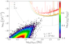 |
Fig. 4. Sensitivity curves for the detectors of Advanced LIGO (L1, H1), Advanced Virgo (V1), and the Einstein Telescope in configuration D for the signal’s ν harmonic of the population of NSs. The model parameters are ϵ0 = 10−5, and η = 104 Myr. The sensitivity of the detectors is scaled by one year of integration time ( |

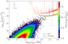 |
Fig. 5. Sensitivity curves for the detectors of Advanced LIGO (L1, H1), Advanced Virgo (V1), and the Einstein Telescope in configuration D for the signal’s 2ν harmonic of the population of NSs. The model parameters are ϵ0 = 10−5, and η = 104 Myr. The sensitivity of the detectors is scaled by one year of integration time ( |

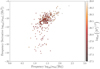 |
Fig. 6. Frequency–frequency derivative plane. The colour represents the emitted GW at 2ν frequency for the Einstein Telescope in configuration D for one year of integration time. The model parameters are ϵ0 = 10−5, η = 104. The presented population is 20 times larger than the expected Galactic population. |
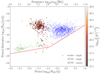 |
Fig. 7. Period–period derivative plane. The colour represents the emitted GW at 2ν frequency for the Einstein Telescope in configuration D for one year of integration time. The model parameters are ϵ0 = 10−5, η = 104. The presented population is 20 times larger than the expected Galactic population. The blue dots represent the population of observed single pulsars. The green dots represent the population of observed pulsars in binary systems (MSPs). The observed populations are from the Australia Telescope National Facility (ATNF) Pulsar Catalogue (Manchester et al. 2005). The red lines represent the death lines, i.e. the theoretical limits for effective radio emission (Rudak & Ritter 1994). |
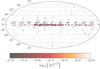 |
Fig. 8. Spatial distribution in the Galactic coordinates of the visible population in the Einstein Telescope configuration D, at the 2ν frequency. The model parameters are ϵ0 = 10−5, η = 104. |
In Fig. 6 we present the population of pulsars detectable in ET in the space of variables used in gravitational wave searches: frequency and frequency derivative. The typical values of the frequency derivative  are in the range from 10−18 Hz2 to 10−8 Hz2. Thus, most of the potentially detectable pulsars have a frequency derivative that is not detectable. The frequencies of the detectable pulsars all lie below 300 Hz, and the bulk of the detectable objects have frequencies in the range from 10 Hz to 60 Hz.
As a result the optimal strategy to look for GW from isolated rotating NSs concentrates on the surveys of the Galactic disk. In the case of the Advanced detectors we expect detected pulsars only at 2ν harmonic with frequencies in the range 30−300 Hz. In the case of the ET the bulk of detections will be in the frequency range from 20 to 100 Hz for the ν harmonic and 10 to 100 Hz for the 2ν harmonic. The frequency derivatives of the brightest systems are above 10−8 Hz2, while the typical values of the frequency derivative in the population detectable by the ET is from 10−12 to 10−9 Hz2. The largest value of the frequency derivative in the recent search by Abbott et al. (2019b) was only 10−8 Hz2. Narrowing down the parameter space for the searches as suggested above will increase the chances of detection.
If we inspect all detected pulsars (green and blue populations in Fig. 7) we note that the MSPs (green population) reside mostly in the frequency range from 200 Hz to 2 kHz for the more prominent harmonic of fGW = 2fNS. Their addition could improve the detection prospects. However, answering questions about quantitative improvement would require addressing the binary interactions (see Sect. 2.4), and would also require a more detailed model of the asymmetry that treats the initial and accretion induced inhomogeneity of the NS momentum.
4. Conclusions
We presented our estimation of the detectability of the Galactic population of isolated NSs. With a high value of the initial ellipticity (ϵ0 ≃ 10−5) and no decay in the moment of inertia non-uniformity (decay scale η = thub ≃ 104 Myr), the expected number of detected NSs in the Advanced detectors is still less then 1. Since the increase in S/N is proportional to square root of time (S/N ∼  ), we do not expect a drastic change in the estimates for the Advanced LIGO and Advanced Virgo detectors. The most limiting factor is the low frequency sensitivity (below 100 Hz) of the detectors. As shown in Fig. 2c, we expect that future experiments such as the Einstein Telescope will clearly improve the prospect of continuous GW signal discovery.
We present the parameter space of the most likely discovery of solitary pulsars: the range frequencies, frequency derivatives, and position in the sky. We suggest that narrowing down searches in this restricted parameter space may increase the effective sensitivity and increase the chance of detection.
107 NSs is roughly 20 times more than an expected Galactical population. This number represents a trade-off between statistical error and computational speed.
Symbols describing the parameters of the luminosity models were simplified with respect to our previous work (Cieślar et al. 2020).
For the sensitivity curves see https://dcc.ligo.org/LIGO-T2000012/public
For the sensitivity curve see https://tds.virgo-gw.eu/?content=3r=14065
Acknowledgments
We would like to thank Brynmore Haskell and Graham Woan for comments and fruitful discussion. MC and TB are supported by the grant “AstroCeNT: Particle Astrophysics Science and Technology Centre” (MAB/2018/7) carried out within the International Research Agendas programme of the Foundation for Polish Science (FNP) financed by the European Union under the European Regional Development Fund. Part of this work was supported by Polish National Science Centre (NCN) grants no. 2016/22/E/ST9/00037 and 2017/26/M/ST9/00978. TB, MS, and NS acknowledge support of the TEAM/2016-3/19 grant from FNP. MS was partially supported by the NCN grant no. 2018/28/T/ST9/00458.
References
- Aasi, J., Abbott, B. P., Abbott, R., et al. 2015, Class. Quant. Grav., 32, 074001 [CrossRef] [Google Scholar]
- Aasi, J., Abbott, B. P., Abbott, R., et al. 2016, Phys. Rev. D, 93, 042007 [Google Scholar]
- Abbott, B., Abbott, R., Adhikari, R., et al. 2004, Phys. Rev. D, 69, 082004 [NASA ADS] [CrossRef] [Google Scholar]
- Abbott, B., Abbott, R., Adhikari, R., et al. 2009, Phys. Rev. D, 79, 022001 [Google Scholar]
- Abbott, B. P., Abbott, R., Abbott, T. D., et al. 2016, Phys. Rev. Lett., 116, 061102 [Google Scholar]
- Abbott, B. P., Abbott, R., Abbott, T. D., et al. 2017a, Phys. Rev. Lett., 119, 161101 [Google Scholar]
- Abbott, B. P., Abbott, R., Abbott, T. D., et al. 2017b, ApJ, 848, L12 [Google Scholar]
- Abbott, B. P., Abbott, R., Abbott, T. D., et al. 2017c, Phys. Rev. D, 96, 122004 [Google Scholar]
- Abbott, B. P., Abbott, R., Abbott, T. D., et al. 2018, Liv. Rev. Relativ., 21, 3 [Google Scholar]
- Abbott, B. P., Abbott, R., Abbott, T. D., et al. 2019a, Phys. Rev. X, 9, 031040 [Google Scholar]
- Abbott, B. P., Abbott, R., Abbott, T. D., et al. 2019b, Phys. Rev. D, 100, 024004 [Google Scholar]
- Abbott, R., Abbott, T. D., Abraham, S., et al. 2020, ArXiv e-prints [arXiv:2010.14527] [Google Scholar]
- Acernese, F., Agathos, M., Agatsuma, K., et al. 2015, Class. Quant. Grav., 32, 024001 [Google Scholar]
- Andersson, N., Kokkotas, K. D., & Stergioulas, N. 1999, ApJ, 516, 307 [NASA ADS] [CrossRef] [Google Scholar]
- Andersson, N., Ferrari, V., Jones, D. I., et al. 2011, Gen. Rel. Grav., 43, 409 [Google Scholar]
- Antonucci, F., Astone, P., Antonio, S. D., Frasca, S., & Palomba, C. 2008, Class. Quant. Grav., 25, 184015 [Google Scholar]
- Astone, P., D’Antonio, S., Frasca, S., & Palomba, C. 2010, Class. Quant. Grav., 27, 194016 [Google Scholar]
- Astone, P., Colla, A., D’Antonio, S., Frasca, S., & Palomba, C. 2014, Phys. Rev. D, 90, 042002 [Google Scholar]
- Belczynski, K., Kalogera, V., Rasio, F. A., et al. 2008, ApJS, 174, 223 [NASA ADS] [CrossRef] [Google Scholar]
- Bhattacharya, D., & van den Heuvel, E. P. J. 1991, Phys. Rep., 203, 1 [NASA ADS] [CrossRef] [Google Scholar]
- Bildsten, L. 1998, ApJ, 501, L89 [NASA ADS] [CrossRef] [Google Scholar]
- Bonazzola, S., & Gourgoulhon, E. 1996, A&A, 312, 675 [NASA ADS] [Google Scholar]
- Caride, S., Inta, R., Owen, B. J., & Rajbhandari, B. 2019, Phys. Rev. D, 100, 064013 [Google Scholar]
- Chau, W. Y. 1970, Nature, 228, 655 [Google Scholar]
- Cieślar, M., Bulik, T., & Osłowski, S. 2020, MNRAS, 492, 4043 [Google Scholar]
- Dergachev, V., & Papa, M. A. 2019, Phys. Rev. Lett., 123, 101101 [Google Scholar]
- Dergachev, V., & Papa, M. A. 2020, Phys. Rev. Lett., 125, 171101 [Google Scholar]
- Dreissigacker, C., & Prix, R. 2020, Phys. Rev. D, 102, 022005 [Google Scholar]
- Dreissigacker, C., Prix, R., & Wette, K. 2018, Phys. Rev. D, 98, 084058 [Google Scholar]
- Dupuis, R. J., & Woan, G. 2005, Phys. Rev. D, 72, 102002 [Google Scholar]
- Hild, S., Abernathy, M., Acernese, F., et al. 2011, Class. Quant. Grav., 28, 094013 [NASA ADS] [CrossRef] [Google Scholar]
- Hobbs, G., Lorimer, D. R., Lyne, A. G., & Kramer, M. 2005, MNRAS, 360, 974 [NASA ADS] [CrossRef] [Google Scholar]
- Jaranowski, P., & Krolak, A. 2009, Analysis of Gravitational-Wave Data (Cambridge: Cambridge University Press) [Google Scholar]
- Jaranowski, P., Królak, A., & Schutz, B. F. 1998, Phys. Rev. D, 58, 063001 [Google Scholar]
- Kiziltan, B., & Thorsett, S. E. 2009, ApJ, 693, L109 [NASA ADS] [CrossRef] [Google Scholar]
- Knispel, B., & Allen, B. 2008, Phys. Rev. D, 78, 044031 [Google Scholar]
- Krishnan, B., Sintes, A. M., Papa, M. A., et al. 2004, Phys. Rev. D, 70, 082001 [Google Scholar]
- Lasky, P. D. 2015, PASA, 32, e034 [CrossRef] [Google Scholar]
- Lindblom, L., Owen, B. J., & Morsink, S. M. 1998, Phys. Rev. Lett., 80, 4843 [NASA ADS] [CrossRef] [Google Scholar]
- Maggiore, M., Broeck, C. V. D., Bartolo, N., et al. 2020, JCAP, 2020, 050 [CrossRef] [Google Scholar]
- Manchester, R. N., Hobbs, G. B., Teoh, A., & Hobbs, M. 2005, AJ, 129, 1993 [NASA ADS] [CrossRef] [Google Scholar]
- Melosh, H. J. 1969, Nature, 224, 781 [Google Scholar]
- Miller, A., Astone, P., D’Antonio, S., et al. 2018, Phys. Rev. D, 98, 102004 [Google Scholar]
- Ostriker, J. P., & Gunn, J. E. 1969, ApJ, 157, 1395 [NASA ADS] [CrossRef] [Google Scholar]
- Owen, B. J., Lindblom, L., Cutler, C., et al. 1998, Phys. Rev. D, 58, 084020 [NASA ADS] [CrossRef] [Google Scholar]
- Palomba, C. 2005, MNRAS, 359, 1150 [NASA ADS] [CrossRef] [Google Scholar]
- Piccinni, O. J., Astone, P., D’Antonio, S., et al. 2018, Class. Quant. Grav., 36, 015008 [Google Scholar]
- Press, W. H., & Thorne, K. S. 1972, ARA&A, 10, 335 [NASA ADS] [CrossRef] [Google Scholar]
- Punturo, M., Abernathy, M., Acernese, F., et al. 2010, Class. Quant. Grav., 27, 194002 [Google Scholar]
- Regimbau, T., & de Freitas Pacheco, J. A. 2000, A&A, 359, 242 [NASA ADS] [Google Scholar]
- Riles, K. 2017, Mod. Phys. Lett. A, 32, 1730035 [Google Scholar]
- Rudak, B., & Ritter, H. 1994, MNRAS, 267, 513 [Google Scholar]
- Sieniawska, M., & Bejger, M. 2019, Universe, 5, 217 [Google Scholar]
- Steltner, B., Papa, M. A., Eggenstein, H. B., et al. 2021, ApJ, 909, 79 [Google Scholar]
- Woan, G., Pitkin, M. D., Haskell, B., Jones, D. I., & Lasky, P. D. 2018, ApJ, 863, L40 [NASA ADS] [CrossRef] [Google Scholar]
- Zimmermann, M., & Szedenits, E. 1979, Phys. Rev. D, 20, 351 [NASA ADS] [CrossRef] [Google Scholar]
All Tables
Expected number of detection for a model with parameters equal to ϵ0 = 10−5 and η = 104 Myr.
All Figures
|
Fig. 1. Number of observable pulsars in one-year observations in the space of the parameters of the model η − ϵ0 for the Advanced LIGO detectors. The left column corresponds to the signal’s ν harmonic, the right column the 2ν harmonic. The colour represents the expected number of detections for each model. The black dashed line in each plot corresponds to the models where one pulsar detection is expected. All models below the black dashed line correspond to less than one expected detection. The blue vertical dashed line indicates models where η is equal to the magnetic field decay Δ (see Table 1). (a) ν. L1 Advanced LIGO detector at Livingston. (b) 2ν. L1 Advanced LIGO detector at Livingston. (c) ν. H1 Advanced LIGO detector at Hanford. (d) 2ν. H1 Advanced LIGO detector at Hanford. |
| In the text | |
|
Fig. 2. Number of observable pulsars in one-year observations in the space of the parameters of the model η − ϵ0 for the Advanced Virgo and Einstein Telescope detectors. The left column corresponds to the signal’s ν harmonic, the right column the 2ν harmonic. The black dashed line in each plot corresponds to the models where one pulsar detection is expected. All models below the black dashed line correspond to less than one expected detection. The blue vertical dashed line indicates models where η is equal to the magnetic field decay Δ (see Table 1). (a) ν. V1 Advanced Virgo detector. (b) 2ν. V1 Advanced Virgo detector. (c) ν. ET-D Einstein Telescope detector, configuration D. (d) 2ν. ET-D Einstein Telescope detector, configuration D. |
| In the text | |
|
Fig. 3. Maximum age of visible NSs in one-year observations in the space of the parameters of the model η − ϵ0 for the Advanced Virgo and Einstein Telescope detectors. The left column corresponds to the signal’s ν harmonic, the right column the 2ν harmonic. The colour represents the maximum age in the population for a given model. The blue vertical dashed line indicates models where η is equal to the magnetic field decay Δ (see Table 1). (a) ν. V1 Advanced Virgo detector. (b) 2ν. V1 Advanced Virgo detector. (c) ν. Einstein Telescope detector, configuration D. (d) 2ν. Einstein Telescope detector, configuration D. |
| In the text | |
|
Fig. 4. Sensitivity curves for the detectors of Advanced LIGO (L1, H1), Advanced Virgo (V1), and the Einstein Telescope in configuration D for the signal’s ν harmonic of the population of NSs. The model parameters are ϵ0 = 10−5, and η = 104 Myr. The sensitivity of the detectors is scaled by one year of integration time ( |
| In the text | |
|
Fig. 5. Sensitivity curves for the detectors of Advanced LIGO (L1, H1), Advanced Virgo (V1), and the Einstein Telescope in configuration D for the signal’s 2ν harmonic of the population of NSs. The model parameters are ϵ0 = 10−5, and η = 104 Myr. The sensitivity of the detectors is scaled by one year of integration time ( |
| In the text | |
|
Fig. 6. Frequency–frequency derivative plane. The colour represents the emitted GW at 2ν frequency for the Einstein Telescope in configuration D for one year of integration time. The model parameters are ϵ0 = 10−5, η = 104. The presented population is 20 times larger than the expected Galactic population. |
| In the text | |
|
Fig. 7. Period–period derivative plane. The colour represents the emitted GW at 2ν frequency for the Einstein Telescope in configuration D for one year of integration time. The model parameters are ϵ0 = 10−5, η = 104. The presented population is 20 times larger than the expected Galactic population. The blue dots represent the population of observed single pulsars. The green dots represent the population of observed pulsars in binary systems (MSPs). The observed populations are from the Australia Telescope National Facility (ATNF) Pulsar Catalogue (Manchester et al. 2005). The red lines represent the death lines, i.e. the theoretical limits for effective radio emission (Rudak & Ritter 1994). |
| In the text | |
|
Fig. 8. Spatial distribution in the Galactic coordinates of the visible population in the Einstein Telescope configuration D, at the 2ν frequency. The model parameters are ϵ0 = 10−5, η = 104. |
| In the text | |
Current usage metrics show cumulative count of Article Views (full-text article views including HTML views, PDF and ePub downloads, according to the available data) and Abstracts Views on Vision4Press platform.
Data correspond to usage on the plateform after 2015. The current usage metrics is available 48-96 hours after online publication and is updated daily on week days.
Initial download of the metrics may take a while.