| Issue |
A&A
Volume 649, May 2021
|
|
|---|---|---|
| Article Number | A71 | |
| Number of page(s) | 13 | |
| Section | Astrophysical processes | |
| DOI | https://doi.org/10.1051/0004-6361/202039278 | |
| Published online | 13 May 2021 | |
Relativistic fluid modelling of gamma-ray binaries
II. Application to LS 5039
Institut für Astro- und Teilchenphysik, Leopold-Franzens-Universität Innsbruck, 6020 Innsbruck, Austria
e-mail: david.huber@uibk.ac.at
Received:
26
August
2020
Accepted:
28
February
2021
Context. In the first paper of this series, we presented a numerical model for the non-thermal emission of gamma-ray binaries in a pulsar-wind-driven scenario.
Aims. We apply this model to one of the best-observed gamma-ray binaries, the LS 5039 system.
Methods. The model involves a joint simulation of the interaction between the pulsar wind and the stellar wind and the transport of electron pairs from the pulsar wind accelerated at the emerging shock structure. We compute the synchrotron and inverse Compton emission in a post-processing step while consistently accounting for relativistic beaming and γγ-absorption in the stellar radiation field.
Results. The wind interaction leads to the formation of an extended, asymmetric wind collision region that develops strong shocks, turbulent mixing, and secondary shocks in the turbulent flow. Both the structure of the collision region and the resulting particle distributions show significant orbital variation. In addition to the acceleration of particles at the bow-like pulsar wind and the Coriolis shock, the model naturally accounts for the re-acceleration of particles at secondary shocks that contribute to the emission at very-high-energy (VHE) gamma-rays. The model successfully reproduces the main spectral features of LS 5039. While the predicted light curves in the high-energy and VHE gamma-ray band are in good agreement with observations, our model still does not reproduce the X-ray to low-energy gamma-ray modulation, which we attribute to the employed magnetic field model.
Conclusions. We successfully model the main spectral features of the observed multi-band, non-thermal emission of LS 5039 and thus further substantiate a wind-driven interpretation of gamma ray binaries. Open issues relate to the synchrotron modulation, which might be addressed through a magnetohydrodynamic extension of our model.
Key words: radiation mechanisms: non-thermal / gamma rays: stars / methods: numerical / relativistic processes / hydrodynamics / stars: individual: LS 5039
© ESO 2021
1. Introduction
Gamma-ray binaries are composed of an early-type, massive star in orbit with a compact object, either a neutron star or a black hole, and are distinguished from X-ray binaries by a dominant radiative output in the gamma-ray regime > 1 MeV (see Dubus 2013; Paredes & Bordas 2019, for a review). They exhibit broadband non-thermal emission, which is modulated with the orbital phase for most systems.
In the literature, two possible mechanisms are proposed to explain their non-thermal emission (see e.g., Mirabel 2006; Romero et al. 2007): a microquasar scenario, where high-energy particles are produced in relativistic jets powered by the accretion of stellar matter onto the compact object (see e.g., Bosch-Ramon & Khangulyan 2009); or a wind-driven scenario, where the compact object is commonly assumed to be a pulsar, accelerating particles at the shocks formed in the wind collision region (WCR) through the interaction between the stellar wind and the relativistic pulsar wind (see Maraschi & Treves 1981; Dubus 2006).
In this work, we will specifically focus on the LS 5039 system, one of the most closely studied gamma-ray binaries, which constitutes a suitable test bed for different modelling approaches thanks to well-known orbital parameters and a wealth of available broadband data. The LS 5039 system is composed of a massive O-type star in a mildly eccentric (e = 0.35) ∼3.9 d orbit with a compact object (Casares et al. 2005). This system is widely assumed to be a representative of the wind-driven scenario, where the compact object is assumed to be a pulsar, which is supported by the available data that show regular orbital modulations in X-rays (Takahashi et al. 2009) as well as low-energy (LE; Collmar & Zhang 2014), high-energy (HE; Abdo et al. 2009), and very-high-energy (VHE; Aharonian et al. 2005) gamma-rays.
The system shows correlated orbital modulations in the X-ray, LE, and VHE bands, peaking at inferior conjunction (when the compact object passes in front of the star as seen by the observer) and reaching its minimum close to superior conjunction (the compact object passes behind the star). In contrast, the HE modulation is anti-correlated with the previously mentioned bands, peaking at superior conjunction.
Most emission models for LS 5039 are purely leptonic, establishing synchrotron emission and anisotropic inverse Compton scattering on the stellar radiation field as the dominant radiative processes (see e.g., Zabalza et al. 2013; Dubus et al. 2015; Molina & Bosch-Ramon 2020). While inverse Compton scattering is most efficient at superior conjunction, where the stellar photons are back-scattered in the direction of the observer (see e.g., Dubus et al. 2008), the attenuation of the VHE flux due to the γγ pair-production process (see e.g., Dubus 2006) is also at its highest there since the generated radiation has to propagate through the binary system before it can escape. Since the shocked pulsar wind retains relativistic velocities (see e.g., Bogovalov et al. 2008), the emission reaching the observer at Earth is modulated by relativistic boosting (see e.g., Dubus et al. 2010) that depends on the orientation of the system. This interplay between the generation of inverse Compton emission and its absorption by pair production together with the phase-dependent relativistic boosting is commonly used to explain the observed anti-correlation of the HE gamma-ray emission with the X-ray and VHE gamma-ray fluxes.
Due to the high γγ-opacity, a one-zone model for LS 5039 with a single emitter at the stellar and pulsar wind standoff predicts non-detectable VHE fluxes at superior conjunction, but a faint source is still clearly detected. This indicates that the VHE emitting region is more extended and located farther away from the star since an alternative explanation involving an electromagnetic cascade initiated by the γγ pair production turned out to be incompatible with the observed spectrum (see e.g., Bosch-Ramon et al. 2008; Cerutti et al. 2010). A plausible second emission region is the Coriolis shock, which is formed due to the orbital motion of the system (see Bosch-Ramon & Barkov 2011; Bosch-Ramon et al. 2012). Using an analytic approximation to describe its location, the Coriolis shock was established as a viable site for particle acceleration and the subsequent production of VHE gamma-rays (see e.g., Zabalza et al. 2013). While such an analytic two-zone model still oversimplifies the structure of the WCR, it shows that an approach that contains the precise structure of the WCR can take the extended emission region and the consequent dilution of γγ-absorption into account very naturally. To obtain a more realistic picture of the WCR, the pulsar wind–stellar wind (PW-SW) interaction was investigated numerically using dedicated special-relativistic hydrodynamic (RHD) simulations (see e.g., Lamberts et al. 2013; Bosch-Ramon et al. 2015). These simulations were used in combination with particle transport models to build more comprehensive emission models with various degrees of complexity (see e.g., Dubus et al. 2015; Molina & Bosch-Ramon 2020). However, these models do not take the complex dynamic structure of the wind interaction into account and rely on simplified simulations or analytic reductions of simulations.
In Dubus et al. (2015), the authors solve a Fokker-Planck-type particle-transport equation for accelerated electron pairs using results from a simplified wind-interaction simulation as a steady-state background. This allows for relativistic and anisotropic effects to be consistently included in the computation of the generated emission. The wind interaction was simulated in a non-turbulent setup, symmetric around the binary axis, which is re-scaled for different orbital phases. While reducing the computational effort, the assumption of axisymmetry prevents orbital motion from being taken into account, implying that a Coriolis shock cannot be formed in such a simulation. Furthermore, with a steady-state fluid background, the impact of fluid dynamics is neglected. However, more complex simulations (e.g., Bosch-Ramon et al. 2015) have shown that neither the shock structure nor the downstream flow are stationary but depend on the orbital phase and are subject to turbulence arising in the WCR.
In Huber et al. (2021) we presented a novel numerical model for the non-thermal emission of gamma-ray binaries in a pulsar-wind-driven scenario, with which we aim to alleviate some of the approximations in previous modelling efforts while incorporating previous approaches in a self-consistent framework. In the presented approach, the PW-SW interaction is treated in a dedicated three-dimensional RHD simulation. The novelty of this approach consists of a simultaneous solution of the fluid dynamics and the particle transport for the electron-positron pairs, which are accelerated at the arising shocks. This yields consistent particle distributions, which are used together with the fluid solutions to generate predictions for the non-thermal emission of the system, comprising synchrotron and anisotropic inverse Compton emission with additional modulation by relativistic boosting and γγ-absorption.
The present paper is the second in a series. Here, we apply the model presented in Huber et al. (2021) to the LS 5039 system. LS 5039 is a prime candidate for investigating fluid models of gamma-ray binaries, thanks to the well-known and less complex stellar-wind model as compared to other systems with stellar disks. With this application, we aim to identify the relevant emission regions in three dimensions and to assess the impact of fluid dynamics on the radiative output of the system, which has not been possible with previous approaches.
The paper is structured as follows: In Sect. 2 we specify the setup of the simulation; the resulting fluid solution, particle distributions, and predicted emission for LS 5039 are presented in Sect. 3; and a summarising discussion is given in Sect. 4.
2. Simulation setup
The LS 5039 system is composed of a massive O-type star in a mildly eccentric orbit with what we assume to be a pulsar despite the fact that no pulsations have been detected yet. We employed the orbital solution determined by Casares et al. (2005), with a period Porb = 3.9 d and eccentricity e = 0.35. We assumed a stellar mass Mstar = 23 M⊙ and a pulsar mass Mpulsar = 1.4 M⊙ (similar to Dubus et al. 2015), yielding a semi-major axis a = 0.145 AU, apastron distance da = 0.196 AU, and periastron distance dp = 0.094 AU, as depicted in Fig. 1.
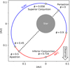 |
Fig. 1. LS 5039 system as determined by Casares et al. (2005) with an orbital period of Porb = 3.9 d and an eccentricity of e = 0.35, assuming a stellar mass Mstar = 23 M⊙ and a pulsar mass Mpulsar = 1.4 M⊙. Periastron, apastron, and the conjunctions are indicated. Matching the choices in Aharonian et al. (2006), the orbit is divided into two parts: INFC, ranging from 0.45 < ϕ < 0.9, and SUPC, for 0.9 < ϕ < 1 and 0 < ϕ < 0.45. We point out that, throughout the paper, the acronyms SUPC and INFC refer to the specified parts of the orbit, whereas the terms superior and inferior conjunction denote specific points on the orbit. |
To simulate the interacting fluids of the stellar wind and the pulsar wind, we numerically solved the equations of RHD, using a reference frame that co-rotates with the average angular velocity of the system, Ω = 2π/Porb (see Huber et al. 2021, for more details). The dynamical equations were solved using the CRONOS code (Kissmann et al. 2018). The simulation was performed on a Cartesian grid with dimensions [ − 1.25, 1.25]×[−0.5, 1.5]×[−0.5, 0.5] AU3, which is homogeneously subdivided into 640 × 512 × 256 spatial cells. The binary orbits in the x − y plane, with its centre of mass coinciding with the coordinate origin.
For the simulation of the wind interaction (presented in Sect. 3.1), we adopted a stellar mass loss rate of Ṁs = 2 × 10⁻⁸ M⊙ yr−1 and a terminal velocity of vs = 2000 km s−1 (Dubus et al. 2015). The speed of the pulsar wind was set to vp = 0.99 c, corresponding to a Lorentz factor of  . While this is smaller than conventional values,
  (see e.g., Khangulyan et al. 2012; Aharonian et al. 2012, and references therein), it is still high enough to capture the relevant relativistic effects (Bosch-Ramon et al. 2012). The pulsar mass loss rate
  was scaled with η = 0.1, yielding a corresponding pulsar spin-down luminosity Lsd = 7.55 × 1028 W. Both the stellar wind and the pulsar wind were continuously injected within a spherical region with radius rinj = 0.08 a around each object, which were initially placed in a vacuum. To account for the eccentricity of the orbit, the locations of the injection volumes were updated accordingly after every step of the simulation.
The simulation was performed for approximately 1.6 orbits. The first 0.6 orbits were used to initialise the simulation, allowing the slower stellar wind to populate the computational domain. The stellar wind reaches the farthest corner of the simulation box after tcrossing ≈ 0.45Porb ≈ 1.75 d. The subsequent full orbit was used for the scientific analysis.
For the evolution of the accelerated electron-positron pairs, we solved a Fokker-Planck-type transport equation simultaneously with the fluid interaction using an extension to the CRONOS code (Huber et al. 2021). For the particles, we used 50 logarithmic bins in energy covering the range γ ∈ [200, 4 × 10⁸]. At the acceleration sites – identified by a strongly compressive fluid flow ∇μuμ < −10 c/AU, where uμ is the fluid four-velocity – we injected two particle populations into the simulation: a power-law component, corresponding to accelerated, non-thermal pairs, and a Maxwellian component, corresponding to isotropised pairs from the pulsar wind (see also Dubus et al. 2015). For the sake of brevity, we refer to these particles only as electrons for the rest of this work. The non-thermal electrons were injected with a spectral index s = 1.5 and an acceleration efficiency ξacc = 2, which determines the maximum energy,  , reached by balancing the shock acceleration and synchrotron losses with the magnetic field strength B′. We assumed a fraction
  of the local internal fluid energy and a fraction
  of the number of available electrons from the pulsar wind to be injected as a non-thermal component. The remaining electrons were injected as a Maxwellian component. Since the pulsar-wind Lorentz factor used in our simulation might be higher in reality, the density of the pair plasma would be overestimated in our simulation. To account for this, we decreased the number of available electrons considered in the injection by a factor of ζρ = 5.5 × 10⁻⁴.
In our simulation, we did not evolve the magnetic field explicitly, which makes assumptions on its spatial dependence necessary. Therefore, we conducted the simulations under the assumption that the magnetic field energy density in the fluid frame is proportional to the internal energy density of the fluid,  (in analogy to Barkov & Bosch-Ramon 2018) with ζb = 0.5. This approximation is similar to the one used in Dubus et al. (2015) at the location of the shocks. Although the evolution of the magnetic field might differ in the shocked downstream flow, this approximation was expected to yield good values at the shocks, which are the most relevant for the particle injection. For the stellar companion, we assumed a luminosity L⋆ = 1.8 × 10⁵ L⊙, temperature T⋆ = 39 000 K, and resulting radius R⋆ = 9.3 R⊙ (Casares et al. 2005).
3. Results
3.1. Fluid structure
In Fig. 2 we show the resulting fluid mass density for different orbital phases. An extended WCR is formed from the PW-SW interaction, creating a bow-like shock (hereafter the bow shock) on the pulsar side. The overall shape of the WCR is highly asymmetric and bends in the direction opposite to the orbital motion due to the Coriolis force acting on the rotating system. The additional force leads to a termination of the pulsar wind on the far side of the system, forming another shock at the Coriolis turnover (hereafter the Coriolis shock).
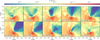 |
Fig. 2. Fluid mass density in the orbital plane for different orbital phases, indicated by the inset annotations. An extended WCR is formed due to the interaction of the pulsar (blue) and stellar (orange) wind. The reference frame is co-rotating with the anticlockwise orbital motion. The labels INFC and SUPC correspond to respective parts of the orbit as defined in Fig. 1. The boundaries between the inner and middle regions and between the middle and far regions (further discussed in the text) are indicated by the dashed and dotted lines, respectively. |
In the downstream region of the Coriolis shock, the shocked pulsar wind is turbulently mixed with shocked stellar-wind material, slowing the flow due to the increased mass load (see also Fig. A.1). Many secondary shocks are formed in the turbulent motion of the fluid, which can re-energise already cooled particles accelerated at other shocks (Bosch-Ramon et al. 2012). In the wings of the WCR, the pulsar wind shocked at the bow is re-accelerated towards its initial Lorentz factor (see also Bogovalov et al. 2008) until it reaches the turbulently mixed fluid behind the Coriolis shock, creating an additional shock (hereafter the reflected shock, in analogy to Dubus et al. 2015) that extends diagonally into the region behind the pulsar (clearly visible at ϕ ≃ 0.3 in Figs. 2 and A.2). Features visible in our simulation are in qualitative agreement with previous works (see e.g., Bosch-Ramon et al. 2015), validating our fluid model.
While the Coriolis shock location is in agreement with previous works at periastron, its distance from the pulsar becomes too large and leaves the computational domain around apastron. This suggests that the simulation box does not capture enough of the leading edge of the WCR (in front of the pulsar with respect to the anticlockwise orbital motion), which therefore cannot sweep up enough dense stellar-wind material to build up the required pressure to terminate the pulsar wind.
The structure of the WCR is strongly influenced by turbulence that develops at the contact discontinuity in the WCR. In addition to the Kelvin-Helmholtz (KH) instabilities triggered by the large velocity shear, the arising turbulence is further increased by Rayleigh-Taylor (RT) and Richtmeyer-Meshkov (RM) instabilities (Bosch-Ramon et al. 2012). This dominantly occurs at the leading edge of the WCR because there the high-density, shocked stellar wind is pressed against the low-density, shocked pulsar wind by the Coriolis force (see also Bosch-Ramon et al. 2012). We found that the formation of the Coriolis shock is influenced by the arising turbulence (see e.g., ϕ ≃ 0.8 in Fig. 2), which can cause orbit-to-orbit variations in the WCR structure.
The development of KH instabilities is strongly suppressed for highly relativistic flows (see e.g., Perucho et al. 2004; Bodo et al. 2004). Fluctuations can therefore only efficiently grow in the vicinity of the wind standoff, where the shocked pulsar wind is sufficiently slow with a speed of ∼c/3 before being re-accelerated. The timescale for advection out of this region therefore critically determines the largest modes that can be excited in the system since the growth rate for KH instabilities, ΓKH ∝ λ−1, decreases with larger wavelengths (see Bodo et al. 2004; Lamberts et al. 2013). The maximum wavelength of fluctuations that can be excited in the presented system is of the order of λmax ∼ 0.1 AU (assuming a region extension of ∼0.3 AU and an average advection velocity of ∼0.5 c).
The pulsar-wind Lorentz factor used in our simulation is lower than the typically assumed values ∼104 − 106 due to numerical limitations. A higher pulsar-wind Lorentz factor would yield a faster re-acceleration (Bosch-Ramon et al. 2012) when the shocked flow is expanding in the wings and might therefore reduce the advection timescale and shift the maximum wavelength of growing fluctuations to smaller values. However, Bogovalov et al. (2008) found that even in the ultra-relativistic limit, the shocked pulsar-wind flow remains slow near the head of the bow shock up to scales of the orbital separation for our choice of η. This is mainly a consequence of the bow-like geometry of the WCR, which causes the upstream incident angle with the shock normal to be small over a wide part of the head of the bow shock, leading to a strongly slowed downstream flow. Furthermore, the flow cannot expand rapidly there, keeping the re-acceleration at a moderate level. The re-acceleration only becomes more important farther out, where the opening angles of the pulsar-wind shock and the contact discontinuity approach their asymptotic values. The extent of the unstable region hence cannot go below the scales of the order of the orbital separation regardless of the pulsar-wind Lorentz factor, thus only slightly changing the estimates from above. Even in the ultra-relativistic limit, KH instabilities are therefore still expected to grow and the overall structure of the WCR should not change significantly.
For our setup, we found in numerical tests (simulating the decay of shear flows as described by Ryu & Goodman 1994) that damping by numerical viscosity Γdamp ∝ λ−3 dominates over the KH growth rate (estimated from Bodo et al. 2004) for short-wavelength fluctuations with λ ≲ 10−2 AU. The chosen resolution, therefore, allows the growth of fluctuations in the range 10−2 AU ≲ λ ≲ 10−1 AU (as seen in Fig. 2), where the larger wavelengths will have the biggest impact on the WCR. This also implies that future higher-resolution simulations will extend the range of turbulence to smaller spatial scales for which the driving by KH instabilities becomes more efficient because ΓKH ∝ λ−1.
In our simulation, we did not consider any feedback of the accelerated particles onto the fluid dynamics. Because the non-thermal electrons contribute a significant fraction of the overall energy density, their cooling will result in a decrease in the fluid’s pressure that supports the WCR. Consequently, when taking such feedback into account, the WCR will be less extended and might thus be more susceptible to thin-shell instabilities (as pointed out by Dubus et al. 2015), as it was seen in the case of colliding-wind binaries by Reitberger et al. (2017). The consideration of such effects is left for future work.
3.2. Particle distribution
Since the timescale for the particle populations to reach a quasi-steady state (by reaching the limits of the computational domain and/or by cooling) is orders of magnitudes smaller than the orbital timescale, we did not perform a particle transport simulation for the full time span of the fluid simulation. Instead, to reduce the computational effort, we restarted a particle transport simulation on previously obtained fluid solutions for the ten chosen orbital phases shown in Fig. 2. We performed these simulations for t = 1.11 h, allowing the injected electrons to populate the system.
To simulate the energetic evolution of the electrons, we employed the semi-Lagrangian scheme described in Huber et al. (2021). For this, we used the same time step as for the preceding hydrodynamic step, which is mainly determined by the speed of the un-shocked pulsar wind and the spatial resolution, yielding typical values of Δt ∼ 0.8 s. Due to the semi-Lagrangian nature of the scheme, an additional reduction of the time step depending on the energy resolution is not required to maintain stability.
In Figs. 3 and 4 we present the resulting electron distributions for different orbital phases at two energies, which are dominantly populated by Maxwellian and power-law electrons, respectively. The relevant shock structures are imprinted in the electron distributions. This is especially visible for particles at higher energies, which are quickly cooled through synchrotron and inverse Compton losses. Due to increased losses, they remain much more confined to their injection sites. Lower-energetic electrons, in comparison, dominantly lose energy via adiabatic losses and are therefore cooled on longer timescales, populating a much larger spatial domain. In addition to the bow and Coriolis shocks, the reflected shock and the countless secondary shocks in the turbulent downstream region behind the pulsar are also manifestly visible. In our simulation, radiative losses are highest at the wind standoff, which limits the maximum electron energy reached in the acceleration as well as the length scales over which non-thermal electrons are cooled afterwards. At the Coriolis shock, both the magnetic field and the stellar-radiation field are weaker in comparison and the highest particle energies of the simulation are reached (see Fig. 5).
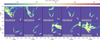 |
Fig. 3. Differential particle number density for electrons with γ = 3.11 × 10³ in analogy to Fig. 2. The arrows indicate the projected direction to an observer at Earth. For clarity, we show only five orders of magnitude below the highest value – the blue regions correspond to those with lower values. |
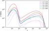 |
Fig. 5. Spectral energy distribution of electrons integrated over the computational domain for different orbital phases (colour-coded solid lines). For ϕ = 0.393, the contributions of the inner (dashed line), middle (dash-dotted), and outer regions (dotted) are shown as examples. |
In Fig. 5 we show the spectral energy distribution of the electrons integrated over the computational volume. The contributions of the Maxwellian and the power-law electrons can be easily distinguished as they dominate the energy range below and above γ ∼ 2 × 10⁴, respectively. It is apparent that not only the normalisation but also the shape of the spectrum are a function of the orbital phase, considering the location of the peak in the Maxwellian electrons, the break in the power-law tail, and the maximum energies reached. Furthermore, it shows that a higher electron density is reached after periastron, which is not intuitive at first glance.
This becomes more apparent in Fig. 6, where we show the temporal evolution of the electron distribution integrated over the computational volume at selected energies. Apparently, the number of electrons in the computational volume lags behind the orbit, that is, the minimum amount of electrons is reached after apastron and the maximum after periastron.
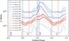 |
Fig. 6. Temporal evolution of the spectral energy distribution of energetic electrons integrated over the computational domain for selected energies (colour-coded). For a better visualisation, we show the same data for two orbits. |
This delay is caused by the inertia of the fluid. The WCR needs a certain amount of time to build up or dissipate its pressure, which critically determines the amount of electrons accelerated at the shocks. This phenomenon can only be seen in approaches that treat the particle transport together with the underlying fluid. The varying size of the shocks counteracts parts of this effect by shrinking and enlarging the acceleration sites at periastron and apastron, respectively; however, this is not dominant in our simulation. The power injected at the shocks reaches its maximum at ϕ ≃ 0.2 in our simulation, suggesting an expected peak in the integrated electron distribution with the same delay.
We find, however, that this delay is energy-dependent. While the number of higher-energetic electrons peaks as expected around ϕ ≃ 0.2, the number of lower-energetic ones peaks earlier, at ϕ ≃ 0.1 (see Fig. 6). This behaviour originates in the turbulent flow behind the pulsar formed earlier around the periastron passage, which leads to a pileup of electrons at lower energies, in turn yielding an earlier peak in their evolution. This effect is not relevant for electrons at higher energies since they are cooled much faster through radiative losses. Consequently, these particles are more confined to the shocks, preventing a pileup and leaving their number density more directly affected by the acceleration process.
We treated both the spectral slope and the acceleration efficiency as free model parameters since the specifics for particle acceleration in gamma-ray binaries have not yet been firmly identified. In this phenomenological approach, we treated all acceleration sites the same, which might not be the case in reality. For example, in the case of diffusive shock acceleration, both the spectral index and the acceleration timescale depend on the shock’s compression ratio, magnetic obliquity, and up- and downstream fluid velocities (see e.g., Keshet & Waxman 2005; Takamoto & Kirk 2015). In future efforts, the current model can be extended to investigate different acceleration mechanisms.
3.3. Emission
In this section, we present the simulation results for the non-thermal emission spectrum and light curves of LS 5039. They were produced in a post-processing step, using the previously obtained particle distributions (see Sect. 3.2) and fluid solutions (see Sect. 3.1). We, therefore, generated direct predictions on the initially spelt-out set of model parameters (see Sect. 2).
For the computation of the inverse Compton emission, we treated the stellar photon field as monochromatic, whereas a full blackbody spectrum was considered for the γγ-absorption. In both cases, the source was treated as an extended sphere. We computed the emission for two different system inclinations, i = 30° and i = 60°.
In our approach, it is no longer straightforward to separate the emission produced through particles accelerated at the different shocks, like it was possible in previous works (e.g., Dubus et al. 2015), since the downstream flows are turbulently mixed; this had previously been neglected. To obtain a basic understanding of the location dependence of the emission, we subdivided the computational volume into three regions (hereafter the inner, middle, and far regions), the boundaries of which are located at distances of 1.2 d and 3.5 d from the binary’s centre of mass, where d is the time-dependent orbital distance (see Fig. 2). In Sect. 3.3.1 we present the predicted emission spectra followed by a more detailed discussion for individual energy bands in Sects. 3.3.2–3.3.4. A projection map of the emission is discussed in Sect. 3.5.
3.3.1. Emission spectrum
In Fig. 7 we show the resulting spectral energy distributions of photons emitted for two different inclinations of the system, integrated over different orbital phases: To facilitate a comparison to observations, the orbit has been split into two parts, INFC and SUPC, as defined in Aharonian et al. (2006) (see Fig. 1). To compute the average spectra, we integrated the simulated ones using piece-wise linear interpolations in time.
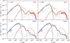 |
Fig. 7. Spectral energy distribution of the emission predicted by our model for LS 5039 for different parts of the orbit and inclinations of the system. Different radiative processes are colour-coded: synchrotron (green lines), inverse Compton (orange), inverse Compton attenuated by γγ-absorption (red), and total (black). The contributions to the total emission from the inner (dashed lines), middle (dashed-dotted), and far regions (dotted) are shown separately (for a description of the regions, see the main text). The model predictions are shown together with observations in soft X-rays (Takahashi et al. 2009) as well as LE (Collmar & Zhang 2014), HE (Hadasch et al. 2012), and VHE (Aharonian et al. 2006) gamma-rays. Results are shown for different parts of the orbit as defined in Fig. 1, with INFC on the top and SUPC on the bottom, and for different inclinations i of the orbital plane, with i = 30° on the left and i = 60° on the right. |
The spectral features of the particle population leave clear imprints in the emission spectrum. Ranging from X-rays up to LE gamma-rays, the spectrum is dominated by synchrotron emission generated by electrons at the power-law tail of the spectrum, which are dominantly produced in the inner region. The same population of electrons is responsible for the inverse Compton scattering of stellar UV photons into the VHE gamma-ray regime, although the relative contributions of the individual regions to the VHE emission is not constant but varies along the orbit. The emission in the HE gamma-ray regime is also produced through the inverse Compton process, however, by the lower-energetic Maxwellian electrons in the inner region of the system.
3.3.2. X-rays and LE gamma-rays
For the chosen set of parameters, the synchrotron emission predicted by our model is able to explain the observed X-ray to LE gamma-ray emission spectrum (see Fig. 7). This was not possible in previous studies (Dubus et al. 2015; Molina & Bosch-Ramon 2020). Synchrotron emission dominates up to ∼10 MeV, with a spectral cutoff approximately constant over the orbit. The electrons emitting at the LE cutoff are at the highest end of the power-law tail, accelerated at the apex of the bow shock. These particles are strongly confined to shocks and, thus, rely on our injection model and the conditions directly at the shock. This means that the synchrotron cutoff directly depends on two factors: the maximum electron energy (see Sect. 2) and the maximum photon energy produced through the synchrotron process. Both quantities depend only on the magnetic field, however, counteracting each other and leading to a constant synchrotron cutoff.
While the model predictions closely resemble the X-ray and LE gamma-ray observations at INFC, the X-ray flux is over-predicted at SUPC. This deviation is also manifest in the X-ray light curve (see the first row of Fig. 8). Instead of the observed correlation with VHE gamma-rays, the predicted X-ray light curve is correlated with the HE gamma-ray flux. This is caused by the still simplistic magnetic field description employed in our model: Since the magnetic field strength scales directly with the fluid pressure, its maximum at the bow shock is reached shortly after periastron. In addition, electron acceleration is also increased in this part of the orbit. The combined effects lead to a modulation of the synchrotron emissivity that dominates over that introduced by relativistic boosting, which was argued to be the dominant source of variability in this band (Dubus et al. 2015). These problems, therefore, highlight the necessity for a more sophisticated magnetic field description in future modelling.
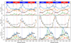 |
Fig. 8. Emission light curves predicted by our model for LS 5039 for different energy bands and inclinations of the system. The contributions from the inner (dashed orange lines), middle (dashed-dotted green lines), and far regions (dotted red lines) together with their sum (solid blue lines) are shown (for a description of the regions, see the main text). For better visualisation, we show the same data for two orbits. The results are shown for different energy bands together with observations in individual rows (from top to bottom): soft X-rays (1−10 keV; Takahashi et al. 2009), HE gamma-rays (0.2−3 GeV; Hadasch et al. 2012), and VHE (>1 TeV; Aharonian et al. 2006) gamma-rays. In the left column, results are shown for an inclination i = 30° of the orbital plane, while in the right column the results for an inclination i = 60° are presented. In addition to the orbital phases described in the main text, we show three more light curve points at ϕ ∼ 0.55, 0.65, and 0.85. The error bars indicate the variability introduced by turbulence (see Sect. 3.4). |
We also investigated the effects of different magnetic field models, such as a passively advected magnetic energy density wB injected together with the pulsar wind and/or a magnetic field aligned with the fluid bulk motion. The injected magnetic energy density is scaled with the injected kinetic energy density as  , where σ is the pulsar wind magnetisation fraction, yielding the magnetic field in the laboratory frame
  . We found little difference in the resulting emission spectra when using these alternative models for similar magnetic field strengths; they still yielded disagreement for the predicted X-ray light curve.
For larger inclination angles (see the right column in Fig. 8), relativistic boosting becomes more important. This decreases the X-ray flux at superior conjunction while increasing it at inferior conjunction, which better resembles the features of the observed light curve.
3.3.3. HE gamma-rays
While the overall spectral shape and the flux of the predicted HE emission are in good agreement with observations at SUPC, the predictions prove to be problematic at INFC (see Fig. 7). There, the predicted HE flux drops by approximately one order of magnitude and the spectrum is shifted towards lower energies, leaving the fluxes under-predicted. These changes in the flux are mainly caused by the anisotropic inverse Compton scattering cross-section, which grows with the scattering angle. At phases around superior conjunction, stellar photons have to be scattered by a larger angle to reach the observer as compared to inferior conjunction. Consequently, the highest and lowest inverse Compton fluxes relate to these phases, respectively. The anisotropic scattering further causes the shift in energy, yielding higher scattered photon energies for larger scattering angles. Both effects can also be seen by comparing the different inclination angles (e.g., see Fig. 7).
An additional modulation is generated by the changing stellar seed radiation field density induced by the varying distance of the bow shock apex to the star, with the maximum and minimum stellar photon densities at periastron and apastron, respectively. Due to the geometry of the LS 5039 orbit, the periastron passage occurs very close to superior conjunction, leading this modulation to be added to the former one.
The underestimation of the HE gamma-ray flux at INFC suggests a missing component in our broadband emission model, which could arise from the magnetospheric emission of the pulsar as suggested by, for example, Takata et al. (2014). This process can naturally account for the phase-independent spectral cutoff of the HE emission at energies of a few GeV. To accommodate this emission within our modelling, one would have to find a new set of parameters for the Maxwellian electron distribution to avoid an overestimation of the flux at SUPC.
The discrepancy is also apparent in the predicted HE light curves (see the second row in Fig. 8), which show a phase-independent underestimation with respect to the observations. Disregarding the constant under-prediction, the light curve for an inclination of i = 30° is in good agreement with observations. For the higher inclination angle, the inverse Compton anisotropy leads to a steep rise in emission at superior conjunction, while it further reduces the flux at phases around apastron and inferior conjunction.
Inverse Compton emission by relativistic Maxwellian pairs in the cold pulsar wind might yield another contribution in this energy band. The current model does not take this contribution into account explicitly since the required ultra-relativistic pulsar wind Lorentz factor,  , cannot be captured by our numerical methods. The produced spectra, however, strongly resemble the ones produced by the Maxwellian electrons injected at the shocks in our model (see Takata et al. 2014). Due to this degeneracy, the emission produced by the Maxwellian electrons effectively capture this contribution in our modelling.
3.3.4. VHE gamma-rays
In contrast to the HE gamma-ray emission, the flux at VHE is heavily attenuated by γγ-absorption, introducing an additional line-of-sight-dependent modulation. The observed spectral features and the temporal characteristics are well recovered by our model, with a high-energy cutoff in excellent agreement with observations and a pronounced anti-correlation with the HE gamma-ray emission, as shown in Fig. 7 and the third row in Fig. 8, respectively.
Due to γγ-absorption, the VHE-flux, especially from the inner region, is strongly reduced for all phases (see Fig. 7). At INFC, the larger inclination of i = 60° is favourable because the absorption is weakened by smaller scattering angles as compared to i = 30°. Here, the dominant part of the emission is produced in the middle region with strong relativistic boosting, leading to a hard spectrum, as seen in observations. The increased contribution of this region around inferior conjunction can also be seen more directly in Fig. 9, where we illustrate the relative contribution to the gamma-ray flux as a function of distance from the binary’s centre of mass.
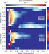 |
Fig. 9. Relative contribution to the radiation emitted at a given orbital phase from spherical shells around the system’s centre of mass (with a thickness of 0.05 AU) at two different energies. For clarity, we only present the results for a system inclination of i = 60°; the resulting maps qualitatively agree with those for an inclination i = 30°. We terminate the analysis at r = 1.5 AU, where the farthest edge of the computational volume is reached. Relevant orbital phases are annotated (see also Fig. 1). |
In the 100 GeV to 1 TeV range, where the γγ-absorption is most pronounced, the flux is underpredicted with respect to observations for SUPC. At phases around superior conjunction, the emission produced in both the inner and middle regions is almost completely attenuated by absorption, as shown in Fig. 9, leaving the radiation to be dominantly produced in the far region of the system. The predicted fluxes, however, are too small to reproduce observations around periastron and superior conjunction (see the third row in Fig. 8) in our simulations. We found that the region that dominates the flux reaching the observer in the energy range most affected by γγ-absorption around superior conjunction is extended over a large volume behind the pulsar (see Fig. 9). In particular, it extends to the edges of the computational volume, suggesting that a fraction of the emission is lost by particles leaving the domain. A larger computational domain is required to address this issue, which goes beyond the scope of available computational resources.
For a system inclination of i = 60°, we find a sharp peak in the predicted VHE light curve at ϕ ≃ 0.55 (see the third row in Fig. 8). At this phase, the observer’s line-of-sight is aligned with the leading edge of the shocked pulsar wind flow, yielding a drastically increased photon flux due to relativistic boosting (which can also be seen at the bottom of Fig. 9) that is incompatible with observations. The trailing edge of the WCR is crossed by the observer between ϕ ≃ 0.8 and ϕ ≃ 0.9 in our simulation, showing no peaked emission.
3.4. Turbulence-induced variability
To assess the impact of short-term variability introduced by turbulence on the system’s radiative output, we evolved the particle distributions presented in Sect. 3.2 for a longer time and recomputed the emission. After the initial convergence time of t0 = 1.11 h, we investigated the particle distributions at tn = t0 + n ⋅ Δt, with Δt = 0.14 h and n = 0, 1, 2, 3, 4. This time increment, Δt, is sufficiently longer than the growth timescale of KH instabilities (see also Sect. 3.1) for the different solutions to be uncorrelated. For each orbital phase we computed the average and the standard deviation from the five obtained emission solutions; we show the results in Fig. 8.
We found that turbulence introduces variability depending on the orbital phase and photon energy, with typical variability levels of several per cent, though reaching ∼17% for the HE flux around superior conjunction and ∼12% for the VHE flux around inferior conjunction. Most of the variability is apparent in the inner and middle regions, which is expected since these regions are most directly affected by instabilities formed at the contact discontinuity. Although turbulence introduces visible flux fluctuations, they are still considerably smaller than orbital variations and thus do not dominate the resulting light curves.
Lastly, we found that the pulsar-wind shock structure is influenced by turbulence that develops at the stellar-wind shock on longer timescales (see Sect. 3.1). This has an effect on the variability on orbital timescales and is expected to introduce orbit-to-orbit variations, which will be studied in the future when more computational resources become available.
3.5. Emission map
For a better visualisation of the emission produced in LS 5039, we show a composite false-colour emission map in Fig. 10 as it would be seen with a perfect angular resolution at Earth. The imprint of the fluid structure is clearly visible, exhibiting the bow shock and the turbulent downstream region behind the pulsar around periastron. At ϕ ≃ 0.1 the star eclipses parts of the emission region, occluding a circular region on the map.
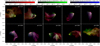 |
Fig. 10. Projection of the predicted emission from LS 5039 for different orbital phases with an orbital plane inclination of i = 60°. The differential energy flux is shown for distinct energy bands as indicated by the colour bars. For better visualisation, the upper limits of the colour bars have been set two orders of magnitude lower than the maximum HE gamma-ray flux. |
4. Summary and discussion
In this work we present the application of a novel numerical model for gamma-ray binaries (Huber et al. 2021) to the LS 5039 system. We specifically chose this system for its broad observational coverage, known orbital parameters, and comparison to previous modelling efforts.
Our simulations of the wind interaction in this system show an extended asymmetric WCR that is bent by the orbital motion, exhibiting a strong bow-like pulsar-wind shock and a Coriolis shock behind the pulsar. With our approach, it is, for the first time, possible to consistently account for the complex dynamic shock structure in the particle transport model. In addition to the bow and Coriolis shocks, this also includes the reflection shock (formed where the downstream plasma of bow and Coriolis shocks collide) and the secondary shocks (which arise in the turbulent downstream medium of the Coriolis shock). The resulting structures are in agreement with those observed in previous simulations (see Bosch-Ramon et al. 2015), although the Coriolis shock is not formed in the numerical domain at phases around inferior conjunction. This is caused by the computational domain being too small to capture enough of the leading edge of the WCR to reach the required pressure to terminate the pulsar wind at the respective phases. In simulations with a larger computational domain, the Coriolis shock is expected to reappear – possibly so close to the pulsar that it would be within the extents of the current computational domain.
We find that the extrema of the fluid’s internal energy do coincide with orbital extrema, as assumed by previous studies (see e.g., Dubus et al. 2015; Zabalza et al. 2013; Takata et al. 2014). This affects the resulting particle distributions since most of the models, including the presented one, scale the amount and energetics of accelerated electrons with the available internal fluid energy. This results in a delay of the electron density extrema of Δϕ ≃ 0.1−0.2 in our model, depending on their energy. This delay also translates to the production of radiation; however, it is compensated for in part by the onset of relativistic de-boosting at superior conjunction (shortly after periastron) in the case of LS 5039.
Our model reproduces the main spectral features of the observed emission from LS 5039, ranging from soft X-rays to VHE gamma-rays, further substantiating a wind-driven interpretation of gamma-ray binaries. In contrast to previous studies (e.g., Dubus et al. 2015), our simulation predicts that the synchrotron emission connects the X-ray emission to the LE gamma-ray emission. We attribute this result to the different WCR geometry, which affects relativistic boosting, and to our improved treatment of the star as an extended photon source, leading to increased γγ-absorption. Similar to previous studies (e.g., Dubus et al. 2015; Molina & Bosch-Ramon 2020), we find that a hard spectral index of s = 1.5 is required for the electron acceleration to describe the observations. The predicted spectra underestimate the flux in the HE gamma-ray band, presumably lacking a contribution by the magnetospheric emission of the pulsar (Takata et al. 2014).
While the inner region (<1.2 orbital separations d from the system’s centre of mass) provides the bulk of the emission from X-rays to HE gamma-rays, the middle and far regions (1.2−3.5 d and > 3.5 d, respectively) are especially relevant for the emission in the VHE band mainly due to relativistic beaming and γγ-absorption. Our conclusions contrast the assessment by Molina & Bosch-Ramon (2020), who found the far region to be the dominant emitter for all energies and orbital phases. This directly relates to different assumptions regarding the injection of non-thermal electrons into the system. While we assume the same fraction of the fluid’s internal energy density to be converted to non-thermal electrons at all shocks, Molina & Bosch-Ramon (2020) assume that a significantly larger fraction of the pulsar’s spin-down luminosity is converted at the Coriolis shock than at the bow shock; this is not the case in our simulations.
Our model predicts significant orbital modulation in all energy bands, mainly originating via the anisotropic inverse Compton process, relativistic boosting, and the changing properties of the WCR. While the predicted HE to VHE gamma-ray light curves agree with observations, the simulations fail to reproduce the observed orbital X-ray and LE gamma-ray modulation. Instead of the observed correlation with VHE gamma-rays, a correlation with the HE band is predicted. We attribute this to the rather simplistic magnetic field model (i.e. scaling the magnetic energy density with the fluid pressure), which varies strongly across the orbit and is responsible for the dominant modulation in the synchrotron emissivity. Such a model has been employed in previous studies that use a semi-analytical description for the emitting particles (e.g., Barkov & Bosch-Ramon 2018), but it seems to be increasingly incompatible with our more detailed particle transport model, highlighting the need for a more sophisticated approach. This could be realised, for example, via an extension of the presented model to relativistic magnetohydrodynamics. With this, it will be possible to take the impact of the non-negligible magnetic field on the fluid dynamics into account, yielding a more realistic picture of the magnetic field strength and direction, and in turn enabling more realistic injection models and the consideration of anisotropic synchrotron emission.
At INFC, the middle region produces the dominant contribution to the VHE gamma-ray spectrum due to relativistic boosting, allowing a hard spectral index to be maintained. We note that the Coriolis shock is not present in the simulation for most of the corresponding phases, as mentioned previously. Its presence in larger simulations is expected to reduce the size of the bow shock wings, where this relativistically boosted emission originates, which might lead to a softening of the spectrum.
At superior conjunction, a significant part of the VHE gamma-ray emission is produced by electrons in the far region of the system due to the weakened impact of γγ-absorption. However, emitting particles are lost at the boundaries of the simulation. We suspect this to be the main reason for the underestimation of the SUPC flux in the 100 GeV to 1 TeV range and the underestimation of the VHE light curve around periastron to superior conjunction. These issues as well as the missing Coriolis shock at some orbital phases can be addressed by employing a larger computational volume.
We found that turbulence formed in the wind interaction introduces sub-orbital variability in the system’s radiative output on the levels of several per cent on average, reaching up to ∼20 per cent for certain orbital phases and photon energies. The introduced variations in the flux, however, are still considerably smaller than those on orbital timescales. On longer timescales, turbulence is expected to introduce orbit-to-orbit variations, which cannot be studied from the single simulated orbit. This shows the need for further investigations on larger timescales and a larger spatial domain.
Both investigated inclinations of the orbital plane yield fluxes that are more or less consistent with observations depending on the considered energy band. The HE gamma-ray light curve slightly favours a lower inclination of i = 30°, due to the amplitude of the modulation, whereas the VHE gamma-ray spectrum prefers the larger inclination of i = 60°, due to the hard spectral index. The latter inclination is also favourable because it makes the X-ray light curve more consistent with observations by overcoming parts of the strong internal modulation of the synchrotron emissivity due to the increased relativistic boosting.
Although a larger inclination proves to be favourable due to the later decrease of the VHE flux after superior conjunction, the predicted VHE light curve at i = 60° shows a peak that is incompatible with observations shortly after apastron, arising from relativistic boosting when the leading edge of the shocked pulsar wind flow is crossed by the observer’s line-of-sight (see also Dubus et al. 2015). We note again that the amplitude of the VHE peak might be overestimated in the presented work because of the missing Coriolis shock at the phases of the peak.
Since the employed simulations take the naturally arising asymmetric shape of the WCR into account, the trailing edge is considerably wider as compared to the leading edge when the observer’s line-of-sight is crossed, smearing out the effects of relativistic boosting. This prevents the formation of the second peak in the VHE light curve around ϕ ∼ 0.85 that has been seen for higher inclinations in previous works that employ a more simplified prescription of the WCR (Dubus et al. 2015). Such a second peak is not visible in related observations.
In this study, we showed the feasibility of a combined fluid and particle-transport simulation for predicting the radiative output of gamma-ray binaries. Future extensions of this model, as discussed, are expected to lead to a better representation of the observations of LS 5039 and will be applied to other well-observed gamma-ray binaries.
Acknowledgments
The computational results presented in this paper have been achieved (in parts) using the research infrastructure of the Institute for Astro- and Particle Physics at the University of Innsbruck, the LEO HPC infrastructure of the University of Innsbruck, the MACH2 Interuniversity Shared Memory Supercomputer and PRACE resources. We acknowledge PRACE for awarding us access to Joliot-Curie at GENCI@CEA, France. This research made use of Cronos (Kissmann et al. 2018); GNU Scientific Library (GSL) (Galassi et al. 2018); matplotlib, a Python library for publication quality graphics (Hunter 2007); and NumPy (Van Der Walt et al. 2011). We thank the anonymous referee for the thoughtful comments and suggestions that allowed us to improve our manuscript.
References
- Abdo, A. A., Ackermann, M., Ajello, M., et al. 2009, ApJ, 706, L56 [NASA ADS] [CrossRef] [Google Scholar]
- Aharonian, F., Akhperjanian, A. G., Aye, K. M., et al. 2005, Science, 309, 746 [NASA ADS] [CrossRef] [PubMed] [Google Scholar]
- Aharonian, F., Akhperjanian, A. G., Bazer-Bachi, A. R., et al. 2006, A&A, 460, 743 [NASA ADS] [CrossRef] [EDP Sciences] [Google Scholar]
- Aharonian, F. A., Bogovalov, S. V., & Khangulyan, D. 2012, Nature, 482, 507 [NASA ADS] [CrossRef] [PubMed] [Google Scholar]
- Barkov, M. V., & Bosch-Ramon, V. 2018, MNRAS, 479, 1320 [Google Scholar]
- Bodo, G., Mignone, A., & Rosner, R. 2004, Phys. Rev. E, 70, 036304 [NASA ADS] [CrossRef] [Google Scholar]
- Bogovalov, S. V., Khangulyan, D. V., Koldoba, A. V., Ustyugova, G. V., & Aharonian, F. A. 2008, MNRAS, 387, 63 [Google Scholar]
- Bosch-Ramon, V., & Khangulyan, D. 2009, Int. J. Mod. Phys. D, 18, 347 [Google Scholar]
- Bosch-Ramon, V., & Barkov, M. V. 2011, A&A, 535, A20 [NASA ADS] [CrossRef] [EDP Sciences] [Google Scholar]
- Bosch-Ramon, V., Khangulyan, D., & Aharonian, F. A. 2008, A&A, 489, L21 [NASA ADS] [CrossRef] [EDP Sciences] [Google Scholar]
- Bosch-Ramon, V., Barkov, M. V., Khangulyan, D., & Perucho, M. 2012, A&A, 544, A59 [NASA ADS] [CrossRef] [EDP Sciences] [Google Scholar]
- Bosch-Ramon, V., Barkov, M. V., & Perucho, M. 2015, A&A, 577, A89 [NASA ADS] [CrossRef] [EDP Sciences] [Google Scholar]
- Casares, J., Ribó, M., Ribas, I., et al. 2005, MNRAS, 364, 899 [Google Scholar]
- Cerutti, B., Malzac, J., Dubus, G., & Henri, G. 2010, A&A, 519, A81 [NASA ADS] [CrossRef] [EDP Sciences] [Google Scholar]
- Collmar, W., & Zhang, S. 2014, A&A, 565, A38 [NASA ADS] [CrossRef] [EDP Sciences] [Google Scholar]
- Dubus, G. 2006, A&A, 451, 9 [NASA ADS] [CrossRef] [EDP Sciences] [Google Scholar]
- Dubus, G. 2013, A&ARv, 21, 64 [Google Scholar]
- Dubus, G., Cerutti, B., & Henri, G. 2008, A&A, 477, 691 [NASA ADS] [CrossRef] [EDP Sciences] [Google Scholar]
- Dubus, G., Cerutti, B., & Henri, G. 2010, A&A, 516, A18 [NASA ADS] [CrossRef] [EDP Sciences] [Google Scholar]
- Dubus, G., Lamberts, A., & Fromang, S. 2015, A&A, 581, A27 [NASA ADS] [CrossRef] [EDP Sciences] [Google Scholar]
- Galassi, M., Davies, J., Theiler, J., et al. 2018, GNU Scientific Library Reference Manual (Network Theory Ltd) [Google Scholar]
- Hadasch, D., Torres, D. F., Tanaka, T., et al. 2012, ApJ, 749, 54 [Google Scholar]
- Huber, D., Kissmann, R., Reimer, A., & Reimer, O. 2021, A&A, 646, A91 [NASA ADS] [CrossRef] [EDP Sciences] [Google Scholar]
- Hunter, J. D. 2007, Comput. Sci. Eng., 9, 90 [NASA ADS] [CrossRef] [Google Scholar]
- Keshet, U., & Waxman, E. 2005, Phys. Rev. Lett., 94, 111102 [NASA ADS] [CrossRef] [Google Scholar]
- Khangulyan, D., Aharonian, F. A., Bogovalov, S. V., & Ribó, M. 2012, ApJ, 752, L17 [NASA ADS] [CrossRef] [Google Scholar]
- Kissmann, R., Kleimann, J., Krebl, B., & Wiengarten, T. 2018, ApJS, 236, 53 [Google Scholar]
- Lamberts, A., Fromang, S., Dubus, G., & Teyssier, R. 2013, A&A, 560, A79 [NASA ADS] [CrossRef] [EDP Sciences] [Google Scholar]
- Maraschi, L., & Treves, A. 1981, MNRAS, 194, 1P [Google Scholar]
- Mirabel, I. F. 2006, Science, 312, 1759 [Google Scholar]
- Molina, E., & Bosch-Ramon, V. 2020, A&A, 641, A84 [CrossRef] [EDP Sciences] [Google Scholar]
- Paredes, J. M., & Bordas, P. 2019, ArXiv e-prints [arXiv:1901.03624] [Google Scholar]
- Perucho, M., Martí, J. M., & Hanasz, M. 2004, A&A, 427, 431 [NASA ADS] [CrossRef] [EDP Sciences] [Google Scholar]
- Reitberger, K., Kissmann, R., Reimer, A., & Reimer, O. 2017, ApJ, 847, 40 [Google Scholar]
- Romero, G. E., Okazaki, A. T., Orellana, M., & Owocki, S. P. 2007, A&A, 474, 15 [NASA ADS] [CrossRef] [EDP Sciences] [Google Scholar]
- Ryu, D., & Goodman, J. 1994, ApJ, 422, 269 [NASA ADS] [CrossRef] [Google Scholar]
- Takahashi, T., Kishishita, T., Uchiyama, Y., et al. 2009, ApJ, 697, 592 [Google Scholar]
- Takamoto, M., & Kirk, J. G. 2015, ApJ, 809, 29 [NASA ADS] [CrossRef] [Google Scholar]
- Takata, J., Leung, G. C. K., Tam, P. H. T., et al. 2014, ApJ, 790, 18 [Google Scholar]
- Van Der Walt, S., Colbert, S. C., & Varoquaux, G. 2011, Comput. Sci. Eng., 13, 22 [Google Scholar]
- Zabalza, V., Bosch-Ramon, V., Aharonian, F., & Khangulyan, D. 2013, A&A, 551, A17 [NASA ADS] [CrossRef] [EDP Sciences] [Google Scholar]
Appendix A: Supplementary material
In this section we provide additional visualisation for the fluid quantities that have been omitted in the main text. In Figs. A.1–A.3 we show the fluid’s four-velocity, its thermal energy density, and the magnetic field strength in the fluid frame, respectively.
All Figures
|
Fig. 1. LS 5039 system as determined by Casares et al. (2005) with an orbital period of Porb = 3.9 d and an eccentricity of e = 0.35, assuming a stellar mass Mstar = 23 M⊙ and a pulsar mass Mpulsar = 1.4 M⊙. Periastron, apastron, and the conjunctions are indicated. Matching the choices in Aharonian et al. (2006), the orbit is divided into two parts: INFC, ranging from 0.45 < ϕ < 0.9, and SUPC, for 0.9 < ϕ < 1 and 0 < ϕ < 0.45. We point out that, throughout the paper, the acronyms SUPC and INFC refer to the specified parts of the orbit, whereas the terms superior and inferior conjunction denote specific points on the orbit. |
| In the text | |
|
Fig. 2. Fluid mass density in the orbital plane for different orbital phases, indicated by the inset annotations. An extended WCR is formed due to the interaction of the pulsar (blue) and stellar (orange) wind. The reference frame is co-rotating with the anticlockwise orbital motion. The labels INFC and SUPC correspond to respective parts of the orbit as defined in Fig. 1. The boundaries between the inner and middle regions and between the middle and far regions (further discussed in the text) are indicated by the dashed and dotted lines, respectively. |
| In the text | |
|
Fig. 3. Differential particle number density for electrons with γ = 3.11 × 10³ in analogy to Fig. 2. The arrows indicate the projected direction to an observer at Earth. For clarity, we show only five orders of magnitude below the highest value – the blue regions correspond to those with lower values. |
| In the text | |
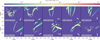 |
Fig. 4. Same as Fig. 3, but for γ = 1.05 × 10⁷. |
| In the text | |
|
Fig. 5. Spectral energy distribution of electrons integrated over the computational domain for different orbital phases (colour-coded solid lines). For ϕ = 0.393, the contributions of the inner (dashed line), middle (dash-dotted), and outer regions (dotted) are shown as examples. |
| In the text | |
|
Fig. 6. Temporal evolution of the spectral energy distribution of energetic electrons integrated over the computational domain for selected energies (colour-coded). For a better visualisation, we show the same data for two orbits. |
| In the text | |
|
Fig. 7. Spectral energy distribution of the emission predicted by our model for LS 5039 for different parts of the orbit and inclinations of the system. Different radiative processes are colour-coded: synchrotron (green lines), inverse Compton (orange), inverse Compton attenuated by γγ-absorption (red), and total (black). The contributions to the total emission from the inner (dashed lines), middle (dashed-dotted), and far regions (dotted) are shown separately (for a description of the regions, see the main text). The model predictions are shown together with observations in soft X-rays (Takahashi et al. 2009) as well as LE (Collmar & Zhang 2014), HE (Hadasch et al. 2012), and VHE (Aharonian et al. 2006) gamma-rays. Results are shown for different parts of the orbit as defined in Fig. 1, with INFC on the top and SUPC on the bottom, and for different inclinations i of the orbital plane, with i = 30° on the left and i = 60° on the right. |
| In the text | |
|
Fig. 8. Emission light curves predicted by our model for LS 5039 for different energy bands and inclinations of the system. The contributions from the inner (dashed orange lines), middle (dashed-dotted green lines), and far regions (dotted red lines) together with their sum (solid blue lines) are shown (for a description of the regions, see the main text). For better visualisation, we show the same data for two orbits. The results are shown for different energy bands together with observations in individual rows (from top to bottom): soft X-rays (1−10 keV; Takahashi et al. 2009), HE gamma-rays (0.2−3 GeV; Hadasch et al. 2012), and VHE (>1 TeV; Aharonian et al. 2006) gamma-rays. In the left column, results are shown for an inclination i = 30° of the orbital plane, while in the right column the results for an inclination i = 60° are presented. In addition to the orbital phases described in the main text, we show three more light curve points at ϕ ∼ 0.55, 0.65, and 0.85. The error bars indicate the variability introduced by turbulence (see Sect. 3.4). |
| In the text | |
|
Fig. 9. Relative contribution to the radiation emitted at a given orbital phase from spherical shells around the system’s centre of mass (with a thickness of 0.05 AU) at two different energies. For clarity, we only present the results for a system inclination of i = 60°; the resulting maps qualitatively agree with those for an inclination i = 30°. We terminate the analysis at r = 1.5 AU, where the farthest edge of the computational volume is reached. Relevant orbital phases are annotated (see also Fig. 1). |
| In the text | |
|
Fig. 10. Projection of the predicted emission from LS 5039 for different orbital phases with an orbital plane inclination of i = 60°. The differential energy flux is shown for distinct energy bands as indicated by the colour bars. For better visualisation, the upper limits of the colour bars have been set two orders of magnitude lower than the maximum HE gamma-ray flux. |
| In the text | |
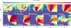 |
Fig. A.1. Fluid four-speed in analogy to Fig. 2. |
| In the text | |
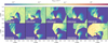 |
Fig. A.2. Fluid thermal energy in analogy to Fig. 2. |
| In the text | |
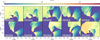 |
Fig. A.3. Magnetic field in the fluid frame in analogy to Fig. 2. |
| In the text | |
Current usage metrics show cumulative count of Article Views (full-text article views including HTML views, PDF and ePub downloads, according to the available data) and Abstracts Views on Vision4Press platform.
Data correspond to usage on the plateform after 2015. The current usage metrics is available 48-96 hours after online publication and is updated daily on week days.
Initial download of the metrics may take a while.